8.4 Camera setup for building the table of real-world actuator effects. . . 181. 8.5 Robot ...... World Community Grid [URL - World Community Grid] is a similar, but.
Pavel Petrovic Incremental Evolutionary Methods for Automatic Programming of Robot Controllers
Thesis for the degree philosophiae doctor Trondheim, November 2007 Norwegian University of Science and Technology Faculty of Information Technology, Mathematics and Electrical Engineering Department of Computer and Information Science
Innovation and Creativity
NTNU Norwegian University of Science and Technology Thesis for the degree philosophiae doctor Faculty of Information Technology, Mathematics and Electrical Engineering Department of Computer and Information Science © Pavel Petrovic ISBN 978-82-471-5031-3 (printed version) ISBN 978-82-471-5045-0 (electronic version) ISSN 1503-8181 Doctoral theses at NTNU, 2007:228 Printed by NTNU-trykk
Abstract The aim of the main work in the thesis is to investigate Incremental Evolution methods for designing a suitable behavior arbitration mechanism for behavior-based (BB) robot controllers for autonomous mobile robots performing tasks of higher complexity. The challenge of designing effective controllers for autonomous mobile robots has been intensely studied for few decades. Control Theory studies the fundamental control principles of robotic systems. However, the technological progress allows, and the needs of advanced manufacturing, service, entertainment, educational, and mission tasks require features beyond the scope of the standard functionality and basic control. Artificial Intelligence has traditionally looked upon the problem of designing robotics systems from the high-level and top-down perspective: given a working robotic device, how can it be equipped with an intelligent controller. Later approaches advocated for better robustness, modifiability, and control due to a bottom-up layered incremental controller and robot building (Behavior-Based Robotics, BBR). Still, the complexity of programming such system often requires manual work of engineers. Automatic methods might lead to systems that perform task on demand without the need of expert robot programmer. In addition, a robot programmer cannot predict all the possible situations in the robotic applications. Automatic programming methods may provide flexibility and adaptability of the robotic products with respect to the task performed. One possible approach to automatic design of robot controllers is Evolutionary Robotics (ER). Most of the experiments performed in the field of ER have achieved successful learning of target task, while the tasks were of limited complexity. This work is a marriage of incremental idea from the BBR and automatic programming of controllers using ER. Incremental Evolution allows automatic programming of robots for more complex tasks by providing a gentle and easy-to understand support by expertknowledge — division of the target task into sub-tasks. We analyze different types of incrementality, devise new controller architecture, implement an original simulator compatible with hardware, and test it with various incremental evolution tasks for real robots. We build up our experimental field through studies of experimental and educational robotics systems, evolutionary design, distributed computation that provides the required processing power, and robotics applications. University research is tightly coupled with education. Combining the robotics research with educational applications is both a useful consequence as well as a way of satisfying the necessary condition of the need of underlying application domain where the research work can both reflect and base itself.
Preface When the robots will start going skiing of their own will, the age of robots will have come. My first meeting with programmable robots occurred as an instructor in the summer camp for talented young children in the early 90s where we were programming a simple LEGO-built scanner and greenhouse using a dialect of Logo running on Macintosh Classic. Later on, professor Sam Thangiah introduced me to real mobile robots (B12 from the Real World Interfaces) that we programmed in assembly and C as the assignments for his Machine Learning course at Slippery Rock in Pennsylvania. He also introduced me to the capabilities and applications of Evolutionary Computation. Arriving to NTNU threw me into more unavoidable hands-on LEGO experience and hacking, where I was lucky to remain part of the increasing interest in robotics and robotics contests at all age levels. The studies in the field of artificial intelligence give me strong arguments to believe that there is a good chance for the robots being able to start sharing a common environment with us while being at our service soon. The realization is the job for the industry. In academia, we ought to overcome the scientific and technological barriers, develop algorithms, and methods. It is now the most interesting time when such technologies get born, and this work is a tiny contribution into that area. During my graduate studies, I happened to get involved in several different projects cooperating with different people and groups, while keeping work on my own lonely thesis thread at the same time. In this paper, I would like to share with you all of that, keeping the main focus on my own original ideas, while including all the cooperative work, which relates to it and joins into one common theme Evolutionary Robotics.
Acknowledgments First of all, I would like to express my appreciations to the institute and the faculty for providing me with a creative, inspiring, and friendly working environment for an extensive period of time. Several colleagues contributed to the outcome. The most valuable feedback and care was always received from my adviser, professor Keith Downing. Thanks to his strong principles and dedication, and due to the scientifically appreciating environment created by the group and division leader professor Agnar Aamodt, the laboratory for sub-symbolic artificial intelligence existed at our department throughout the whole duration of this work, and served as a wonderful place to exchange the ideas among us, the students. I thank to Zoran Constantinescu F¨ ul¨op for productive cooperation on the distributed computation tools and projects, and for sharing a lot of valuable work and time. A special thanks belongs to the technical group of the department. Without their support, running the experiments in the student laboratories would be impossible. I am very grateful to professor Henrik Hautop Lund from Maersk institute in Odense and his colleagues, who allowed me to spend one semester with them and who contributed with a very useful feedback. ˇ I am thankful to the members of Robotika.SK, namely Duˇsan Durina, Richard Balogh, Andrej L´ uˇcny, and Jozef Omelka, who provided a great robotics learning environment during my civil service year in Slovakia. I am committed to my parents and sister, who sought for my personal happiness especially during my visits at home, as well as for my comfort (a special thanks for all those warm hand-made wool pullovers). And finally, big hug to all the Norwegian, Greek, Spanish, Italian, French, Dutch, German, Finish, American, African, Portuguese, Danish, and even Czech and Slovak, and other girls I met during the years, they were a great inspiration, and it was all worth just that. :)
Disclaimer LEGO, LEGO Mindstorms, LEGO Mindstorms NXT, BlueTooth, SONY, Aibo, Khepera, and other trademarks appearing in the text are owned by the respective owners.
Contents 1 Introduction 11 1.1 Research Questions Addressed in the Thesis . . . . . . . . . . . . . . 15 2 Background 2.1 Introduction and Social Implications . . . . . . . . . . . . . . . . . . 2.2 Robotics and Artificial Intelligence . . . . . . . . . . . . . . . . . . . 2.3 Evolving Robotics . . . . . . . . . . . . . . . . . . . . . . . . . . . . . 2.4 Embodiment, Situatedness, Environment . . . . . . . . . . . . . . . . 2.5 Planning and Reactivity . . . . . . . . . . . . . . . . . . . . . . . . . 2.6 Navigation . . . . . . . . . . . . . . . . . . . . . . . . . . . . . . . . . 2.7 Sensors and Actuators . . . . . . . . . . . . . . . . . . . . . . . . . . 2.8 Vision . . . . . . . . . . . . . . . . . . . . . . . . . . . . . . . . . . . 2.9 Controller Architectures . . . . . . . . . . . . . . . . . . . . . . . . . 2.10 Finite-State Automata as Representation for Evolutionary Algorithms 2.11 Robot Programming Formalisms . . . . . . . . . . . . . . . . . . . . . 2.12 Behavior-Based Robotics . . . . . . . . . . . . . . . . . . . . . . . . . 2.12.1 Representing Behaviors in a Controller . . . . . . . . . . . . . 2.12.2 Arbitration Mechanisms . . . . . . . . . . . . . . . . . . . . . 2.12.3 Team Robotics with Behavior-Based Architectures . . . . . . . 2.13 Evolutionary Robotics . . . . . . . . . . . . . . . . . . . . . . . . . . 2.13.1 Evolvable Tasks . . . . . . . . . . . . . . . . . . . . . . . . . . 2.13.2 Fitness Space . . . . . . . . . . . . . . . . . . . . . . . . . . . 2.13.3 Co-Evolution . . . . . . . . . . . . . . . . . . . . . . . . . . . 2.13.4 Evolving the Robot Morphology . . . . . . . . . . . . . . . . . 2.13.5 Evolving Behavior Arbitration . . . . . . . . . . . . . . . . . . 2.13.6 Incremental Evolution . . . . . . . . . . . . . . . . . . . . . . 2.14 Simulation and Real Robotic Experiments . . . . . . . . . . . . . . . 2.15 Chapter Summary . . . . . . . . . . . . . . . . . . . . . . . . . . . .
17 17 18 19 20 25 26 28 29 30 32 34 35 36 36 38 39 40 42 42 43 43 45 48 51
3 Research Goals and Hypotheses 3.1 Introduction . . . . . . . . . . . . . 3.2 Evolving Robotics . . . . . . . . . . 3.3 Robotic Task Complexity . . . . . 3.4 Arbitration Mechanisms . . . . . . 3.5 Embedded Evolution . . . . . . . . 3.6 Evolutionary Adaptive Mechanisms
53 53 55 56 57 58 58
. . . . . .
. . . . . .
. . . . . .
. . . . . .
. . . . . .
. . . . . .
. . . . . .
. . . . . .
. . . . . .
. . . . . .
. . . . . .
. . . . . .
. . . . . .
. . . . . .
. . . . . .
. . . . . .
. . . . . .
. . . . . .
. . . . . .
2
Contents 3.7 Aspects of Incremental Evolution . . . . . . . . . . 3.7.1 Sequential vs. Structural . . . . . . . . . . . 3.7.2 Population Transition . . . . . . . . . . . . 3.7.3 Emergent vs. Engineered Steps . . . . . . . 3.7.4 Automatic Division into Incremental Stages 3.8 Controller Architecture Goals . . . . . . . . . . . . 3.9 Simulation . . . . . . . . . . . . . . . . . . . . . . . 3.10 Chapter Summary . . . . . . . . . . . . . . . . . .
. . . . . . . .
. . . . . . . .
. . . . . . . .
. . . . . . . .
. . . . . . . .
. . . . . . . .
59 61 63 66 66 67 70 71
. . . . . . . . . . . . . .
. . . . . . . . . . . . . .
73 73 76 77 77 78 78 79 79 83 84 85 85 86 89
5 Supporting Studies 5.1 Role of Robotics in Education . . . . . . . . . . . . . . . . . . . . . 5.1.1 Robotics in Elementary and Secondary Schools . . . . . . . 5.1.2 Guidelines for Educators: Curriculum, Skills and Philosophy 5.1.3 Teaching-Learning Materials . . . . . . . . . . . . . . . . . . 5.1.4 Robotics Contests . . . . . . . . . . . . . . . . . . . . . . . . 5.2 Creative Educational Platforms . . . . . . . . . . . . . . . . . . . . 5.3 Ten Educational Projects . . . . . . . . . . . . . . . . . . . . . . . . 5.4 Evolve with Imagine – Educational Evolutionary Environment . . . 5.4.1 Recombination . . . . . . . . . . . . . . . . . . . . . . . . . 5.4.2 Mutation . . . . . . . . . . . . . . . . . . . . . . . . . . . . 5.4.3 Selection and Other Parameters and Features . . . . . . . . 5.5 Evolution of Shape and Form . . . . . . . . . . . . . . . . . . . . . 5.5.1 Representational Aspects of Evolving Form and Shape . . . 5.5.2 Experimental Setup . . . . . . . . . . . . . . . . . . . . . . . 5.5.3 Results . . . . . . . . . . . . . . . . . . . . . . . . . . . . . . 5.6 Chapter Summary . . . . . . . . . . . . . . . . . . . . . . . . . . .
. . . . . . . . . . . . . . . .
91 91 92 93 95 96 96 100 103 103 104 105 106 106 112 113 118
4 Supporting Technologies 4.1 RCX as a Research Hardware Platform . . . . . . . . . . . . 4.2 Distributed Computing . . . . . . . . . . . . . . . . . . . . . 4.3 Q2 ADP Z - Tool for Distributed Computation . . . . . . . . 4.3.1 Motivation . . . . . . . . . . . . . . . . . . . . . . . . 4.3.2 Features . . . . . . . . . . . . . . . . . . . . . . . . . 4.3.3 User Modes . . . . . . . . . . . . . . . . . . . . . . . 4.3.4 Inter-Platform Operability . . . . . . . . . . . . . . . 4.3.5 Architecture . . . . . . . . . . . . . . . . . . . . . . . 4.3.6 Utilizing the Q2 ADP Z for EC Experiments . . . . . 4.4 Evolutionary Computation and Distributed Computing . . . 4.5 Distributed Evolutionary Algorithm . . . . . . . . . . . . . . 4.5.1 Utilizing the Cluster Computing for EC Experiments 4.5.2 Universal Solution . . . . . . . . . . . . . . . . . . . 4.6 Chapter Summary . . . . . . . . . . . . . . . . . . . . . . .
. . . . . . . . . . . . . . . . . . . . . .
. . . . . . . . . . . . . . . . . . . . . .
. . . . . . . . . . . . . . . . . . . . . .
. . . . . . . .
6 Comparison of FSA and GP-tree Representations 119 6.1 Introduction and Aims . . . . . . . . . . . . . . . . . . . . . . . . . . 119 6.1.1 Representations . . . . . . . . . . . . . . . . . . . . . . . . . . 120
CONTENTS 6.1.2 Search Space . . . . . . 6.1.3 Sensitive Operators . . . 6.2 Experimental Setup . . . . . . . 6.2.1 Experiment “bit collect” 6.2.2 Experiment “(abcd)n ” . 6.2.3 Experiment “switch” . . 6.2.4 Experiment “find target” 6.2.5 Experiment “dock” . . . 6.3 Results . . . . . . . . . . . . . . 6.4 Chapter Summary . . . . . . .
3 . . . . . . . . . .
. . . . . . . . . .
. . . . . . . . . .
. . . . . . . . . .
. . . . . . . . . .
. . . . . . . . . .
. . . . . . . . . .
. . . . . . . . . .
. . . . . . . . . .
. . . . . . . . . .
. . . . . . . . . .
. . . . . . . . . .
. . . . . . . . . .
. . . . . . . . . .
. . . . . . . . . .
. . . . . . . . . .
. . . . . . . . . .
. . . . . . . . . .
. . . . . . . . . .
. . . . . . . . . .
. . . . . . . . . .
123 124 125 125 126 127 127 130 130 156
7 Design and Implementation Considerations 7.1 Simulation Framework . . . . . . . . . . . . . . . . . . 7.1.1 Lazy Simulation Method . . . . . . . . . . . . . 7.1.2 Simulation Time and Multithreaded Scheduling 7.1.3 Functional Requirements for the Simulator . . . 7.1.4 Detailed Simulation Procedure . . . . . . . . . . 7.2 Controller Architecture . . . . . . . . . . . . . . . . . . 7.3 Evolutionary Algorithm . . . . . . . . . . . . . . . . . 7.3.1 Representation . . . . . . . . . . . . . . . . . . 7.3.2 Operators . . . . . . . . . . . . . . . . . . . . . 7.3.3 Scaling . . . . . . . . . . . . . . . . . . . . . . . 7.3.4 Checkpoints . . . . . . . . . . . . . . . . . . . . 7.4 Chapter Summary . . . . . . . . . . . . . . . . . . . .
. . . . . . . . . . . .
. . . . . . . . . . . .
. . . . . . . . . . . .
. . . . . . . . . . . .
. . . . . . . . . . . .
. . . . . . . . . . . .
. . . . . . . . . . . .
. . . . . . . . . . . .
157 157 157 160 162 165 166 168 170 170 173 175 176
8 Experimental Work 8.1 Simple Adaptive Autonomous Robot . . . . . . . 8.2 Incremental Evolution . . . . . . . . . . . . . . . 8.2.1 Embedded Incremental Evolution . . . . . 8.2.2 Structured Task for Incremental Evolution 8.3 Results . . . . . . . . . . . . . . . . . . . . . . . . 8.3.1 Embedded Incremental Evolution . . . . . 8.3.2 Cargo Transporting Task . . . . . . . . . . 8.4 Chapter Summary . . . . . . . . . . . . . . . . .
. . . . . . . .
. . . . . . . .
. . . . . . . .
. . . . . . . .
. . . . . . . .
177 177 179 179 180 187 187 190 201
9 Discussion and Conclusions 9.1 Discussion . . . . . . . . . . . . . . . . . . . . . . 9.1.1 Extensibility of the Controller . . . . . . . 9.1.2 Evolution Modeled as Phenotypic Process 9.1.3 From FSA to Recurrent NN Architectures 9.1.4 Lessons Learned about Simulating Robotic 9.1.5 Symbolic and Sub-Symbolic Viewpoints . . 9.2 Main Contributions of the Thesis . . . . . . . . . 9.3 Conclusions . . . . . . . . . . . . . . . . . . . . . 9.3.1 On Educational Robotics . . . . . . . . . .
. . . . . . . . . . . . . . . . . . . . . . . . . . . . . . . . System Time . . . . . . . . . . . . . . . . . . . . . . . . . . . . . . . .
. . . . . . . . .
. . . . . . . . .
. . . . . . . . .
203 203 203 204 206 207 207 210 212 217
. . . . . . . .
. . . . . . . .
. . . . . . . .
. . . . . . . .
. . . . . . . .
. . . . . . . .
4 Appendix A – List of EI Parameters
Contents 220
Appendix B – Example of Specification of Environment for the Simulator 225 Appendix C – Example of Specification of Evolutionary Run
233
Bibliography
251
Index
265
List of Figures 2.1 Emergence robotics experiment, implementation with RCX robots. 2.2 Importance of the relation between robot morphology and controller, program fragment. . . . . . . . . . . . . . . . . . . . . . . . . . . . 2.3 Importance of the relation between robot morphology and controller, phases of ball following. . . . . . . . . . . . . . . . . . . . . . . . . 2.4 Importance of the relation between robot morphology and controller, changing the angular range. . . . . . . . . . . . . . . . . . . . . . . 2.5 Influence of the robot morphology on performance, drawing of a sensor installation. . . . . . . . . . . . . . . . . . . . . . . . . . . . 2.6 A motor schema for 2D environment with 4 obstacles . . . . . . . . 2.7 Stimulus-response diagram and functional notation of behaviors. . . 2.8 Behavior arbitration general framework. . . . . . . . . . . . . . . . 2.9 An example of a controller built using the Subsumption Architecture of Brooks. . . . . . . . . . . . . . . . . . . . . . . . . . . . . . . . . 2.10 Robotics simulation by means of emulating robot controller. . . . . 3.1 An example of scenario consisting of sequential incremental steps: window-cleaning robot. . . . . . . . . . . . . . . . . . . . . . . . . . 3.2 An example of scenario of incremental steps following a tree-structure: basketball playing robot. . . . . . . . . . . . . . . . . . . . . . . . . 3.3 An example of scenario of incremental steps that form a directed acyclic graph: berry-collecting robot. . . . . . . . . . . . . . . . . . 3.4 Population mixing in an incremental scenario. . . . . . . . . . . . . 3.5 Extensibility of the controller. . . . . . . . . . . . . . . . . . . . . . 3.6 Single behavior module with its arbitrating post-office finite-state machines. . . . . . . . . . . . . . . . . . . . . . . . . . . . . . . . . 4.1 4.2 4.3 4.4 4.5 4.6 4.7 4.8 4.9 4.10
Reliable post-office protocol for PC-RCX communication. . Infra-red / Bluetooth conversion module for RCX. . . . . . Q2 ADP Z: A simple library-type project file. . . . . . . . . Q2 ADP Z: Simple executable-type project file. . . . . . . . Q2 ADP Z: Slave status message. . . . . . . . . . . . . . . Q2 ADP Z architecture. . . . . . . . . . . . . . . . . . . . . Q2 ADP Z communication layers. . . . . . . . . . . . . . . List of slaves – status information provided by master. . . Overall architecture of the distributed evolutionary system. Utilization of two versions of distributed algorithm. . . . .
. . . . . . . . . .
. . . . . . . . . .
. . . . . . . . . .
. . . . . . . . . .
. . . . . . . . . .
. 22 . 23 . 24 . 24 . . . .
25 27 36 37
. 38 . 50 . 62 . 62 . 63 . 65 . 68 . 69 . . . . . . . . . .
74 75 79 80 80 81 82 83 85 86
6
List of Figures 5.1 Students from secondary school in Trondheim preparing their robot for the RoboCup Junior contest in Bremen, June 2006. . . . . . . . . 94 5.2 Viewing the remotely-accessible robotics laboratory in a web-browser. 98 5.3 Interfacing the robots in the remotely-accessible laboratory from C. . 99 5.4 Solution to the example 1. . . . . . . . . . . . . . . . . . . . . . . . . 101 5.5 Solution to the example 2. . . . . . . . . . . . . . . . . . . . . . . . . 101 5.6 View from the top-mounted camera, the same image recognized by the image recognition plug-in for Imagine, drawing a convex hull. . . 102 5.7 Voronoi representation genotype and phenotype. . . . . . . . . . . . . 107 5.8 Holes representation with various geometric shapes creates more natural shapes using less shapes than rectangular-holes representation.108 5.9 Standard LEGO bricks used in layer layouts. . . . . . . . . . . . . . . 110 5.10 Shapes used in the topological optimum design experiment. . . . . . . 112 5.11 Comparison of the performance of the roulette-wheel selection and steady-state GA. . . . . . . . . . . . . . . . . . . . . . . . . . . . . . 113 5.12 Best individual fitness with standard deviations (random 3D models 20x20x5) for layer 4. . . . . . . . . . . . . . . . . . . . . . . . . . . . 114 5.13 Example runs of 16x16 TOD shape with different genotype representations. . . . . . . . . . . . . . . . . . . . . . . . . . . . . . . . . . . . 115 5.14 Best fitness (average of 20 runs) for the four different representations, 8x8 shape. . . . . . . . . . . . . . . . . . . . . . . . . . . . . . . . . . 115 5.15 Best fitness (average of 20 runs) for the four different representations, 16x16 shape. . . . . . . . . . . . . . . . . . . . . . . . . . . . . . . . . 116 5.16 Best fitness (average of 20 runs) for the four different representations, 32x32 shape. . . . . . . . . . . . . . . . . . . . . . . . . . . . . . . . . 116 5.17 The first two layers evolved with steady-state GA. . . . . . . . . . . . 117 5.18 Shapes with evolved brick layouts, from [Na, 2002]. . . . . . . . . . . 117 5.19 Comparison of the performance of the improved GA that has features of indirect representations (repetitive brick placements), [Na, 2002]. . 117 6.1 6.2 6.3 6.4 6.5 6.6 6.7 6.8 6.9 6.10
Illustration of GP-tree representation. . . . . . . . . . . . . . . . . . Illustration of FSA representation. . . . . . . . . . . . . . . . . . . . Environments for the find target task. . . . . . . . . . . . . . . . . . Viewing the progress of simulation in a web browser using a viewer implemented as Java applet. . . . . . . . . . . . . . . . . . . . . . . Average of the fitness of the best individuals in the find target task. Example trajectories of evolved individuals using the GP-tree and the FSA representations in find target task. . . . . . . . . . . . . . . . . Trajectories of the best individuals from all generations in find target task. . . . . . . . . . . . . . . . . . . . . . . . . . . . . . . . . . . . Trajectories of the best individuals from final generation in find target task, complex environment. . . . . . . . . . . . . . . . . . . . . . . Generalization of the evolved solutions when started from different starting locations in find target task, complex environment. . . . . . Performance of the FSA and GP-tree representations in find target task, environment ten around. . . . . . . . . . . . . . . . . . . . . .
. 121 . 122 . 128 . 129 . 131 . 133 . 133 . 134 . 134 . 135
LIST OF FIGURES
7
6.11 Trajectories of the best individuals from final generation in find target task, environment ten around. . . . . . . . . . . . . . . . . . . . . . 6.12 Generalization of the evolved solutions when started from different starting locations in find target task, ten around environment. . . . 6.13 Performance of the FSA and GP-tree representations on simple version of task bit collect. . . . . . . . . . . . . . . . . . . . . . . . . . 6.14 Performance of the FSA and GP-tree representations on more complex version of task bit collect. . . . . . . . . . . . . . . . . . . . . . 6.15 Performance of the FSA and GP-tree representations on task abcdn . 6.16 Average of the best fitness on a switch task with four symbols for both representations. . . . . . . . . . . . . . . . . . . . . . . . . . . 6.17 Average of the best fitness on a switch task with three symbols for both representations. . . . . . . . . . . . . . . . . . . . . . . . . . . 6.18 The best evolved FSA in the switch task with three symbols. . . . . 6.19 Average of the best fitness on a 4-symbol switch task, comparison of incremental and non-incremental runs. . . . . . . . . . . . . . . . . 6.20 Average of the best fitness on a 4-symbol switch task, comparison of fully incremental and non-incremental runs. . . . . . . . . . . . . . 6.21 Average of the best fitness on a 4-symbol switch task, comparison of fully incremental with freezing FSA and non-incremental runs. . . . 6.22 Average of the best fitness in the 4-symbol switch task, comparison of incremental runs with restricted terminal set and non-incremental runs. . . . . . . . . . . . . . . . . . . . . . . . . . . . . . . . . . . . 6.23 Performance of the GP-tree and FSA representations on simulated dock task. . . . . . . . . . . . . . . . . . . . . . . . . . . . . . . . . 6.24 A final evolved FSA in the dock task. . . . . . . . . . . . . . . . . . 6.25 Trajectories for the evolved individuals in typical runs, dock task. . 6.26 Trajectories for the evolved individuals in selected runs, dock task. . 6.27 Role of the crossover operator for the FSA representation in switch task with three symbols. . . . . . . . . . . . . . . . . . . . . . . . . 6.28 Comparison of two selection methods in experiment find target with environment experiment fence and the GP-tree representation. . . . 6.29 Comparison of two selection methods on experiment find target with environment ten around and the GP-tree representation. . . . . . . 6.30 Comparison of two selection methods, difficult version of the experiment bit collect and FSA representation. . . . . . . . . . . . . . . . 7.1 7.2 7.3 7.4 7.5 7.6 7.7 7.8 7.9
Simulated robot topology and features. . . . . . . . . . . . . . . . Simulation implementation method. . . . . . . . . . . . . . . . . . Loading station is specified using two active areas (top view). . . Unloading station is specified using three active areas. . . . . . . . Movement types for differential drive robot used in experiments. . Example controller architecture for a mouse acquiring cheese task. Controller architecture and genotype representation . . . . . . . . Example of crossover operator functionality. . . . . . . . . . . . . Crossover operator. . . . . . . . . . . . . . . . . . . . . . . . . . .
. . . . . . . . .
. 136 . 136 . 137 . 138 . 140 . 141 . 142 . 144 . 145 . 146 . 146
. 148 . . . .
149 152 153 154
. 154 . 155 . 155 . 156 . . . . . . . . .
159 161 164 164 167 167 169 171 175
8
List of Figures 8.1 8.2 8.3 8.4 8.5 8.6 8.7 8.8 8.9 8.10 8.11 8.12 8.13 8.14 8.15 8.16 8.17
Simple adaptive autonomous robot. . . . . . . . . . . . . . . . . . . Setup for the embedded evolutionary experiment. . . . . . . . . . . Environments for the embedded evolutionary experiment. . . . . . . Camera setup for building the table of real-world actuator effects. . Robot setup and environment for the cargo transporting task. . . . Experimental environments for 6 incremental evolutionary steps of creative incremental scenario. . . . . . . . . . . . . . . . . . . . . . FSA arbitrators for modules cargo-loader, avoidance, and explore. . Automatic detection of incremental step, analysis. . . . . . . . . . . Automatic detection of incremental step, complex environment. . . Embedded evolution task, complex environment and evolution of best fitness. . . . . . . . . . . . . . . . . . . . . . . . . . . . . . . . . . . Cargo transporting task, environment and real-robot setup. . . . . . Cargo transporting task, plot of the best fitness in steps of the creative incremental scenario. . . . . . . . . . . . . . . . . . . . . . . . . . . Cargo transporting task, finite-state machines evolved in each step of creative scenario. . . . . . . . . . . . . . . . . . . . . . . . . . . . . Cargo transporting task, plot of the best fitness in steps of the sequential scenario. . . . . . . . . . . . . . . . . . . . . . . . . . . . Contribution of mutation operators to evolutionary progress. . . . . Positive rate of mutation operators. . . . . . . . . . . . . . . . . . . Examples of evolved misbehavior in cargo transporting task. . . . .
. . . . .
178 180 180 181 182
. . . .
185 186 188 189
. 190 . 191 . 193 . 195 . . . .
197 198 199 200
9.1 A re-planning controller for a pick-and-place robot enabled with a camera and image recognition. . . . . . . . . . . . . . . . . . . . . . . 208 9.2 A prototype of LEGO pick-and place robot. . . . . . . . . . . . . . . 209
List of Tables 6.1 6.2 6.3 6.4 6.5
The number of binary trees of depth 1-10. . . . . . . . . . . . . . . . 124 A final evolved GP-tree and FSA for the environment experiment fence.132 A final evolved GP-tree and FSA for the environment ten around. . . 136 A final evolved GP-tree and FSA, task abcdn . . . . . . . . . . . . . . 139 The number of states in the evolved FSA and the number of states that are reachable in the switch task with three symbols. . . . . . . . 141 6.6 Evolved frozen individuals in the incremental steps 1–4, switch task with four symbols. . . . . . . . . . . . . . . . . . . . . . . . . . . . . 147 6.7 The best evolved GP-tree solution in the dock task without penalty. . 150 6.8 Selected evolved individuals with the best performance for the dock task. . . . . . . . . . . . . . . . . . . . . . . . . . . . . . . . . . . . . 151 8.1 Message interfaces for behavioral modules. . . . . . . . . . . . . . . . 184 8.2 Cargo transporting task, number of evaluations in steps of the creative scenario. . . . . . . . . . . . . . . . . . . . . . . . . . . . . . . . . . . 192 8.3 Cargo transporting task, number of evaluations in steps of the sequential scenario. . . . . . . . . . . . . . . . . . . . . . . . . . . . . . 196
10
List of Tables
Chapter 1 Introduction The job of a research worker is similar to the one of a concerting musician. The music itself controls every single movement of the musician in order to elude a beautiful harmony of sounds prescribed by the composer. Similarly, the nature controls every single movement of the researcher in order to unveil the secrets of its own harmony. In order to utilize ever advancing technological developments of materials, power supplies, computer technology, sensors, and actuators in the field of robotics, suitable controller architectures at a correspondingly advanced level need to be developed for these devices. Mobile robots could perform complicated tasks in unknown, non-deterministic, changing, noisy, and unpredictable environments, if methods for designing robot controllers could be developed. Successful completion of tasks will require the controllers to be adaptive and sometimes learning. Systematic research efforts to study possible methods for building such controllers are to be spent. Researchers and engineers have been designing and studying controllers for autonomous mobile robots since the 1950s (the famous Grey Walter’s Tortoise robot). Mainstream robotics systems are built upon the principles of the Control Theory. Artificial Intelligence traditionally approached the problem of designing robotics systems with the philosophical motivations of building machines that can think. The AI scientists acquired a working robotic device, and studied the problem of making it intelligent, their approach was clearly a top-down one. The naive attempt to design a complete system in this manner, i.e. to specify the whole system from the top to the bottom layers meets various constraints that make the approach at least difficult and not very efficient. The complexity of interactions of a mobile robotic system implies a structured (non-monolithic) controller architecture. Traditional AI approaches based on centralized-processing and Sense-Plan-Act cycle have difficulties dealing with simultaneous robot activities that have different priorities. Even if a purelyplanning controller would be successfully designed, its maintainability, modifiability, and performance would be compromised. Mobile agents must behave according to the outcome of several independent threads of reasoning. This requirement is implied by the highly parallel nature of events and processes in the real world. The controller architecture can meet this requirement if it is modular, and when the modules can act simultaneously in a coordinated cooperation.
12
Introduction
A new wave of AI robotics (as a part of Nouvelle AI) was started by the proponents of behavior-based systems. In these systems, the path to an intelligent being starts with building simple concrete functional creatures. Their behavior is controlled by a set of interacting modules. On the bottom side, these modules are as simple as direct reactive connections between sensors and actuators. On the top side, these modules might perform long-term reasoning inferences running in the background with a low priority. These ideas are reflected well in various behaviorbased and hybrid architectures, [Arkin, 1998]. Many studies focus on designing a framework, which possibly allows integration of higher-level functions and AI theories into BB architectures. We support this view, and we aim at studying particular aspects of the BB controller design. A BB controller consists of a set of relatively independent modules. Each of these modules is responsible for making sure that the robot will successfully perform certain behavior. The behavioral modules typically have control over the robot sensors and actuators, but their activation (arbitration) and combination of their outputs (command fusion) is a difficult challenge. One of the main challenges of the BB design is how the individual modules will be coordinated. This is referred to as action selection problem or behavior arbitration, see [Pirjanian, 1999] for an overview. Different action selection methods were studied before. On the side of arbitration, these include priority-based, state-based, and winner-take-all. On the side of command fusion, these include voting, superposition, fuzzy, and multiple-objective. The coordination mechanisms can be divided into state-based and continuous, where the state-based can work using either competitive or temporal sequencing principles. For tasks that involve learning, the action selection problem is deeply studied by research in Reinforcement Learning [Sutton and Barto, 1998], one of the most popular methods for automatic design of robot controllers. In these cases, the behavior arbitration or command fusion is a function to be learned based on the requirements of the task. In this thesis, we will work with BB systems without a predefined arbitration and command fusion mechanisms. On the contrary, these will be designed using Evolutionary Algorithm (EA), with the help of simulation of the robot performing in its environment. In particular, we will study how Incremental Evolution (IE) can be applied to the problem of the design of suitable action-selection mechanisms in BB controllers. Since the EAs proved to be successful in creating novel designs in various domains, our hypothesis and planned research contribution is to demonstrate how EAs can be used in this domain. Another strong motivation comes from the viewpoint of the field of Evolutionary Robotics (ER) itself. Approximately 15 years of research in the field brought successful robotic systems that can perform relatively simple low-level tasks, such as obstacle avoidance, wall following, or target tracking. The controllers are often based on arbitrarily-connected neural networks, [Beer and Gallagher, 1992]. Adaptive behaviors on a different level could possibly be achieved by approaches [Floreano and Urzelai, 2000] that evolve the neuron learning rules instead of the connection weights, which are changing dynamically during the task execution. Nevertheless, it appears that evolving more complex behaviors in a single evolutionary run is not
13 plausible due to a complex search space, and becomes impossible without additional guidance of the EA. Few researchers addressed tasks of a higher complexity. ER uses a bottom-up approach. The evolution typically starts at a complete bottom and has to discover the low-level control mechanisms. On one hand, this attributes to a very high flexibility in possibilities for the robot behavior that is formed. On the other hand, it severely limits the complexity of the task, which is to be performed. ER cannot reach beyond the low-level behaviors without a supporting framework, if it is to start at the bottom level. In the natural evolution, such framework was provided by the immense richness of the species, niches, and the environments, and the millions of years of evolutionary development. When artificial evolution is to serve as a design method, the framework must be replaced by other means. The evolved controller is not very likely to benefit from the structural properties of a BB-type controller, if such form will not be enforced. One way of self-guiding of an evolutionary algorithm is the use of co-evolution, [Hillis, 1990]. Co-evolution, however, applies best to that class of problems where two entities are competing for the same resource, or fight. In addition, it can be vulnerable to possible cyclic loops in the relation of strategy dominance in effect causing stagnation of the algorithm instead of progression. Another possible guidance, adopted also in this work, is dividing the target task into more simple incremental steps, [Harvey, 1995]. This strategy is more general; however, it requires a scenario of incremental evolutionary steps. How to devise such incremental steps, and how to setup such incremental EAs is the focus of this and future work. Designing a controller for a particular task for a mobile robot requires detailed knowledge of the robot hardware and software and an experienced engineer. We are seeking an alternative: automatic design of the controller. Our aim is to minimize the efforts and maximize the quality. The approach we promote in this thesis is to use ER with BB-type controller. We don’t put any particular constraints on how the individual behavioral modules are designed. Typically, engineers who designed the robot will provide the low-level control mechanisms, which will be well-tuned and efficient for the hardware the robot is equipped with. Alternately, low level behaviors can be learned or evolved. Given the set of low-level behaviors, and a particular task for the robot, the goal is to complete the design of the robot’s controller using EAs. The work lays at the intersection between BB Robotics and ER. By the means of EA, the design of the BB-controller adapts to the constraints of the specific task, robot, and environment. Higher complexity of the controller, when compared to other ER approaches, is achieved by the use of a BB-type controller with a set of predefined behaviors. We are dealing here with an adaptation at the level of the design process, where the resulting controller is adapted to the target task. Run-time adaptability of the robot itself can be achieved by learning in the individual behaviors, flexible arbitration or command-fusion mechanisms, and/or Embedded EC [Petroviˇc, 2001b], similar to Anytime Learning approach of [Grefenstette and Ramsey, 1992]. In this work, we aim at evolutionary design of behavior arbitration for a controller of a mobile robot performing a non-trivial task, where simple reactive controller
14
Introduction
would not be sufficient. The controller has a particular BB architecture, while the arbitration is based on a set of finite-state automata. The design is the output from an incremental evolutionary algorithm. During the work on the project, we were exposed to different projects, ideas, and environments. This brought us to the understanding that as advanced field as the field of robotics is, can hardly be studied without learning and taking into account a wider background — both from the AI-theoretical side that regards planning, optimization, evolutionary computation, machine learning, from the robot-design point of view that includes learning about sensors, actuators, building and lowlevel programming of robots, and from the educational point of view that includes bringing the world of robotics down to the schools at all levels — either to promote the computer and natural sciences among youngsters, or to provide modern motivating learning tools and technologies for students and researchers. This report, in addition to addressing the main research questions listed at the end of this chapter, reflects the work done and lessons learned in various aspects of this broader context. The thesis is organized into several chapters. The following chapter reviews the theoretical background and presents the approaches of the fields where this work attempts to make contributions. The third chapter analyzes and discusses the goals and hypotheses we set to reach and verify in more details. We describe the technologies we employed in the fourth chapter. We add to our arguments through a series of supporting studies, which we all describe in the fifth chapter including the results obtained. The representation formalism of the behavior arbitration mechanism, finite-state automata, are analyzed as a genotype representation and compared to Genetic Programming in a preliminary study in the sixth chapter. The following two chapters lay down a more detailed specification on how we prepared our experiments and studies on theoretical and more practical levels. The last chapter before the conclusions of the thesis describes and discusses the experiments we have performed as well as the results obtained.
1.1 Research Questions Addressed in the Thesis
1.1
15
Research Questions Addressed in the Thesis
The main research question of the thesis asks by which ways can Evolutionary Algorithms provide useful solutions to the problem of automatic design of controllers for mobile robots. Previously, EA have been successfully applied to designing robotic controllers with simple architectures based typically on Neural Networks. These approaches were applied to relatively simple navigational or operational tasks. As indicated by previous works, Incremental Evolution can increase evolvability when designing robot controllers for mobile robots. The design methods for robot controllers in the traditional Artificial Intelligence usually deal with symbolic reasoning mechanisms and make emphasis on planning, often involved in a centralized architecture. Alternately, the Nouvelle AI methods rely on incremental bottomup design of robot controllers that consist of independently executing behavioral modules with possibly conflicting intentions, desired actions, and effects. The particular concern of this work is whether and how the EA method could be successfully applied also to the controllers with architecture inspired by the Nouvelle AI, the behavior-based controllers. Is Incremental Evolution a useful method in this context, and what are the caveats of its application? The thesis will address the questions of which controller architectures suit the evolutionary behavioral approach particularly well and why. The thesis will work toward providing a complete functional solution and may include studies into related fields, building and implementing tools that may be required to reach satisfactory solution of automatic design of mobile robot controllers.
16
Introduction
Chapter 2 Background There is a noticeable difference between the national parks in Slovakia and Norway: In Slovakia, the visitors follow the well-prepared hiking trails and must not leave them. In Norway, the trails are often missing or very hard to find, while the tourists are free to choose any of their ways. In this chapter, we set on a path to explore the various topics related to robotics. The main aim of this work lies in incremental evolutionary robotics experiments. And we shall always keep in mind that it is there our path leads. It would be a somewhat unbalanced approach to jump right into a subject that is just a small flavor on top of something that is difficult to build, understand, implement, and grasp – successful robotic systems. In the spirit of bottom-up approaches, our journey started in the simplest form of robotics-experience encounters – robotics educational systems and efforts, which are explained in the fifth chapter together with supporting technologies we used for the experimental work in our thesis explained in the fourth chapter. This chapter touches upon the issues that are interesting and relevant for our perspective, although it is not meant to provide a comprehensive overview of the respective fields. In that spirit, we will gently cover the AI’s viewpoints on robotics and its challenges, arriving at Evolving Robotics, which is where our target lies all the long way ahead.
2.1
Introduction and Social Implications
Typical tasks, where robots can be useful, share common properties, such as hazardous or uncomfortable for humans, requiring heavy manipulation or tools, which are awkward to handle, or necessitating repetitive execution. Robots could be useful also in tasks, which can be carried out by humans, while performing with higher reliability, cheaper, faster, longer or even perpetually, or more efficiently. Some opponents of technological progress could claim that robots are taking the work from humans. And they are right, but we must comment on it that given the above conditions we do not find it a negative tendency, just the opposite. There are always many more things to be done than people available, and always many challenges to be worked on, and a long path for all of us ahead. Obviously, the enormous challenge
18
Background
will be finding and implementing a suitable economical and social model that can provide for distribution of resources according to the new situation: the profit (or at least the value) will not anymore be generated by the human work on majority, but by the work of robots. In turn, larger amounts of financial profit will flow to the accounts of the owners of the automatic production systems and factories. These owners, however, will not be generating any (or sufficient) demand for the human work that will be available (and indeed needed for the progress and sustaining of mankind), but not useful for these owners. A failure of traditional market models must follow, because those in demand will have no value to offer in exchange, and those who will be producing (automatically), will have no value to demand. Today, we are already witnessing such tendencies, and intensive changes in the structure of the society occur. We should be prepared for more of this happening in the coming decades. Unless we admit and alleviate the tabu put upon the correctness of the market economy models, we will face very thin bottlenecks on the way to come, and risk major crises. Studying, analyzing, and addressing these issues are important tasks for economists and sociologists, and we must leave this interesting area for the rest of this paper. We however forward the moral disputes regarding the progress on the field of robotics further away to the mentioned fields, and claim that the progress in robotics is important, needed, and full of positive contributions for mankind if attention to the above mentioned issues is paid. Whereas some jobs are suitable for robots fixed on a factory production line, other tasks require mobility, flexibility, and adaptation to dynamic environment. To a certain extent, it is possible to use remotely controlled or human operated robots (tele-operation). However, the amount of information sent from sensors and to actuators can be too large for the bandwidth of the transmission, or the mission can be too distant for controlling each step of the robot in real time, and the connection can be lost easily in certain environments. Some responses to events in the environment might have to be performed very quickly. In all such cases, it is inevitable and/or more cost efficient to equip the robot with its own controller, which makes it autonomous.
2.2
Robotics and Artificial Intelligence
Can there be an intelligence without a body? Some researchers argue opposite. We could claim that the study of artificial intelligence, when moved from a virtual world inside of computers out to an embodied form, existing and operating in a real world, ceases to be artificial. We are not anymore dealing with beings existing in artificial worlds created entirely by human engineers, but with real beings existing and performing in the same world as we humans do. If they do it with certain degree of success, their intelligence is real, not artificial1 . In each case, Robotics is 1
Some may claim that the term artificial still applies to these creatures, since it comes from the fact that they were designed by engineers, however this leads to a philosophical discussion about who designed the human, and on the other extreme, whether those artifacts that are designed by human should be called artificial, if they are part of a large image of a long-term evolution, and thus we can disregard such an argument and insist that the robots posses the real intelligence at
2.3 Evolving Robotics
19
an important testing platform, motivation, and source of inspiration for many AI theories. In addition to standard classifications, we recognize two different flavors of Artificial Intelligence. In the first flavor, the efforts within AI field are dedicated towards building systems that display certain level of intelligence while performing some more or less specific task. In that case, the AI is confronting the task directly. The intelligence can be an integrated general mechanism, or a simple hardcoded wiring. The implementation is transparent to an external observer, who only classifies the observed behavior as intelligent. In the second flavor, another stream of efforts uses AI during a design process. The outcome of the design process is possibly, but not necessarily an intelligent system. Here, AI is confronting the task indirectly, or in other words, the output from the AI system is another system that has to perform some task. The performance of the system can again seem to be intelligent, but this is absolutely not a requirement. In this approach, AI replaces an intelligent engineer who would otherwise be required to implement the details of the performing system. Suitable labels for the two approaches could be an on-line and an off-line intelligence. In our work, we are mainly concerned with the off-line intelligence, although the goals are to achieve a certain level of on-line intelligence as well, if possible. This, however, surely remains below the animal-level of intelligence, and therefore often does not involve symbolic reasoning and planning in the output system, as it is not necessary.
2.3
Evolving Robotics
The traditional approaches to robotics and AI robotics generated a broad set of projects, implementations, and platforms, with a more or less limited performance. These architectures are generally based on the SENSE – PLAN – ACT cycle, where the centralized planning unit collects information from the environment, builds a model of the world, and performs high-level reasoning to select the next action (or construct a plan of atomic actions). The traditional research, however, up to date provides a large base that is subject to further developments and studies. Many of these developments grow along the traditional pillars of the established fields. In addition, novel, innovative, sometimes revolutionary, visionary, untested, promising, or just new and different approaches exist simultaneously, and ought to be given its space in order to guarantee progress. All the “alternative” approaches contribute to evolution of the Robotics research field. Let us call them here Evolving Robotics, and interestingly enough, Evolutionary Robotics is one of them. Evolving Robotics is very challenging to work in while it lacks the rigidity and structure of an established field. However, it provides (but also demands) large amounts of inspiration, and research joy. their own level.
20
2.4
Background
Embodiment, Situatedness, Environment
Some traditional definitions of the embodiment and situatedness state that a system is embodied when it has a physical body, and that it is situated when it exists in an environment. See for example [Pfeifer and Scheier, 1999] for in-depth treatment. In this philosophical section, we discuss the aspects and limitations of such definitions. For the first, it can make sense to talk about a body even if the system exists in a completely simulated or artificial environment that is not part of our physical world. For the second, all systems that perform any meaningful activity do exist in some environment. Should then all the systems be considered embodied and situated? Every autonomous system that performs any actions must have input and output. The input and output interface of the system forms its interaction with the environment. In the cases when the system itself is part of that environment, or when it is recognizable (can be identified and detected) by other systems that share the same environment, and when the interaction with that part of the agent that is part of the environment can have consequences on the future performance of the agent, we say that the system has a body. Systems without bodies can take no direct action in their environments. An example of such a system is an oracle that can answer questions in a natural language about the departures and arrivals of local buses. For another example, a temperature controller senses and affects the environment, and it does have a body (the heating body that is located in the environment) even though some would argue that it has no intelligence. Systems without a body are passive, and as such cannot acquire their own intelligence, which is naturally based on interactions, generating and verifying hypotheses, world models, and constructing the knowledge based on the experience. Body-less systems are limited to imitating intelligence of existing systems, providing intelligent queries into a knowledge base that was constructed and maintained with the help of an external intelligence. An agent that has a body is situated in its environment as long as it takes at least one input from that environment. Robotic agents obviously have bodies, which occupy space in their environments, and allow them to take actions in those environments and to perform active sensing – focusing their sensors on relevant source of information in the environment. An agent can possibly be situated and still be without a body. In that case, the agent can receive direct input from the environment, and control which inputs it acquires and when. However, it cannot be “seen” (detected, recognized) by other agents that share its environment, it is not part of it and therefore cannot take actions in its environment (to prove this is straight-forward: if the agent had any means to take actions in its environment it would have to perform them using some actuators that would then be part of the environment, hence it would have a body). The importance of the situatedness for natural intelligence have been demonstrated by the cases when an organism was disconnected from a particular sensory input. If this occurred in the early stages of the individual’s lifetime, the particular mental function did not develop for the rest of the life. For instance, if an eye of a young kitten is closed for as little as 3-4 days during the period of high susceptibility
2.4 Embodiment, Situatedness, Environment
21
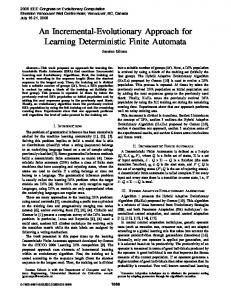
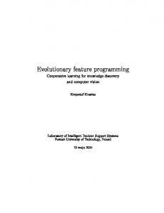
in the fourth and fifth weeks, the performance of the cat’s visual system is sharply reduced for its whole lifetime [Hubel and Wiesel, 1970]. Robots often modify their environment to communicate with each other or to ease or progress their task or navigation. For example, in [Batalin and Sukhatme, 2002] a robot is exploring an unknown environment. Such task is achieved without access to any global navigational information thanks to signposts that the robot drops off in its environment. Another example is a famous experiment with emergence, [URL - Didabots]. Robots follow a very simple algorithm – move forward until the bumper sensors are pressed, then backup, turn and start over again. Their special topology is the reason that the robots perform a useful task of grouping objects into few piles: whenever the robot meets an object in the center, its bumper sensors will not be affected, and thus the object will be pushed by the robot – until another object is encountered that will hit the bumper. Following the collision, the robot will backup and turn, and leave the object at the place of another object – in result bringing two objects together. Several robots running in an arena with many objects will group all objects into one or several groups, possibly loosing some objects along the walls. Figure 2.1 shows the implementation of our group using LEGO robotics construction sets. It is well-known that the natural intelligence has evolved through processes that involved similar simple interactions in the collonies of cells and organisms. However and more importantly, due to this evolutionary history, such interactions are very likely to be inevitable for the natural intelligence as we know it in our era. With the respect to the nature, we believe embodiness is thus necessary for any system with on-line intelligence. Both the environment and the body of a robot are equally important as its program. Another interesting example that demonstrates this is a soccer-playing robot with its ball-fallowing algorithm: the robot is moving forward and slightly turning. Whenever the ball comes out of the sight, the robot toggles the direction of the turning. Figure 2.3 shows a trajectory of a robot during the ball-following experiment using the program in Figure 2.2. When the robot is approaching the ball, even though the program is correct, the robot misses the ball in 90% of the cases on one or another side. This is due to the fact that the sensors see the ball in wide angle (giving the maximum reading), and thus the robot turns “too much” before it toggles the direction of turning. A simple modification of the robot morphology – adding an extra LEGO brick in front of the sensor as shown in the Figure 2.4 leads without modifications of the program to a successfully working solution, see Figure 2.5. Building robots and programming them are activities that need to be performed simultaneously. Technical specifications of the sensors, and robot parts are never detailed enough to allow for software implementations without the testing, adjusting, and sometimes reimplementing both the program and the robot morphology. Environment, in which an agent performs is static, when no changes in the settings occur. It is dynamic or changing when changes can occur, for example objects can be moving, changing its shape, light or magnetic conditions may change. Deterministic environments are known in advance, while the details of
22
Background
Figure 2.1: Implementation of the emergence experiment using LEGO Mindstorms. The view of the rectangular arena before and after the experiment is shown at the top, the simple program in Robotics Invention System in the center, and LDRAW/MLCAD drawing of the robot at the bottom.
2.4 Embodiment, Situatedness, Environment
23
while ( true ) { old_value = current_value; c u r r e n t _ v a l u e = S E N S O R _ 1; s e a r c h _ d i r = OUT_C ; // will start s e a r c h i n g the ball right if ( c u r r e n t _ v a l u e > t h r e s h o l d) // see the ball ? { if ( c u r r e n t _ v a l u e < o l d _ v a l u e) { // is the ball less bright than last time ? while ( true ) // follow it , until it gets lost { Fwd ( OUT_A + OUT_C ); On ( OUT_A + OUT_C ); // drives f o r w a r d until ( S E N S O R _ 1 < t h r e s h o l d) {} // until ball cannot be seen Rev ( s e a r c h _ d i r ); // turns t o w a r d s ball until C l e a r T i m e r (1); // sees ball or timer (1) > 2 until ( S E N S O R _ 1 > t h r e s h o l d || Timer (1) > 2) {} if ( S E N S O R _ 1 < t h r e s h o l d ) // if can ’t see ball , change { // d i r e c t i o n Toggle ( OUT_A + OUT_C ); // and r e m e m b e r to look for the ball // in the o p p o s i t e d i r e c t i o n next time s e a r c h _ d i r ^= OUT_A + OUT_C ; C l e a r T i m e r (1); until ( S E N S O R _ 1 > t h r e s h o l d || Timer (1) > 5) {} if ( S E N S O R _ 1 < t h r e s h o l d) // if can ’t see the ball return ; // return and start all over } } } } }
Figure 2.2: A program fragment in NQC for a soccer playing robot, which seeks and follows an infra-red ball using a single IR sensor. When the program segment is entered, the robot is already spinning left. It keeps spinning at the spot until the ball is seen. Then it still keeps spinning until the sensor reading will start to decline, i.e. it has already passed the exact direction towards the ball, when the reading has been highest. Consequently it starts driving forward towards the ball, while it is in the sight. Then it starts adjusting the direction towards it by turning to the right while moving forward, and resumes forward motion when the ball is visible again. If the ball is not found on the right-hand side, the robot toggles turning now to the left, and resumes the forward movement, when the ball is found on the left-hand side. If the ball is lost and cannot be seen neither on the left nor on the right, the routine fails, and returns. Note: Another sensor was responsible to detect whether the ball was already close to the robot. Another task running in parallel was monitoring that sensor and activated either the dribbler and the kicker as appropriate depending on the position and orientation of the robot. Better ball-following performance can be reached by using two sensors, or another sensor that can detect direction towards the IR ball, as we did in the forthcoming year. This experience provides a nice example of how morphology and code depend on each other.
24
Background
A
B
C
D
E
F
G
H
Figure 2.3: Phases of ball following of a soccer-player robot. Each phase shows the new direction of the robot from that point of time as well as where the ball is currently rolling.
Figure 2.4: Changing of the robot morphology influences the sensory capabilities. In this case, LEGO brick placed in front of the sensor reduces its sensitive angle.
2.5 Planning and Reactivity
25
Figure 2.5: The original setup that consists of an IR sensor (the five black IR phototransistors) and a single LEGO brick is shown on the left. An improved setup is shown on the right.
non-deterministic environments are a surprise for an agent. Agent performing in static and deterministic environments are naturally simpler to build and program, however, given the task, it can still be a hard engineering challenge. We (and most of AI) are concerned with agents performing in dynamic and non-deterministic environments. Having confirmed that, we can still perform studies in static or deterministic environments to learn about the methods in general.
2.5
Planning and Reactivity
A robot (or an agent) that is performing some activity or task in certain environment typically has some goals. When the agent is working itself on setting up, updating or modifying these goals, it is planning. Some agents do not plan: their behavior is constant and does not change based on the input they receive from the environment. Thus planning is an optional component of an agent. Agents, which are not planning may achieve their (fixed) goals, if their behavior is pre-configured for their environment. They can even modify their environment gradually in order to achieve more complicated goals and to trigger different parts of their fixed behavior. Planning can be performed with different degree of complexity. Some agents may be planning only a very short-term actions, while other may form complex long-term plans. Agents can perform planning of different degree of complexity simultaneously with mutual feedback between the different levels. If an agent shall perform in a dynamic and non-deterministic environment successfully, it must perceive its environment and take actions based on the percepts acquired using its sensors. Some agents may reflect to their sensory inputs based on the output of their planning module. If an agent utilizes more direct links between the sensory inputs and actuator outputs, it is reactive. Extreme view on the reactive agents requires that they do no planning, and there indeed are many examples of agents that achieve their goals without planning. These are purely-reactive agents. Agents solving more complex tasks would usually both plan and be reactive, these are often called hybrid-architecture agents in the literature as they typically
26
Background
contain features of both the traditional robotics planning systems and the features of behavior-based controllers. For an example of an architecture that is completely behavior-based, even though it performs higher cognitive functions (mapping), see the work of Mataric [Mataric, 1992]. More about the robotic architectures is in the section 2.11.
2.6
Navigation
The spatial characteristics of an agent and its environment influence the strategy for selecting and performing actions in order to move around the environment and achieve the agent’s goals: the agent navigates in its environment. These strategies, or navigation algorithms, form a separate research subarea. From simple mazeexploration strategies such as wall-following, and left/right-hand rule, to complex stochastic strategies intertwined with map-building, localization, and exploration tasks. The navigation strategy is deterministic, when the agent always chooses the same action in the same situation, and it is stochastic when the agent actions are chosen randomly (at least include some degree of randomness). Probably the most simple stochastic strategy is random movement used for environment exploration or area-cover. The robot moves for some distance along a straight line, turning randomly, bouncing or turning randomly on the area boundaries and obstacles. A nice example is one of the first autonomous lawn mower robots built by Husqvarna [Hicks II and Hall, 2000], which moves randomly on a lawn surrounded by inductive wire dug few centimeters under the ground. Such behavior results in virtually all lawn of an arbitrary shape mowed without the need of specific deterministic strategy. The cost of such a solution is a lower efficiency. However, given the robot being powered from the solar panels, this becomes a less important issue, and (as the feedback from customers suggests) it gives some entertainment value to the robot. A simple deterministic strategy for locating a target at unknown location is the depth-first search. If the location of target and the map of the environment is known, a simple shortest-path algorithm can be used. An interesting class of navigation algorithms deals with avoiding obstacles and constructing a smooth trajectory of a robot without complicated equations. In a 2D environment, a potential-fields map is constructed. Each obstacle is a source of a repulsive force vector, whereas the goal is a source of an attractive force. A composition of the force vectors in each point results in a vector of the direction of robot movement in that point. Increasing the repulsive force close to the obstacles guarantees they will be avoided, while the attractive force of the target guarantees the goal will be reached. An example of such a potential-field map is shown in Figure 2.6. A crucial role in most higher-level navigation algorithms play the landmarks. Landmarks (according to [Nehmzow, 2000]) are objects or signs that should be • Visible from various positions;
2.6 Navigation
27
Figure 2.6: A motor schema for 2D environment with 4 obstacles generated according to [Arkin, 1998] using [URL - Schemas]. The robot follows the direction of the vectors in the vector field, which is a composition of attractive force towards the target and repulsive forces from the obstacles. Motor schemas are not immune to local minima and cyclic behavior: there are locations where the robot can stall at one point, or even areas which may lead to such points.
• Recognizable under different light conditions, viewing angles, etc.; • Either stationary throughout the period of navigation, or its motion must be known to the navigation mechanism. The landmark appearance should preferably provide some unique navigational information (at least when combined with other sources of navigational information). For instance, a same kind of post on top of each hill will bear no information, while a uniquely shaped TV-tower would provide a useful landmark. In addition to local landmarks found at various locations in the environment, global landmarks – such as the Sun, stars, or stationary satellites are very useful, and biological organisms take benefit from most of them. An important theory for a class of navigational and planning algorithms are Markov Decision Problems (MDPs). MDPs are extended finite-state automata, where the transitions between states occur with certain probabilities, asserting that the probabilities of transitions in each state depend only on that state (Markovian assumption). Such a stochastic model allows for modeling the environment, sensory readings and outcome of actuator actions when these are not deterministic. States correspond to locations in the environment represented as grid-based or topological map. Alternately, states can correspond to the states of a dynamic environment, task completion progress, or the planning strategy states of an agent (for instance when modeling a behavior of an animal). In some of the states, the agent can receive
28
Background
positive or negative reward. The problem is to find a good policy for traversing the state automaton so that the reward is achieved with the highest probability. MDPs are thus closely related to the field of Reinforcement Learning, a method for learning an action-selection policy to achieve agent’s goal. Navigational algorithms often utilize the sensors for the feedback about the robot movements (this is referred to as local navigation in the literature). For instance, rotation sensors can provide information about the speed of spinning of the wheels for odometry. Using dead-reckoning, the agent estimates its location based on its own measurements of the wheels revolutions. This information can alternately be obtained or supported also using distance sensors, compass, landmark detection, or vision. Once the robot knows how much it travels, it can possibly try to locate itself within a map of the environment or try to follow, or even construct such a map (this is referred to as global navigation in the literature). An example of a global navigation algorithm used by robot Xavier [Koenig and Simmons, 1998] for pose estimation in an office environment is based on the theory of Partially Observable Markov Decision Problem (POMDP). The environment is divided into locations (states), and at each time, the robot resides at each location with a determined probability. Given the sensor and motion report, and the desired directive applied to the actuators, the probability of being at each location in the next discrete step is computed from the prior and learned model of the environment. In real robot implementations, navigation usually utilizes a combination of multiple sensory inputs (sensor fusion). For example, in [Thrun et al., 1998], the output from sonar sensors which detect the presence of obstacles is supported by scene analysis from stereo-vision. Thrun et al. demonstrate how the sonar sensors alone tend to overlook objects absorbing sound, while the vision system itself misses obstacles, which are not distinguished by their optical properties – such as glass doors, or white walls.
2.7
Sensors and Actuators
Sensors are an important source of information about non-deterministic environments. Robots operating in such environments must therefore utilize the use of sensors, which is often a difficult task given that sensory readings are usually noisy or unreliable. The robot controller thus cannot rely on a single sensory reading or it has to employ a stochastic behavior governed by stochasticity of the sensors. The most simple sensors are tactile sensors used in combination with mechanic bumpers to avoid obstacles or other objects in the environment and avoid their or robot’s damage. They however demand a physical contact. A feasible alternative are infra-red (usually short-range, 2-15 cm) or ultra-sound (usually long-range, up to several meters) proximity detectors, which detect the amount of reflected signal they emit. They are vulnerable to non-reflecting surfaces, spurious echos due to the reflections and other unexpected fluctuations in the physical properties of objects. Better precision can be achieved with laser range sensors, which can operate well also in outdoor environments.
2.8 Vision
29
Shaft encoders, or rotation sensors are used to determine the rotation speed of wheels, and can be applied to measure the distance traveled by a robot and its rotation (odometry). However, this information suffers from accumulating errors and thus has to be confronted with feedback from other sensors to align the prediction with reality. For instance, the magnetic compass sensor provides global robot orientation and thus can compensate for angular errors of robot turning. When the robot operates in large environments, GPS sensors can be used to obtain global positioning information. Another strategy for position estimation is to use the accelerometers, thus determining the actual speed of the robot in all directions. Gyroscope and tilt sensors can provide information about the robot balance, and are suitable for advanced applications, where the robot performs in threedimensional space (flight, rough terrain). Many other types of sensors exist providing usually task- or environment- specific information, such as color, temperature, humidity, atmospheric pressure, sound, radiation, altitude, etc. Of distinguished importance are visual sensor systems. Actuators allow the robot to take physical actions in the environment, or to indicate its state. These include motors, and linear elements, such as solenoids. Sound and light actuators can be used as feedback to the user, or for communication. While the most typical role of the actuators is the source of propelling movement, various specialized actuators can perform useful actions, such as welding, drilling, sweeping, gripping, lifting, etc. The basic types of motors that are suitable for experimental robotics include usual DC motors that can be driven by H-Bridge drivers, stepper motors, which allow high precision of movements, and usual modeler servomotors (often modified for full-rotation operation), which include the encoders and necessary electronics so that they can be driven by logic-level signals.
2.8
Vision
Vision is the most informative sensor system with the largest bandwidth of information. Advanced specialized algorithms have to be used to process the vision input. In its simplest form, vision can be used to trace objects discriminated by their color. Usually, however, the image must be segmented into uniform areas that form objects, their topological information together with pattern recognition and reasoning about the overall scene may eventually result in understanding of the image. Image itself provides only two-dimensional information, which itself is not sufficient for determining the distance of the observed objects. Stereo-vision uses two cameras viewing the same scene from two viewpoints, and thus allowing for distance estimation. With some drawbacks, this can be achieved by taking frames from different locations using a single camera that is moving. Computer vision is very difficult and computationally demanding, however a very active research field. Most of our experiments did not utilize any vision system as our purpose is to investigate the algorithms from their bottom application level. An up-to-date overview of relevant vision algorithms can be found in [Davies, 2005].
30
2.9
Background
Controller Architectures
A traditional approach of Artificial Intelligence (AI) uses the top-down design method, where the overall goal of the system is partitioned into sub-modules that are developed individually. When putting such modules together, there is a certain risk that the interfaces, although theoretically compatible, will in practice suffer from some unforeseen mismatch. The complexity of the robotics system is too high for a prototype-designer to be able to predict the behavior of all components accurately. It may be found during the implementation phase that a particular module cannot satisfy the physical constraints of some robot parts implied by the top-down design. Moreover, the internal architecture typically consists of a large centralized planning module with symbolic reasoning mechanisms. This module receives the sensory information, and should generate next action of the robot in every time step. However, symbolic reasoning mechanisms are generally too slow for reactive behaviors that each mobile robot tackles, in particular in case of more complex systems, where the reasoning takes into account hundreds or thousands of facts and rules. In addition, a discrete symbolic model does not necessarily suit random physical dynamic interactions that resemble natural reflexes in animals as contrasted to wise actions or answers produces by humans after a thorough logical reasoning process. Even if the technological possibilities allow building a robot according to a top-down plan, the system is very difficult to debug and maintain. In the literature, the traditional architectures are called the Hierarchical Paradigm. The controller is divided into three parts - SENSE, PLAN, and ACT. SENSE – the input component is responsible for collecting the data, ACT - is a component that drives the actuators, and PLAN is the centralized logic, sometimes monolithic, not even divided into further modules. A well known example is the robot Shakey [Nilsson, 1984]. The architectures that include planning components are sometimes called deliberative. A robot controller is responsible for selecting actions for the robot to perform, based on the current and past sensory readings and its knowledge. It is usually a combination of specialized hardware and a software running on some embedded microprocessor. In our scientific view, we are interested only in the conceptual (logical) view abstracting from the platform, implementation or other technical details. The architectures of our concern are those of bottom-up design and reactive type. Many experimental robot controllers are built as some sort of neural network. The simplest is perhaps a feed-forward NN, see for example [Floreano and Mondada, 1994]. Direct sensory inputs are fed into the layered network, the values propagate through weighted connections, and the sum of inputs in each node is usually transformed by non-linearity before the node outputs the signal to the next layer. The output signals from the last layer are sent to the robot actuators. Since this type of network cannot have an internal state, it is limited to tasks and environments that are tractable with completely reactive behavior. The connection weights can either be evolved or trained by a learning algorithm. A feed-forward NN can be extended to contain an internal state by appending
2.9 FSA as Genotype Representation
31
memory units as additional input units. They contain a copy of the outputs of nodes from previous iteration. In general, this type of architecture – recurrent NN, can achieve any type of behavior with respect to the set of computable functions. An interesting analysis of dynamics of a network that solves a simple counting task (predicting elements of sequences an bn ) can be found in [Wiles and Elman, 1995]. In ER, more popular architectures are such types of recurrent NN that contain arbitrary connections leading from any node to any other node. These include for example dynamical neural networks of Gallagher and Beer [Beer and Gallagher, 1992], in which the neuron excitations are updated in continuous time. Each neuron has its memory constant that determines the speed of activation change. The group in Sussex [Harvey, 1995] also used fully interconnected recurrent NN with binary inhibitory connections. NN were also used in modular architectures. One possibility is to allocate a separate NN for each module. In another solution (an emergent modular architecture of [Nolfi, 1997]), a single NN embraces all the modules, but the outputs consist of two values produced by selector neurons and output neurons. The function of the selector neurons is to indicate whether the situation is appropriate for the output neurons value to be taken into account. Modular NN architectures can be evolved the same way as traditional NN, or the modularity description can be contained in the genotype. A good start to the field of modular neural architectures is the overview of [Ronco and Gawthrop, 1995]. For a criticism of the use of neural architectures as a representation for EA, see for example [Steels, 1994]. Classifier Systems (CS) compose an extensive group of controller architectures for adaptive robots. They typically consist of three levels. The lowest level is an immediate control of the robot actuators based on the sensory readings and a memory. The actions are usually selected by IF-THEN rules. Second level is a learning mechanism responsible for assigning the credit to those rules that lead to a successful behavior. Rules with higher credit survive, unsuccessful rules are eliminated. CS are in this way a version of reinforcement learning and use, for example, the Bucket-brigade algorithm to propagate the credit backwards through the sequence of rules that result in the useful action of the robot. The third level is responsible for finding new promising rules and is implemented using a GA. For a review of CS, see [Wilson and Goldberg, 1989]. A very popular way of automatic controller design is Genetic Programming, [Koza, 1992b]. Typically, an action of a robot is determined by an output of one or more lisp-like S-expressions consisting of arithmetical operations and mathematical functions, constants, and special operators for sensory readings. These S-expressions are evolved by evolutionary algorithm. Special recombination operators are used, such as tree-crossover. A very first example of application of GP to robot control is in [Koza, 1992a]. Instead of S-expressions, GP techniques can be used with sequential assemblerlike programs, sets of IF-THEN or fuzzy rules [Braunstingl et al., 1995] or programs in any language, for which it is possible to generate them from definition grammar rules. More on architectures is described below in section 2.11.
32
Background
2.10
Finite-State Automata as Representation for Evolutionary Algorithms
[Fogel et al., 1995] draw a strict distinction between evolutionary approaches where the evolution is modeled as a genetic process and the approaches where the evolution is modeled as a phenotypic process. The question is the one of the representation of the individuals. Strictly seen, and pertaining to a biological relevance, the genetic processes deal with genotypes, i.e. encoding of genes that influence the shape, behavior, or other properties of the individual, whereas the phenotypic representations attempt to encode directly the complete individual, its shape, behavior and other properties in their final form. See the section 9.1.2 for a philosophical treatment of this topic. FSA or FSMs2 have been used as genotype representation in various works, although this representation lies on the outskirts of the evolutionary algorithms research and applications. Evolutionary Programming, [Fogel, 1962, 1993, 1964, Fogel et al., 1966, 1995] is a distinguished evolutionary approach that originally used FSA as the genotype representation3 . EP does not utilize recombination operators4 , and relies on mutations. The original EP works addressed the tasks of prediction, identification and control. [Chellapilla and Czarnecki, 1999] introduce modular FSMs, which are in fact equivalent to non-modular FSMs, except that the topology is restricted – in particular, the FSMs are partitioned into several encapsulated sub-parts (sub-FSMs), which can be entered exclusively through their starting states. The authors use modular FSMs to evolve controllers for the artificial ant problem that was previously successfully solved by evolving binary-string encoded FSA in [Jefferson et al., 1992]. They provide evidence that modular FSMs perform better on this task than nonmodular FSMs, and they also provide evidence that direct encoding with structural mutations of non-modular FSMs perform better than binary-string encoding used in [Jefferson et al., 1992]. This idea of modular FSMs has been adopted also by Acras and Vergilio [Acras and Vergilio, 2004], who develop a universal framework for modular EP experiments and demonstrate its use on two examples. [Angeline and Pollack, 1993] are experimenting with automatic modular emer2
The difference between FSA and FSMs in the evolutionary literature seems to be that the former refer strictly to the formal computational model as originated sometimes in the middle of the twentieth century and intensively formalized and studied for example by [Hopcroft and Ullman, 1979], while the latter usually refers to models where control actions are performed when transitions are followed. Other computer science literature, however, often makes no distinction in these two names, while various other names (Moore, Mealy) are used for different flavors of the formalism. The core of all representations, however, are the FSA, and we refer to the extensions in this article as augmented FSA, or FSA for simplicity. When referring to previous work, we attempt to use the same term as the author. 3 Further developments of EP moved from the FSA to real-value parameters representation, where the Gaussian mutation is applied to alter the parameters from generation to generation. 4 Even though later the annual EP conferences included all works relevant for Evolutionary Algorithms, and later have been integrated into Congress on Evolutionary Computation – CEC.
2.10 FSA as Genotype Representation
33
gence of FSA. They suggest to freeze and release parts of the FSA so that the frozen (or “compressed”) parts cannot be affected by the evolutionary operators. The compression occurs randomly and due to the natural selection process, it is expected that those individuals where the compression occurs for the correctly evolved sub-modules will perform better and thus compression process interacts with the evolutionary process in mutually beneficial manner. Indeed, the authors document on the artificial ant problem that the runs with compression performed better than equivalent runs without compression. They reason: “An explanation for these results is that the freezing process identifies and protects components that are important to the viability of the offspring. Subsequent mutations are forced to alter only less crucial components in the representation.” [Lucas, 2003] is evolving finite-state transducers (FSTs), which are FSA that generate outputs, in particular, map strings in the input domain with strings in the output domain. FSTs for transforming 4-chain to 8-chain image chain codes were evolved in this work, while three different fitness measures for comparing generated strings were used: strict equality, hamming distance and edit distance. An interesting piece of work by [Frey and Leugering, 2001] considers FSMs as controllers for several 2D benchmark functions and the artificial ant problem. In their representation, the whole transition function is represented as a single stronglytyped GP-tree – i.e. a branching expression with conditions in the nodes that direct execution either to the left or to the right sub-tree, and finally arriving to a set of leaves that list the legal transition pairs (old state, new state). In his PhD thesis, [Hsiao, 1997] is using evolved FSA to generate input sequences for digital circuits with the purpose of their verification, and fault detection. The author achieves best fault detection rate on various circuits (as compared to other approaches), except of those that require specific and often long sequences for fault activation. [Horihan and Lu, 2004] are evolving FSMs to accept words generated by a regular grammar. They use an incremental approach, where they first evolve FSMs for simpler grammars, and gradually progress to more complex grammars. They use the term genetic inference to refer to their approach of generating such solution. [Clelland and Newlands, 1994] are using EP with probabilistic FSA (PFSA) in order to identify regularities in the input data. The PFSA is a FSA, where the transitions are associated with probabilities as measured on input sequences. The EP is responsible for generating the topology of the FSA – number of states and how they are interconnected, and the transitions in PFSA are labeled according to their “fire rate”. This combination can be applied for rapid understanding of an internal structure of sequences. [Ashlock et al., 2002] are evolving FSMs to classify DNA primers as good and bad in simulated DNA amplification process. They evolve machines with 64 states in 600 generations. They used the weighted count of correct/incorrect classifications as their fitness function. However, they sum the classifications made in each state of FSM throughout its whole run. They argue that if only the classifications made in the final state were taken into account, the performance was poor. In addition, this allows the machine to produce weighted classification – how good/bad the classified
34
Background
primer is. The best of 100 resulting FSMs had success rate of classification of about 70%. Hybridization, i.e. seeding 1/6th of a population of an extra evolutionary run with the best individuals from 100 previous evolutionary runs improved the result to about 77%. This work was continued in [Ashlock et al., 2004], where the FSM approach was compared to more conventional Interpolated Markov Models (IMMs), which outperformed FSMs significantly. In an inspiring study from AI Center of the Naval Research Laboratory, [Spears and Gordon, 2000] analyze evolution of navigational strategies for the game of competition for resources. The strategies are represented as FSMs. Agent moves on a 2D grid while capturing the free cells. Another agent with a fixed, but stochastic strategy is capturing cells at the same time, and the game is over when there are no more cells to capture. Agents cannot leave their own territory. Authors find that the task is vulnerable to cyclic behavior that is ubiquitous in FSMs, and therefore implement particular run-time checking to detect and avoid cycles. They experiment with the possibility to disable and again re-enable states (as contrasted to permanent and complete state deletion). They also compare evolution of machines with fixed number of states and evolution of machines, where the number of states changes throughout the evolutionary run. They discover that in the case of varying number, the machines utilize the lately-added states to lesser extent, as well as that deleting states is too dramatic for performance, and thus suggest to merge or split states instead of deleting and creating states. Due to the stochastic algorithm of the opponent agent in the game of competition for resources, the fitness function must evaluate each individual in many different games (G). Authors disagree with others claiming that keeping G low can be well compensated by higher number of generations and conclude that it results in unacceptable sampling error. The authors therefore evaluate all the individuals on fewer games (500), and if the individual should outperform the previous best individual, they re-evaluate it on many more (10000) games. Some further FSM-relevant references can be found for example in the EP sections in the GECCO and CEC conferences.
2.11
Robot Programming Formalisms
Various formalisms were developed for programming robots. Some are based on standard programming languages with extensions, others are trying to look at what is special about programming robots first, and derive a formalism from such viewpoint. One of the first formalisms (used also to program the famous robot Shakey) designed as early as in 1960s that dealt with robot actions similar to behaviors were triangle tables [Nilsson, 1985]. Triangle tables are an extension of standard ruleproduction systems. They arrange the actions in a sequence, each having a list of preconditions that need to be satisfied, in order for the action to be performed. An action results in new facts to be inserted into the memory. A limited support for hierarchical organization is provided. Hierarchical organization is a weak side of the rule production systems that tend to be flat.
2.12 Behavior-Based Robotics
35
EusLisp of [Matsui and Inaba, 1999] is an object-based extension of Common Lisp with support for solid 3D modeling, concurrences, and robot manipulators. It can be conveniently used also for programming mobile robots. Task Definition Language (TDL) of [Simmons and Apfelbaum, 1998] is an extension of C++ that allows task specification and manipulation. It has been used in numerous CMU and NASA robotics projects. A compiler translates TDL code directly to C++ code. TDL features very rich set of synchronization commands, which are expressed in straight-forward manner. This makes TDL unique compared to other task-control languages. TDL is working with task trees, where nodes are associated with actions that can succeed or fail. These are either goals or commands (leaf nodes). In addition, TDL utilizes constructs for exception handling, and task monitoring (actions performed repeatedly). The programs themselves manipulate the task trees, thus the same program can generate various task trees in different runs. Microsoft Robotics Studio is a recent addition to the family of robotics languages and formalisms. It is based on Microsoft Visual Programming Language (VPL) and supports most of the currently used research architectures as well as a physics-based simulation.
2.12
Behavior-Based Robotics
A modern approach of the Nouvelle AI relies on building robots incrementally. The most trivial reactive behaviors, such as obstacle avoidance, are fully implemented, tested, and debugged first, before carefully appending higher-level behaviors. These ideas are applied in the Subsumption Architecture [Brooks, 1986]. Individual behaviors that formed the controller communicated using a fixed network, wires of which conducted simple signals. Fixed mechanisms of inhibition and suppression, and behavior priorities were used to resolve conflicts between the behaviors. Its disadvantage of hard-wiring the behaviors was addressed later in [Maes and Brooks, 1990], where individual behaviors compete for robot control and the robot can learn the conditions of applicability of each behavior in different situations. The precondition lists were learned by random trial-and-error method, and updated using relevance and reliability measures that were computed from correlation of positive (resp. negative) feedback and activity of the behavior. The research challenge that has not been studied satisfyingly well yet is whether the robot controller can be designed automatically so that it would perform some nontrivial useful task, and whether the automatic method can provide some advantages over a human-engineered solution. According to Miriam Webster dictionary, behavior is “anything that an organism does involving action and response to stimulation”. It is important that this anything, a series of interactions of the individual with its environment, is viewed from the point of view of an external observer. He or she would ask the question What will the agent achieve by doing this? This is in a sharp contrast with a point of view of an engineer who would ask the questions as: What functionality is provided by the bottom light sensor? Which components of the robot form the navigational
36
Background
cup_graspable
pickup_a_cup
analyzed_scene
search_cup
engines
navigate_to_cup
engines
cup location
gripper action
coordinate_behaviors [ pickup_a_cup(cup_graspable), search_cup(analyzed_scene), navigate_to_cup(cup_location) ] = gripper and engines action
Figure 2.7: Stimulus-response diagram (top) and functional notation (bottom) of behaviors.
unit? What are the different menu-options of the user interface? It is also important to see that this behavioral different point of view does not apply only at the very high conceptual level. Rather contrary, it is found all the way down to the signal layer of the robot controller. One can truly appreciate this when considering the automatic design of robot controllers, where the target behavior is a product of an emergent and possibly learning process instead of a result obtained by following rigid engineering standard methodologies.
2.12.1
Representing Behaviors in a Controller
A behavior-based robot controller consists of behaviors. The behaviors can be represented in different ways [Arkin, 1998]. Very common are graphical representations called stimulus-response diagrams, while functional notation is their textual counterpart. See Figure 2.7 for an example. In other formalisms, behaviors can correspond to states of a finite-state automaton (FSA), which describes sequencing of behaviors based on environmental percepts. Examples of FSA representations can be found in [Arkin and MacKenzie, 1994]. Brooks’ Subsumption Architecture also supports behaviors that are represented as augmented FSA.
2.12.2
Arbitration Mechanisms
Simultaneously performing behavioral modules all access the robot sensors and actuators. Their internal logic assumes the immediate access to the sensors and actuators. Mutual coexistence of the modules in a single robot controller must eventually lead to conflicting output values, or, perhaps, competition for bandwidth-limited inputs, or inputs that require calibration, focusing, positioning, etc. Regardless the good efforts of the designer of each individual behavioral module, combination
2.12 Behavior-Based Robotics
37
Group of behaviors (higher−level behavior)
Behavior SELECT
IN
Behavior OUT
SELECT
IN
Behavior OUT
SELECT
IN
Behavior OUT
SELECT
IN
Behavior OUT
SELECT
IN
OUT
SELECT
Behavior Arbitration
SENSOR1
SENSOR2
...
SENSORN
ACTUATOR1
ACTUATOR2 . . .
ACTUATORM
Figure 2.8: Behavior arbitration general framework. The coordination module synchronizes and prioritizes access of the behavioral modules to the robot sensors and actuators. In addition, it can send control messages to the behavioral modules (for example to turn them on and off, or to select a particular mode. Even though the diagram suggests that behavior arbitration is a centralized component, it is not necessarily so. For instance, each sensor and actuator can have its own module that synchronizes access. Similarly, each behavior can have its own arbitrator that pays attention to the overall context of the robot’s behavior and makes sure its own behavior is performing as required, receives the required inputs and delivers its output to proper destinations. That is also the approach we adopt as described in the later chapters.
of several separately functional modules in one whole will very likely result in a non-functional controller. Naturally, such a combination must be equipped with a coordination mechanism, which will enable, disable, suppress, or prioritize the input and output signals of the individual modules. The problem of action-selection or behavior arbitration must be solved in each functional behavior-based robotic controller. Figure 2.8 shows a general framework for behavior arbitration. The first proponents of the Behavior-Based Robotics suggested a fixed topology coordination with three basic coordination primitives that allow either to stop (inhibition) or replace (suppression) output signal from a behavior module on the same or lower layer in order to take priority and override the actuator output. The last primitive allows to reset the behavior to initial state. An example on Figure 2.9 shows a famous Brooks’s controller designed using Subsumption Architecture [Brooks, 1986]. Brooks’s behaviors are implemented as augmented finite-state automata (generating output, reset, inhibition, and suppression signals). As mentioned earlier, two important works on coordination mechanisms are those of [Brooks, 1986] and follow-up by [Maes and Brooks, 1990]. The combination of several behaviors can take different forms, such as independent sum, combination, suppression and sequence as studied in [Colombetti and Dorigo, 1993]. Substantial work and an overview have been done by [Pirjanian, 1999].
38
Background
Figure 2.9: An example of a controller built using the Subsumption Architecture of Brooks, [Brooks, 1987].
2.12.3
Team Robotics with Behavior-Based Architectures
Certain tasks can be completed much faster and more efficiently when a single robot is replaced by a team of multiple cooperating robots. For instance, multiple robots might observe or spot the target from different directions, they can explore environment in parallel, and they can even cooperate on transporting or capturing a large or heavy object, which would be impossible for a single robot. Unless the robots are working in a rare and precious cases of emergence, where they do not need to cooperate and when the target behavior emerges unintentionally from their simple usually random interactions, in most cases, the robots must communicate. For the same reasons as in the case of single robot system, behaviorbased architectures are suitable also for multiple robot systems. In addition, situations can occur when some behaviors run or are active simultaneously in several of the performing robots, whereas some of the robots would be taking different roles and have different behaviors active at the same time. This role distribution can take place either automatically, for example derived from the angle the robot is approaching an object to be transported, or it can be communicated and negotiated. In the latter case, the behaviors within multiple robots might use the same mechanisms for coordination across multiple robots with taking into account possible communication delays and errors. For example, in [Stroupe and Balch, 2003], a team of behavior-based robots is mapping and tracking target objects in their environment. Each robot independently determines in which direction to travel based on the current situation. Locations and observations by other robots may be communicated, but could also be inferred if teammates are detectable and their sensor models are known. When communication is absent, the full advantage of team cannot be taken until information is later
2.13 Evolutionary Robotics
39
combined. Substantial amount of work on multi-robot systems can be found in the volumes of proceedings of the International workshop on multi-robot systems.
2.13
Evolutionary Robotics
Our efforts are to combine and integrate the ideas from several independent fields. Different approaches to automatic design of robot controllers were studied. Most known are Reinforcement Learning [Sutton and Barto, 1998], [Humphrys, 1997], Neural Networks, Classifier Systems (CS) [Wilson and Goldberg, 1989], Genetic Programming (GP) [Koza, 1992b], and artificial evolution used with various controller architectures. The latter three use some form of evolutionary technique and roughly compose the sub-field of AI labeled Evolutionary Robotics, which is the main area of our interest [Beer and Gallagher, 1992], [Nolfi and Floreano, 2001], [Harvey, 1995], [Lee et al., 1998]. Most of the work in the ER field is focusing on adaptive mobile robots with neural controllers. Inspiration from biology means application of the laws of natural Darwinian evolution and motivates towards long-term evolution of individuals that successfully perform in their artificial life environment. In these cases, the focus is not on building systems that can be directly useful today or tomorrow, rather on the study of how the natural principles observed in the living species apply to the artificial robotic systems built by us. It is often not important what the agent will be able to do when the evolution completes, rather how the evolutionary process progresses, and how it interacts with the agent learning abilities. Aim is at answering the questions of how we could imitate the clever and very effective animal behavior that relies on imperfect and irregular patterns, and how to build artificial control systems that would have similar properties of the animal brains. Naturally, researchers with such motivations study controllers based on artificial neural networks, and explore various neural architectures. The systematic research efforts start and still progress with the early systems capable of obstacle avoidance, wall-following, target recognition and following, box pushing, simple autonomous flight, or survival of agents in artificial environment. It is important to point out that most (if not all) of the resulting evolved controllers perform a behavior that can easily be achieved by a manually programmed controller of small or moderate difficulty. However, the researchers in the field counter that argument by stressing their interest in adaptive and self-organizing systems, and the early stages of the research field. Briefly, ER (and EC in general) relies on evolution of population (set) of individuals (solutions to a problem). This set is usually of a fixed size. Solutions are not only good or bad, their quality (fitness) can be measured by the objective evaluation function. Objective function returns a number, which determines the quality of a solution. In the beginning of EC run, a random population is created (generation zero). Next generation is created from the previous by combining higher quality solutions and introducing few random changes into them (mutations). This requires the solutions to be encoded in some uniform way (genotype). For example, bit-strings are used in Genetic Algorithm (GA) [Holland, 1975], lisp S-expressions in
40
Background
GP or sequences of machine instructions, C-language programs [Ryan et al., 1998], etc. in other methods. EC run goes on for many generations, and the result is the best individual found during the evolution. Therefore a problem of designing a robot controller using ER method has typically the following steps (not necessarily performed in this order!): • Define the target behavior(s) that the robot will have to accomplish — the task for the robot. • Design the physical body of the robot and its hardware, decide on the sensors and actuators that the robot will use. Create a specification of signals coming from sensors and to actuators. • Decide on the controller architecture, modularity, and software platform. • Choose which of the modules and their parts can be easily designed manually and identify those which are suitable for automatic design. If there are more parts for automatic design, choose whether they will be evolved simultaneously or individually. • Find uniform encoding for automatically designed parts and define fitness (objective) functions. • Based on experience and some experiments, set up the parameters for particular evolutionary algorithm and run the evolution. • Optimize, analyze, and test the evolved parts (ideally, prove their correctness), integrate with the other parts of the controller. There are remaining open research questions. One problem is how to formally specify behaviors so that this specifications could be used automatically to generate an objective function. Another problem is how to analyze and verify the correctness of the evolved controller based on that definition later. Some researchers argue for simultaneous evolution of the robot physical topology (body) or hardware and its controller (brain) [Brooks, 1992], [Lund and Miglino, 1998]. We are mainly concerned with application of the Evolutionary Computation to the problem of design of robot controllers, as mentioned earlier in the section 2.2. A possible alternative, or rather extension, is using the EC for further adaptations during the individual’s lifetime. A systematic study of such approach can be found in the doctoral thesis of [Walker, 2003].
2.13.1
Evolvable Tasks
Although ER has been tested on many different tasks, most of them were simple. These include the following:
2.13 Evolutionary Robotics
41
• Wall following, where the robot is placed in a closed environment and has to learn navigation along the walls without collision. Robot is usually equipped with laser, sonar, or infrared proximity sensors and sometimes has a vision. • Obstacle avoidance is typically a part of some more complicated task. The goal for the robot is to navigate in the environment without running into obstacles. The environment can be static or contain moving objects. • Docking and recharging, where the robot has to find its docking station and successfully approach it. • Artificial ant following, a standard Artificial Life simulation problem. Robot is trained to follow a chemical trace by using its smell sensor. • Box pushing has several variations. A robot or a group of them are given a task of pushing box(es) to the wall, corners or specified positions. • In lawn mowing task, the robot has to move around inside of a defined arena and cover the largest possible area. The environment may contain obstacles, irregularities and moving objects. • Legged walking is used with 2,4,6,8-legged robot. The task is to train the controller to synchronize the movements of the robot. • T-maze navigation is a standard benchmark task. The robot first reads the direction at the entrance to a corridor. It has to follow the corridor to the crossing and turn right or left based on the initial instruction. • Various foraging strategies are related to Artificial Life, where the artificial environment contains food sources and the robot has to learn the strategies for finding the food. • Trash collection, is another example of searching. The robot has to pick up the trash objects, and carry them to an assigned area to drop them. • In various vision discrimination and classification tasks, the controller is trained to steer the robot depending on the vision sensory inputs. • In target tracking and navigation, the robot has to follow the target so that it remains in its vision system. • Various aspects of pursuit-evasion behaviors were also analyzed and the coevolution method was usually applied (see below). • Soccer playing robots, where the robot navigates inside a closed and deterministic environment, but interacts with other robots and the soccer ball, which has to be placed in the opponent’s gate. • Navigation tasks, where the robot needs to successfully negotiate a maze, or keep navigating in an environment with environmental clues, landmarks, beacons, etc.
42
Background
2.13.2
Fitness Space
[Floreano and Urzelai, 2000] describe a classification system for ER objective functions along three axes: • functional – behavioral axis describes whether the fitness of the individual is measured using functional properties (for instance actuator pulse frequency, robot arm position, alignment with a line, etc.) as contrasted with behavioral properties (for instance the distance traveled, number of objects collected, number of points scored, etc.) • explicit – implicit axis corresponds to the number of factors taken into account by the objective function – i.e. how much the designers tend to influence the evolutionary process towards the wished behavior (more explicit function), or leave the proper behavior to emerge naturally by keeping the number of involved criteria as low as possible. • external – internal axis refers to the types of the values utilized by the objective function: if the values can be measured directly by the sensors and internal state of the robot, the function is internal. If external observers, installations, and tools are needed, the function is external. It is claimed and we support this observation that objective functions in the aim of the designers should be as behavioral, implicit, and internal as possible. Following that advice makes the specification of the target task more human understandable, less vulnerable to errors, the search is less prone to local optima, the function is easier to implement and can be used in embedded (on-line) evolution without modifications. In addition, it appears to correspond better in an analogy to natural evolution. However, it may be more challenging to achieve good results.
2.13.3
Co-Evolution
Another common method used in ER for arranging the gradual increase of the task difficulty is the co-evolution [Cliff et al., 1992, Reynolds, 1994, Smith and Cribbs III, 1996, Juill´e and Pollack, 1996, Floreano et al., 1998]. In this approach, two simultaneous competing populations of individuals are evolved. The individuals share the same environment during their lifetime (fitness run). The individuals may have opposite goals, they can compete for the same resource, they can have the same or different roles, and optionally, they can even depend on one another in cooperation. As a consequence, the environment complexity is gradually increased over the generations as the evolution finds better individuals in both populations. The main advantage of co-evolution is that it works automatically, without the need to specify the incremental steps by a human (or machine) designer. The range of tasks amenable to co-evolution is limited. In particular, there is an inherent assumption of mutual direct or indirect interactions between the individuals in the same environment. Therefore, co-evolution applies only to evolving solutions to multi-agent problems (where the word agent is used in a broader sense, anything that actively changes its environment).
2.13 Evolutionary Robotics
43
Furthermore, co-evolution is vulnerable to stagnation due to strategy cycles, where a series of strategies relatively outperform each other in a loop. This is related to the Red Queen Effect/Hypothesis that roughly states that for an evolutionary system, continuing development is needed just in order to maintain its fitness relative to the systems it is co-evolving with. It was proposed by the evolutionary biologist [Valen, 1973]. Another issue is that co-evolution tends to generate specific solutions, which are tailored for specific strategies of the competing population, and often fails to generate robust agents that are able to perform a general strategy.
2.13.4
Evolving the Robot Morphology
The natural intelligence in the natural environment resulted after many millions of years of natural evolution. The genotype of the natural organisms influence to a large degree not only the mental and reasoning capabilities, but their physical properties alike. The intelligence of the living organisms is highly dependent on the percepts from the environment, which again are completely dependent on the mechanics, dynamics, and shape of the organisms. When the ultimate goal is a design of intelligent robots performing in natural environments using EA, it is obvious that these will have to be evolved including their morphology. The current state of the field is not yet that far due to the physical limitations (we are not yet capable of assembling robots with an arbitrary morphology), however some interesting attempts and simple experiments have been performed. A very important tool in this respect is simulation. It is therefore part of the work of evolutionary roboticist to study the possibilities of the evolution of shape, a field often called Evolutionary Design. For instance [Pollack et al., 2001] evolve various LEGO structures for a given purpose (such as crane) using a GA, later use the 3D printing machine to generate arbitrary shapes of a robotic agent, and finally evolve 2D modular locomotion machines with the help of generative grammatical representation based on Lsystems. The most interesting, as Pollack et al. show in the latter two examples, is the combination of evolving controllers and morphologies simultaneously (sometimes the term co-evolution is used also for this process). Another example is [Marbach and Ijspeert, 2004], where the morphological configuration of agents that perform locommotion is evolved together with parameters of PD controllers. Yet another interesting example are Framsticks, 3D life simulation project, developed by a group in Poznan, [Komosinski, 2003].
2.13.5
Evolving Behavior Arbitration
There have been only few attempts to generate arbitration mechanisms automatically based on the required task or robot purpose. For example, Koza [Koza, 1992a] evolves a robot controller based on Subsumption Architecture for wall-following task. He writes: “The fact that it is possible to evolve a Subsumption Architecture to solve a particular problem suggests that this approach to decomposing problems may be useful in building up solutions to difficult problems by aggregating task achieving
44
Background
behaviors until the problem is solved.” The usefulness of these approaches can be supported by the following reasons: • They are inovating: Automatic method might explore unforeseen solutions that would otherwise be omitted by standard engineering approaches used in manual or semi-automatic design performed by a human. • They can provide robot controllers with higher flexibility: Mobile robots can be built for general purpose, and the arbitration mechanism for different achievable tasks might have to be different, either for reasons of critical limits on their efficiency, the bounds on the controller capacity, or conflicting roles in different tasks. In such a case, generating the arbitration mechanism based on task description might be required. Having the option of automatic arbitration generation might save extensive amounts of work needed to hand-craft each arbitration mechanism. • They can cope with complexity: Manual arbitration design might suffer from the lack of understanding of the real detailed interactions of the robot with its environment. These interactions might be difficult to describe analytically due to their complexity. Automatic arbitration design might capture the undergoing characteristics of the robot interactions more reliably, efficiently and precisely. Learning action selection (term sometimes used interchangeably with behavior arbitration) studies in his thesis Humphrys [Humphrys, 1997]. His focus is on the “communication” of agents that together form a controller; in fact, his agents are so simple that they correspond to the nodes in a recurrent neural network, with very few control actions generated by output nodes. Input nodes receive discrete sensing of an artificial ant moving on a rectangular grid. The topology and connection weights are evolved and the communication of the very few nodes in the network is studied on a standard artificial ant seeking food in a rectangular grid problem. The most valuable inspiration for our work stems from the work of Lee et al. [Lee et al., 1998], where the more complex, high-level task is decomposed hierarchically and manually into several low-level simple tasks, which can further be decomposed to lower-level tasks. The reactive controller consists of primitive behaviors at lowest level and behavior arbitrators at higher levels, both with the same architecture of interconnected logic-gate circuit networks. The evolution proceeds from the lowest level tasks up the hierarchy to the target complex task. We see several possible improvements: • avoiding the centralized architecture, • allowing for easier modification of task by introducing a new module without affecting substantially the existing controller hierarchy, and • removing the limitation to purely reactive tasks.
2.13 Evolutionary Robotics
45
The work has been continued on by the master thesis [Ostergaard, 2000], where a football player has been evolved with the use of co-evolution. The qualitative change is in the ability to work with internal state (as contrasted to purely-reactive controllers), and more complex architecture allowing two types of arbitration: 1) a sequence of several states, and 2) selecting the module with the highest activation value; where the activation value is exponentially decreasing over time, and reset to maximum on request of the module. Even though extensibility has been slightly improved from [Lee et al., 1998] and internal state was introduced, still only a limited subclass of finite-state automata taking the arbitration role was supported. Reactive modules are not general, but have to follow with the simple unifying architecture providing only the activation level, and being based on the winner-take-all principle. Co-evolution that was used for increasing the difficulty of the evolutionary task could be applied due to the game character of the task, however it does not scale up to more general classes of tasks.
2.13.6
Incremental Evolution
A challenge of evolving a robot controller for a complex task is too difficult for a simple evolutionary algorithm. However, EC can be used for automatic controller design for more complex behaviors, if the task is divided into smaller sub-tasks. These sub-tasks can be either independent, for example individual modules that can be tested separately, or depend to some extend on other tasks – thus creating a dependence hierarchy (i.e. arranged in a tree, or in a graph). In this case, one can incrementally evolve the behaviors from the bottom of the hierarchy, and later add upper layers. This is a general framework, but various researchers already executed more concrete and specific experiments. This section’s aim is to catch most of the current and past uses of the incremental evolution. We believe that even though it is extensive, it will provide a good starting point for studying the related work about this topic. We also avoided a possible classification of the papers since there are many different viewpoints and classification criteria. An exercise of incrementally evolving a simple NN mapping of 4-bit binary vectors was presented in [de Garis, 1993]. After evolving weights for a 12-node NN for 3 binary vector pairs, 4 nodes and 1 vector pair were added to the evolved networks and the evolution continued. In the incremental case (4 vector pairs and 16 nodes), the resulting solutions had lower fitness than in a non-incremental case, which was also faster. The task was easy even for a standard GA and there was high redundancy in learning after the 3 vector pairs were already learned by part of the network. The behavior language BL for Brooks’ Subsumption Architecture was extended to a version suitable for EA called GEN. [Brooks, 1992] reasons that the robot should be initially operated with only some of its sensors, and perhaps only some of its actuators. Once the fundamental behaviors are present, additional sensors and actuators can be made available. The fitness function can vary over the time. Inman Harvey’s Species Adaptation Genetic Algorithm (SAGA) of [Harvey, 1992]
46
Background
is a modified GA that allows genotypes with variable (growing) length. The Sussex group used SAGA in experiments with incremental evolution of NN architectures for adaptive behavior, [Cliff et al., 1992]. Harvey points out that contrary to a GA, which is a general problem solving optimization and search tool working with a finite search space, SAGA fits for evolving structures with arbitrary and potentially unrestricted capabilities that require genotypes with unrestricted length. In SAGA, incremental refers to the fact that the length of the genotype increments over the evolutionary run. Typical Sussex group controllers are arbitrary interconnected networks with inhibitory and excitatory connections. Internal uniform noise is added to node’s excitation. Inhibition is binary: once a node receives at least one inhibitory signal, it does not produce any excitatory output. Certain level of excitation sets the inhibitory output of a node. Network connections are found by the evolution. SAGA has been tested on simple visually guided robot that had to remain in the center of the arena. Later, the Sussex group experimented also with increments in the task difficulty. A visually guided gantry robot learned to navigate towards a triangle in four steps: forward movement, movement towards a large target, movement towards a small target, distinguishing a triangle from a square, [Harvey et al., 1997]. Lund and Miglino incrementally evolved a Khepera robot with recurrent NN controller that performed a detour behavior [Lund and Miglino, 1998]. The task for the robot was to reach a target placed behind a U shaped obstacle. They failed to evolve such a controller non-incrementally, but succeeded with two-step process. The robot was first trained for a rectangular obstacle, which was later replaced by one of a U shape. In [Floreano, 1992], changing environment lead to better results than a static one. Authors experiment with nest-based foraging strategies of feed-forward reactive NN controllers. An environment with a constant amount of food was compared to one with decreasing amount of food, thus making the task incrementally more difficult. Environmental change caused a drastic improvement in the quality and efficiency of the foraging strategies. In the later work at Lausanne [Urzelai et al., 1998], an advanced modular architecture was trained using Behavior Analysis and Training (BAT), [Colombetti et al., 1996], [Dorigo and Colombetti, 1997]. Evolution as a global search was combined with the Reinforcement Learning during the individual’s lifetime. The robot learned to move around the arena as long as possible avoiding obstacles and regularly recharging batteries. Later the robot had to collect and deliver objects. New modules were added to the controller architecture and the genotype was augmented. Evolved parts of the genotype were masked so crossover and mutation operators did not affect them in the later stage. A group at the University of Texas, [Gomez and Miikkulainen, 1997], used incremental evolution in combination with Enforced Sub-Populations (ESP) to evolve recurrent NN architectures. Members of the population were individual neurons segregated into sub-populations. The network was formed by randomly selecting one neuron from each sub-population. Prey capture behavior of a mobile agent was evolved in 8 incremental steps. The prey, first static, was later allowed to perform several initial steps, to be finally made mobile with incrementing speed in consecutive evolutionary steps. Authors formulate heuristics for devising an
2.13 Evolutionary Robotics
47
incremental sequence of evaluation tasks. (i) Increasing the density of the relevant experiences within a trial so that a network can be evaluated based on greater information in a shorter amount of time. (ii) Making the evaluation-task easier so that the acquisition of fundamental goal-task (final task) skills is more feasible. Results of the prey capture experiments showed significantly better fitness in the case of incrementally evolved controllers compared to the direct evolution. Perkins and Hayes [Perkins and Hayes, 1996] argue that evolving NN controllers incrementally is too difficult. Their arguments are: networks with internal states are not suitable for breeding; there are difficulties with using the converged population of the previous incremental step as an initial population for the next step; protecting parts of the network responsible for behaviors learned in previous steps is impossible because these parts are not identifiable. Their Robot Shaping method is closer to a classifier system. A population of neurons that compete and cooperate to produce a behavior of a robot is evolved. The network is made up of several different species of neurons, which have different connectivity characteristics and different mutation operators. Neurons are evaluated by an analogue to the bucket-brigade algorithm from CS. In their later experiments [Perkins and Hayes, 1998] and Perkin’s Ph.D. thesis [Perkins, 1998], they evolved a target following behavior for B21 mobile robot. The task was to keep the brightest object in front, centered in its visual field. Robot was trained in two incremental steps: first only turning towards its target and later also focusing on it (pan and tilt axes). The controller consisted of several tree-like programs (agents) evolved with GP. Agents had two outputs: validity and value and they competed for the control over their assigned actuator. Before proceeding to the next evolutionary step, the current agents in the controller were frozen and the evolution continued only with appended agents. The incrementally shaped controller performed significantly better than a non-shaped, although handcrafted controller was simpler and better. A systematic study of incremental evolution in GP is in [Winkler and Manjunath, 1998]. Authors distinguish between the true incremental evolution, such as in [Lund and Miglino, 1998] from other techniques where the controller is trained in steps and previously evolved parts are held constant in subsequent steps. Authors experiment with two different termination criteria: fixed number of generations and achieving the performance limit. They employ two different population organization strategies: standard undivided population and demetic grouping, where the population consists of several isolated sub-populations that exchange the genotypes only occasionally. They statistically compare named methods applied to target tracking task of pan and tilt controlled mobile robot. Incremental evolution was used with GP in [Fukunaga and Kahng, 1995]. They evolved programs for 2 tasks. A controller for evasion in pursuit-evasion game was evolved in 2 steps: in the first step, the speed of the evader was different. They give a detailed analysis of various speeds (both slower and faster than in the final task) and time moments when the shift between the two steps occurs. They show that even a more difficult task when used as a first step, can sometimes speed-up the evolution. The reason for (problem of) this approach is that by giving a more difficult task in the beginning, the selection pressure is altered thus speeding up the evolution.
48
Background
Most likely, a similar effect can be obtained also by changing other GA parameters. In the second experiment, a controller for an artificial ant following a food trail is evolved. Authors use 2 steps: in the first step, a simpler (more difficult) trail is used. Again, authors’ results indicate that more difficult task as the first incremental step can speed up the evolution. In both experiments, they were able to evolve the required behaviors in a shorter time using incremental evolution compared to a nonincremental GP. The issue of determining effective function nodes for GP was addressed in [Naemura et al., 1998]. They successfully compare their method to ADF GP on a simulated incremental evolution on parity problem. Controllers based on fuzzy rules are evolved using incremental evolution strategy in [Hoffmann, 1998]. Evolution starts from a knowledge base containing single rule. Later, the rules are allowed to expand by either partitioning the domain of some input variable or by adding a linear term to the consequence part of the rule. More recently, active research on incremental evolution is done in AnimatLab, [Filliat et al., 1999] and [Juill´e and Pollack, 1996]. Their SGOCE paradigm evolves tree-like programs that generate recurrent NN controllers incrementally for different versions of the problem. Good solutions to a simpler version are frozen and used to seed the initial population for harder problem, where also inter-modular connections to other parts of the controller are created. For example in [Chavas et al., 1998], the group evolved a robust obstacle avoidance behavior with Khepera mobile robot in two steps, the second with a higher environmental difficulty. Impact of combining the evolution with learning in order to maintain population diversity during incremental evolution was analyzed shortly in [Eriksson, 2000] on a binary mapping task. Incremental evolution where several populations from the earlier evolutionary step are merged was used in [Desai and Miikkulainen, 2000] on the domain of the theorem proving. Neural networks were evolved to provide heuristics for constructing proofs of theorems from a simple set of axioms and two inference rules. Incremental case performed better compared to non-incremental evolution. Researchers in the field of Evolvable Hardware are facing the problem of high complexity tasks (and thus long genotypes) as well and incremental evolution comes very handy in this domain. The advantage here is that it is relatively easier to divide the task (typically a binary function) into sub-tasks. This approach (divide and conquer) was suggested and later elaborated on by [Torresen, 1999]. It was further built upon by [Kalganova, 2000], where the incremental evolution is running in two directions: from complex system to sub-systems and from sub-systems to complex system.
2.14
Simulation and Real Robotic Experiments
The proper use of simulation is a strategic topic in ER. Evaluation of evolved controllers on real robots is very time consuming. In addition, it is difficult to ensure the same conditions for evaluating the individuals in a population. Several researchers successfully demonstrated that evolution on real robots is possible
2.14 Simulation and Real Robotic Experiments
49
[Floreano and Mondada, 1994], [Floreano and Mondada, 1996]. See [Joanne Walker, 2003] for a recent comprehensive overview of evolution on real robots. Nevertheless, even very simple tasks required too many evaluations to make this approach feasible beyond trivial tasks (each individual program in each generation should be tested, preferably from several starting points, different world configurations, etc.). For example, Marc Ebner demonstrated at the EvoRobot’99 [Ebner, 1998] a wall following mobile robot equipped with sonars, with an evolved controller. GP evolution was running for two months. More reliable and human-designed program for the same task was created in few minutes! The use of simulation is accordingly necessary in most cases. The problem lies in modeling and simulating the real world accurately. The simulated sensory inputs will always differ from those obtained in the real world by real sensors. Real sensors are usually not ideal and may require calibration. In addition, EC techniques are known to be very good in finding and exploiting any unwanted regularity, and thus creating fragile solutions, which hardly transfer from simulation to reality. The traditional solution to this problem is based on adding the noise to the simulated sensory readings and combining the evaluation of individuals in simulation with evaluation on real robots. Usually, the controllers are first evolved in simulation, and later tested, tuned, or even evolved further on real robots. Real world tests can provide feedback for the simulator to modify the simulation [Brooks, 1992]. In [Lund and Miglino, 1998], the simulated sensory readings were not computed mathematically from the sensor parameters, but retrieved from look-up tables that were created by measuring the real sensors in different situations. More details on the issue of simulation in Evolutionary Robotics can be found for example in [Meeden and Kumar, 1998]. Two standard approaches to simulation can be distinguished: in a discrete event simulation, the simulation progresses in discrete steps – events, when the state of the system changes. The simulation time in discrete event simulation progresses either with constant time intervals (fixed-increment time advance simulation, also called time-slicing), or only at the occurence of state change events (next-event time advance). In the former, the events can occur only at the start of distinct units of time during the simulation – events (such as collisions, sensor readings, actuator actions) are not permitted to occur in between time units. The shorter the time unit, the more accurate is the simulation. The fixed-increment time advance simulation, however, always bears a risk for conceptual errors in the simulation outcome. For instance, when the detailed order of the occurring events is decisive, the step size must be as small as is the smallest time difference between two important events occurring. However, such short interval may be too small for the simulation to be feasible. In that case the next-event time advance simulation would be more suitable. Its disadvantage, on the other hand, is that the simulation is not updated unless some event occurs, and thus it may be difficult to follow/view the progress of the simulation. The second approach, a continuous simulation system is trying to model the exact behavior of the simulated system, its state, and the outcome of the simulation using mathematical formulas analytically, often using differential equations. In other
50
Background
Emulated program Robot OS emulator
START STOP PAUSE
Simulator of Environment
OS
Figure 2.10: The simulations in Evolutionary Robotics must simulate both the environment and the robot controller. One method is to emulate the robot controller features on the operating system of the simulating machine.
words, prediction and computation is used instead of pure observation. Analytical description of simulated system is not always possible or computable in reasonable time and thus the discrete time simulation can provide a good approximation. Simulations in ER are more complex than usual, because we simulate the behavior of a robot in its environment as contrasted to a simulation of some process that is an integral part of the simulated environment. The behavior of robot depends not only on the physical processes in the environment, but also on its own actions generated by its program – i.e. there are two simultaneous systems to be simulated. The simulation of the robot controller can be performed through direct emulation of the robot hardware/OS on the simulating hardware and OS, see Figure 2.10. That is the approach we take, more details appear in the next chapter.
2.15 Chapter Summary
2.15
51
Chapter Summary
• Robotics is a multi-disciplinary field in the overlap of the sciences and technologies of mechanics, electronics, and informatics. • Robotics has a history of more than 50 years, and it reached its very advanced stage, where robots need to act autonomously in real-world environments, and feature artificial intelligence. • Throughout the development of the field, researchers realized that building so complex systems as robots are must be done in incremental stages of multiple prototypes of increasing complexity. • Robots are performing in their environments and thus they are situated, and embodied. • A natural building block of a robotic controller is a behavior – a complete autonomous part of robot’s functionality that typically can perform on its own, and can be built, tested and debugged independently. • Behaviors share access to sensors and actuators and therefore do need to be coordinated. This coordination can take different forms. • Automatic programming of robots has been attempted either using Reinforcement Learning, or using Evolutionary Algorithms (forming the field of Evolutionary Robotics). • Simple robot behaviors have been successfully evolved. • Limited amount of work has been done on evolving the behavior coordination (behavior arbitration). • Using evolutionary algorithms to design robot controllers is very time-consuming, and therefore simulators are required. In addition, single incremental run is very limiting with respect to the task complexity. This can be overcome using co-evolution or incremental evolution.
52
Background
Chapter 3 Research Goals and Hypotheses W: Fiskeboller? P: Your smell sensor is working well. — from a conversation in the corridor of the department at 10:30 p.m. In this chapter, in the light of the assumptions described in the previous chapter, we discuss the research agenda that we seek to contribute to in the later chapters. We start with the main goals of the thesis, in particular, issues related to evolving robot controllers incrementally.
3.1
Introduction
Where does Robotics meet Computer Science? Robotics is a highly engineering and focused field with the aim to deliver compact systems capable of performing a meaningful physical activity in the real world, often with the goal to perform a useful work. The requirements for a physical entity imply that robotics is widely multidisciplinary, bringing together experts from mechanical and electrical engineering, to name the two most important. As soon as the task of the robot involves processing of any information (contrasted to a simple wired circuitry), Computer Science enters the scene. The intersections of Computer Science with Robotics thus include: • Signal Processing and Filtering • Data Clustering • Numerical Algorithms, Geometric Algorithms, Algebraic Algorithms • Pattern Recognition and Classification • Optimization • Data Compression, Communication Algorithms, Error-Correction • Search Algorithms • Planning
54
Research Goals and Hypotheses • Simulation • Machine Learning • Knowledge Representation and Processing • Human-Computer Interaction • Image Processing and Computer Vision • Embodied AI, and other fields.
It is important to understand the challenge that the high-level areas such as Artificial Intelligence, and Knowledge Representation come at the end of this list and imply mastering of the earlier fields – they can be successfully applied only after the whole thick layer of the previous sub-fields is mastered. On the other hand, they are inevitable when working on robots performing in unpredictable, dynamic, and unknown environments. Thus the AI-robotics researchers must work tightly together with the experts mastering all the areas as well with the experts in mechanical and electrical engineering, when they wish to work or research on real products. One possibility for the AI researchers to overcome the hurdle and difficult organizational challenge is to use out-of-the-box solutions of robotics systems. The option is to take a robot – an existing working finished product, and to tweak its behavior on the high level. An example of such a successful research is the work with the SONY Aibo robots. These are entertainment robots with a very advanced behavior-based controller containing about 2000 elementary behaviors that are coordinated in a messagepassing architecture – not unlike the one used in our experiments. Fortunately, SONY made the basic architecture open for user-programming, creating a splendid research platform where behaviors with access to robot sensors, vision, and actuators can be written directly in C++ and run on the robot. An interesting work has been done for instance on the language acquisition experiments [Steels and Kaplan, 2001]. Other successful and popular example of this kind is the Khepera robot [Mondada et al., 1993] that is built by experts for the purpose of research experiments. Its overall architecture is thus modular, open and prepared for experimenting with research algorithms. Our choice for a research platform, the LEGO RCX comes from the industry of entertainment and educational robotics. Its strength is in the low-cost and highflexibility of the robotics construction sets. Once the Computer Science challenges in Robotics are identified, computer scientists may revert to solving them in pure simulation, or simulation combined with testing on real robotic platforms.
3.2 Evolving Robotics
3.2
55
Evolving Robotics
Our work clearly can be categorized as Evolving Robotics1 . As contrasted to teams trying to master some robotics system completely, we are interested in narrow and innovative area that could possibly enhance robot use and design in the future. We take the starting assumption that a reasonable useful robotic system is already built and programmed. We are concerned with studying particular aspects of the adaptivity of the programming and design of the controller to make the robot successfully perform various non-trivial tasks according to user requirements. Users should be able to use our system to automatically program an existing robotic application. Our system aims at achieving this by the means of Evolutionary Computation, and maintains that the controller architecture is behavior-based. Our work classifies in the field of Evolutionary Robotics, and studies how controllers for mobile robots could be programmed in non-conventional way: automatically using task specification in form of objective function. The advantages of such an approach are: • Higher flexibility. Instead of specialized one-purpose robotic systems, more versatile systems can be produced. However, still without the requirement for a general intelligence engine, which is difficult to produce, especially with restricted resources that are available at embedded devices, such as robots. Instead, users could train their robots to perform various particular tasks, while the robot controllers would then be adjusted using an evolutionary approach. • Extensibility. Due to the behavior-based architecture and high modularity, it should be relatively simple to extend the functionality of the robotic system with additional functional modules, actuators, sensory systems, and behaviors. • Modifiability. Once the robot controller is programmed, it should be easy to switch back to learning mode and let the system generate a different controller based on the same or extended set of behaviors. • Higher efficiency. Since the robot controller is specified for a particular task, it does not have to be equipped with a general-purpose reasoning mechanism and knowledge base. It rather consists only of relevant behavioral modules in an efficient coordination. • Lower cost. The controllers designed automatically under the user’s supervision could save the time of engineering experts who would otherwise have to produce all the specialized controllers. Production costs also decrease when the same system can be applied to different tasks (i.e. larger market) as contrasted to many specialized products. • Large degree of customization. Since the users are allowed to design and train their robotic systems, they have better possibilities to design them in a manner 1
See previous chapter
56
Research Goals and Hypotheses that suits their particular needs. This would not be possible if fixed systems would be produced for the whole users group. • Open platform. The modular architecture and the possibility to add new components and modules allow for excellent open-source and open-platform availability, harnessing the potential of various contributing parts, modules, and behaviors providers. Open platforms are more likely to be robust, provide more user-friendly functionality, and have better prospects for further development, error discovery and correction.
While we study the design of robot controllers mainly in simulation, for a greater relevance, we do employ the algorithms on a real platform. This can be done only with a very limited accuracy, and using prototyping. We believe that testing our algorithms on prototypes running in the real-world can still give us valuable feedback on their performance and the issues to be carefully considered when performing the design experiments in simulation. Further sections elaborate on the flavors of Evolving Robotics in more details.
3.3
Robotic Task Complexity
Historically, the robots attached to production lines required only simple sensors and actuators, where the direct connections between them, with simple fixed control algorithms were sufficient. The more realistic the environment, the more difficult it is for the robot to exist and perform in it, perceive its state, and react to the events. Thus the complexity of the task is, for the first, influenced by the degree to which the environment is realistic – and in consequence non-deterministic, dynamic, and unpredictable. The second aspect relates to the activity the robot is required to perform – does the activity require processing a lot of input information? Is it time critical? Does it require long-term planning? How many information sources are involved? Are they conflicting or interfering? Are other agents – humans or robots involved in the activity and does the outcome depend on them? Finally, an interesting aspect of the task difficulty – especially in our context is the difficulty to describe a task: even though the environment is simple and the activity relatively easy, it might be difficult to describe. By the task description we mean the possibilities of its formalized transcription, which could be processed by an algorithm, for instance for the purposes of computing the fitness – a quantitative measure of robot performance. Another, more standard measure of task complexity could be the Kolmogorov complexity, in our case adapted as the size of the smallest FSA arbitrators that perform the required task on a BB-controller. In this context, we should notice that for each FSA (or transducer) there exists a minimal equivalent FSA (or transducer), i.e. an automaton with the minimal number of states2 . 2
This can further be hyper-minimized ??, if we can give up a limited (finite) part of the FSA functionality. That, however, is not useful in our context. We usually do not even minimize the FSA before the final population in order not to remove a potentially useful genetic material.
3.4 Arbitration Mechanisms
3.4
57
Arbitration Mechanisms
We assume that the robot builders and designers equipped the robot with a set of simple primitive behaviors. However, the robot is not [yet] able to perform any complicated tasks, where the behaviors would need to be coordinated. This is the goal of the behavior arbitration. A successful arbitration mechanism: • Should allow fast reactive responses controlled by behaviors. This implies that the modules should have as direct as possible access to the sensors and actuators. If the arbitration must coordinate their access, there must be a provision for a fast high-priority access for the critical behaviors. • Should allow confidence level for generated actions (i.e. the priority of an action will depend on how urgent it is) and this priority should provide flexibility. A behavior that may be critical in one situation may be less critical in a different situation. Various actions initiated by the same behavior may have different importance. The coordination mechanism should allow for a flexible priority. • Should be capable of taking temporal aspect into account – the actions are not instant, but take certain time – once some behavior is started, it should be finished unless an action with a higher priority overrides it. For instance, when an exploration behavior is about to perform a sequence of several movements in order to scan the environment from the current robot position, it would be undesirable to preempt it by another behavior of about the same priority (for instance a gripper positioning action, which could follow after the scanning is completed). • Behaviors should receive control feedback from arbitration – i.e. whether they were allowed to control the robot or not. The control behaviors usually depend on the feedback from their actions. This feedback can be obtained ‘cheaper’ within the arbitration than from the robot sensors. • Should allow easy modification of the existing controller by adding new functionality or exchanging some module for a similar alternative. This can be useful when robot moves to other environments or gets some part changed or upgraded. • Should ideally provide ways for easy analysis and verification. For instance, verifying that all of the parts are active and utilized during testing may exclude hidden features that could activate in novel situations, which did not occur during training and testing. • Should be easy to represent, implement in embedded devices, and amenable for evolution.
58
3.5
Research Goals and Hypotheses
Embedded Evolution
The nature of many tasks where robots might be useful requires adaptivity, learning, and dealing with unpredictable, changing and unstructured environments. It is therefore almost impossible to predict situations that the robot will have to handle during the execution of its task. Robots should be able to learn new operations and skills. Particular learning algorithms for this purpose are needed. It is becoming a real possibility to equip mobile robots with high-performance computers on-board. Their computational power can be used for much better vision and signal processing algorithms, better planning, reasoning, processing natural language commands, etc. In addition, we propose to include a simulator of the robot itself to test robot’s planned actions without the risk of failure in the real world. The simulator is used by an embedded evolutionary algorithm to evolve a good strategy or actual program code that performs a required operation. In this way, the robot can learn new skills when they become needed. A similar approach by [Grefenstette and Ramsey, 1992] is called Anytime Learning. Our approach is slightly different, namely we evolve a program for the robot instead of a set of rules; the learning component is started on demand when the novel situation is experienced and is not running all the time in the background; we don’t require real-time performance of the simulator since the robot can wait before continuing the execution of its task, although high performance of the simulator is desired as the simulation is used to compute the fitness; our model is simpler, for example it doesn’t require a feedback to simulation module provided by an execution module (which in turn requires the execution module to be fairly complex since it has to know the details of the simulation module).
3.6
Evolutionary Adaptive Mechanisms
The modern AI approaches often take inspiration from or reflect upon various processes that take place in the nature, in the biological world, and which display some similarity to the artificial problems we are attempting to solve, when an analogy can be drawn. The Evolutionary Computation as a search method takes inspiration from the search for fitting genotypes of the species living in the biosphere. In this sense, we can talk about a long-term adaptivity of species in nature, where the parallel search maintained by the whole population adapts to the changing conditions and modifies the genotype in order to improve the performance of the individuals. Most of the time, the change of the conditions occurs continuously, or at the very least, it is perceived by the species as continuous. When adopted to Evolutionary Robotics, the parallel is somewhat skewed, as it very seldom is the case that the individuals coexist together during their lifetime in a real-world environment and interact with other species, which are also experiencing a long-term adaptation. On the contrary, in most of the cases, a single individual is being tested in some simulated world with some fixed artificial conditions and discrete environment. The environment and the overall conditions typically do not change throughout the course of the evolution at
3.7 Aspects of Incremental Evolution
59
all. Exposing the individuals to changing conditions throughout the evolutionary run thus better imitates the natural processes. This suggests better performance of the incremental algorithms. The evolved individuals in nature are adapting to the changing conditions in two basic ways. In addition to the long-term adaptation mentioned above, the individuals are exhibiting a short-term adaptation, or learning. This is in most species supported by the neural system of the individual based on a neural network with high degree of plasticity of the connections. Some of the short-term adaptation can become encoded into genotype in order to produce even more fit individuals [Baldwin, 1896]. However, it is important to notice that the long-term adaptation occurs in discrete steps – the genes functioning like binary (or n-ary) switches are in concert with the environment shaping the individual’s phenotype (phenotype plasticity). In this context, evolving the weights or topologies of artificial neural networks has little biological plausibility. Considering the gene-copying and proteinproduction chemical processes and mechanisms, we argue that if a genotype encodes a set of finite-state automata that govern the behavior of the individual together with the individual behavior modules that are predefined (corresponding to fixed reflexes) and may optionally contain a learning component, we are staying closer to the ways of nature, and achieve somewhat more reasonable biological plausibility. At the same time, it has to be pointed out that the complexity of the interactions of all biological processes is so extremely high and difficult to grasp, describe and fully document and understand, that all inferences drawn from the similarity with the biosphere have to be accepted with reservations and possible objections.
3.7
Aspects of Incremental Evolution
Researchers observed in the past [Harvey, 1995] that evolving robot behavior is a hard challenge for any EA. The fitness landscape tends to be rough, and evaluation of each individual typically takes a long time. Trying to evolve more complex behaviors is often too difficult. Some groups, such as [Harvey, 1995, Lee et al., 1998] advocated the use of incremental evolution, where the complexity of the target task is decreased by decomposing it to several simpler tasks, which are easy enough to solve by an evolutionary algorithm (see [Petroviˇc, 1999] for an earlier overview of incremental evolution). We have identified five different ways, in which an evolutionary robotic algorithm can be incremental: Environment (where is the robot performing?): the earlier incremental steps can be run in a simplified environment, where the frequency and characteristics of percepts of all kinds can be adjusted to make it easier for the robot to perform the task. For instance, the number of obstacles or distance to the target can be reduced, the environment can be made more deterministic, the noise can be suppressed, landmarks can be made more visible, etc. An example of this type of incrementality is [Lund and Miglino, 1998], where box-shaped obstacles were replaced by more difficult U-shaped obstacles after the avoidance behavior for the former was evolved. Task (what is the robot doing?): the earlier incremental steps can require only
60
Research Goals and Hypotheses
part of the target task to be completed, or the robot might be trained to perform an independent simple task, where it learns skills that will be needed to successfully perform in the following tasks. An example of this type of incrementality is [Harvey, 1995], where the gantry robot evolved forward movement first, followed by stages that required movement towards a large target, movement towards a small target3 , and distinguishing a triangle from square. For another example, we might first require a football playing robot to approach the ball, later we could require also to approach it from the right direction. Controller (how is the robot doing it?): the architecture of the controller changes. For example, the final controller might contain many interacting modules, but the individual interactions can be evolved in independent steps, where only the relevant modules are enabled. In the later steps, the behavior might be further tuned to integrate with other modules of the controller. This type of evolutionary incrementality occurs seldom in the literature, but an example could be a finite-state machine-controlled robot negotiating a maze. The controller can be extended with a mapping module that is able to learn the maze topology, however, the output of the module has to be properly integrated with the output of the FSA. Nonevolutionary controller incrementality can certainly be seen in the Subsumption architecture and its flavors [Maes, 1990], and many later BB approaches. The task for the robot might require a complex controller, for example one with an internal state. Evolution can start with a simple controller that is sufficient for initial task and the controller can be extended later during the evolution. The change can be either quantitative, i.e. incrementing the number of nodes in a neural network, or qualitative, i.e. introducing a new set of primitives for a GP-evolved program. Robot sensors/actuators (with what. . . ?) the dimensionality of the search space might be reduced by disabling some of the robot sensors and actuators before they are needed for the task evolved in each particular step. An example of this can be seen in Incremental Robot Shaping of [Urzelai et al., 1998], where the Khepera robot had first evolved the abilities of navigation, obstacle avoidance, and battery recharge, before a gripper was attached to it and the robot had to evolve an additional behavior of collecting objects and releasing them outside of the arena. A subset of robot’s equipment can be used in the early steps and more specific sensors and actuators added later. Robot morphology (what form does the robot have?): the shape and size of the robot can be adjusted to make its performance better and reshaped according to final design in the later incremental steps. This kind of incrementality is also seldom seen in the literature. On the other hand, there are examples where the robot morphology itself is evolved [Lund, 2001]. We performed some work in the area of evolutionary design, which is relevant for morphology evolution. The motivation is to understand representational issues of how to efficiently encode shapes for EA. An example of morphological incrementality would be a vacuum-cleaning robot with the shape of an elliptical cylinder that needs to turn in proper direction to pass through narrow passages. It could be simplified to a circular cylinder to evolve basic navigation strategies and later updated to its final shape to achieve the proper target behavior. 3
The change of size and shape of target is environmental incrementality.
3.7 Aspects of Incremental Evolution
61
Another example is evolving the particular target shape layer by layer. We elaborate on this type of incrementality in one of our experiments. From the implementation point of view, incrementality can be achieved by modifying the simulated environment, the objective function, the genotype representation and the corresponding controller implementation, and the configuration of the simulated robot.
3.7.1
Sequential vs. Structural
When evolving the target task in multiple steps, we do not necessarily require that the steps form a linear sequence. The behavior can be partitioned into simpler behaviors in various way, and the evolution progress will follow an incremental evolution scenario graph. We provide three examples with different structure scenario graphs. These are not intended to be realistic examples rather an illustration. For example, consider a robot capable of navigating in the corridors of an office building, entering and exiting rooms through doors, and navigating within the office including climbing at clean and flat surfaces such as chairs and tables. Imagine the robot was equipped with a window-cleaning and glazing unit and we would like to automatically generate a controller that will successfully clean all windows on some floor of the office building. The robot has a set of pre-programmed behaviors that need to be coordinated for the target task. The Figure 3.1 on the left shows the predefined behavioral modules. On the right of the same figure, a possible sequential scenario for evolving the coordination of the behaviors is shown. Each next step builds on the previous step by adding new functionality. The task for the automatic design of coordination between each two steps is to activate the behaviors on the left in the proper order and dynamics to generate the behavior rewarded in the respective step. In the second example, we consider a basketball playing robot, which has the basic skills, such as dribbling, shooting, and passing implemented as behavioral modules, however, a good strategy of the player is yet to be programmed. We could generate it automatically by figuring out an effective coordination mechanism. Figure 3.2 shows the list of pre-programmed behaviors. On the right of the same figure is a possible scenario of incremental steps arranged in a tree structure. For example, the “offensive behavior” incremental step attempts to generate a good player strategy for offense depending on the number of players detected by the “track opponents” elementary behavior. It should utilize different strategies evolved in previous steps, but it can also smoothly pass from one strategy to another when the situation on the field changes. Therefore, some parts of the structures designed in the earlier steps may still be left subject of evolution in the later steps. Yet another example investigates a universal berries-picking robot that can navigate in the open-air nature with the purpose of collecting berries. There are two kinds of berries of interest – raspberries, and cloudberries – which look very similar, but grow on completely different types of plants. While raspberries grow on bushes, cloudberries grow on a 5-25 cm small plants. The robot is equipped with a small gripper, and a camera, it can navigate with the help of the vision and detect
62
Research Goals and Hypotheses
navigate inside of a corridor locate room
open door pass door
locate and enter room
climb table locate, enter room, move to window climb chair locate, enter room, move to window, wash and glaze it
soap glass glaze glass navigate inside of a room
locate and enter room, move to window, wash and glaze it, and leave the room
detect window location clean windows on the whole floor
avoid furniture
Figure 3.1: An example of scenario consisting of sequential incremental steps: window-cleaning robot.
dribble shoot pass ball catch ball
offense without an oponent from the field centre offense against one deffender offense against two deffenders
avoid defender
offense two against one
defend
offense two against two
offensive behavior
track ball defense against one track opponents
defense against two
track team−mate
defense two against one
positioning in the pitch
defense two against two
general player defensive behavior
Figure 3.2: An example of scenario of incremental steps following a tree-structure: basketball playing robot.
3.7 Aspects of Incremental Evolution
locating beries in the view
63
picking up a small round object
navigating around raspberry tree
picking up raspberry
navigating at cloudberry site
picking up cloudberry
navigating in the open−air nature site determining berry types in the location
universal berry picking detect objects in the camera view image detect free space move around operate the gripper berry detection with pattern−recognition learning
Figure 3.3: An example of scenario of incremental steps that form a directed acyclic graph: berry-collecting robot.
objects in its view. We first suggest to train the robot on picking any small objects. This behavior can then form a “seed” for both raspberry and cloudberry picking behaviors, where it merges with the respective behavior capable of navigation around the particular kind of plant. Locating berries in the view is also shared both by the navigational behavior that simply searches for berry localities, and by the picking berry behaviors. However, all behaviors are merged when the target behavior of a universal berry-picking robot is evolved – the robot navigates in the terrain, locates places with berries, navigates around and applies a correct collecting procedure. Figure 3.3 shows the list of pre-programmed behaviors and a possible scenario for automatic design of coordination. The above examples are imaginary. They are supplied only to support our explanation of how the target task can be partitioned into easier sub-tasks, where each of them can be reached by an evolutionary algorithm, while the target behavior itself would be too complex.
3.7.2
Population Transition
Another important issue is how to transfer a population from the end of one incremental step to another step. Incrementing the difficulty can be achieved either by changing the experimental setup or the fitness function. When entering a new step, already learned parts of the genotype can either remain frozen or continue to evolve. A population that converged to a solution at the end of one step might
64
Research Goals and Hypotheses
need to be reinitialized before entering another step with preserving what is already learned. Sub-parts of the problem can be either independent, for example individual modules that can be tested separately, or depend to some extent on other parts — thus creating a dependence hierarchy (i.e. arranged in a tree, or in a graph as explained above). In case of dependencies, one can incrementally evolve the behaviors from the bottom of the hierarchy, adding upper layers and parallelize the algorithm later. This is a general framework. Various researchers have already executed more concrete and specific experiments. In order to find plausible solutions, EAs require that the initial population randomly samples the search space. However, the population at the end of one step is typically converged to a very narrow area, and thus it cannot be used as an initial population in the next step. We therefore propose to generate a new initial population from several ingredients: • some portion of the original population containing the best individuals is copied, • another part is filled with copied individuals that are mutated several times, and • the remaining individuals are randomly generated. However, it is also possible to blend the populations of two or more previous incremental steps. In principle, we propose that the evolutionary incremental algorithm will take for each incremental step a full specification of blending, copying, and mutation ratios for all genome sub-parts (such as finite-state automata) and all preceding incremental steps. For example, let us examine an incremental scenario with six incremental steps. The target genome in the last incremental step consists of three finite-state automata each corresponding to one of the behavioral modules that are subject to evolution, see Figure 3.4. In addition, there may be other modules in the controller, which are already designed and which are not evolved in the particular step – these are shown filled at the figure. In our example, the second incremental step continues to evolve the automaton corresponding to the first module, and begins with evolving the automaton corresponding to module II. The third and fifth steps are completely independent, and evolve the automata for module III, and for modules I and III, respectively. The fourth and sixth step merge populations from multiple steps. Whereas the fourth step simply combines the automata for the module III coming from step 3, and automata for the modules I and II from the second step into common controller, the sixth step blends the populations from the fourth and fifth steps for both modules I and III, and further evolves the automata for the module II from the fourth step. A more complicated example could be merging one automaton from two previous steps, and another automaton in the same incremental step from two other previous steps.
3.7 Aspects of Incremental Evolution
65
1 I sensors
actuators
11 00 00 11 00 11 00 11
2 I sensors
II
3
11 00 00 11
actuators
4
II I
III
sensors
actuators
00 11 11 00 00 11 11 0000 11 11 00 00 11 00 11 00 11
00 11 11 00 11 00
III sensors
5
00 11 11 00 11 00
actuators
I
sensors
III
actuators
II I
III 6
sensors
actuators
00 11 11 00 00 11 11 0000 11 11 00 00 11 00 11 00 11
I (FSA for module I)
111 000 000 II (FSA for module II) 111
000 III (FSA for module III) 111
Figure 3.4: Population mixing in an incremental scenario.
Formally, for each module m separately, the initial population of genome parts init , originates from three types of (automata for the module m) in the i-th step, Pm,i sources: init Pm,i
=
i−1 [
init,copied init,mutated init,random (Pm,i,j ∪ Pm,i,j ∪ Pm,i,j )
j=1
which are generated based on three types of ratios describing the portion of the best ), the portion of the initial evolved population from step j to be copied (qm,i,j copied population in step i that the copied individuals will occupy (qm,i,j ), and the portion of the population in step i that will be occupied by the mutated individuals from mutated ): step j (qm,i,j
init,copied copied best Pm,i,j = extract(m, scale(best(Pjevolved , Nj qm,i,j ), Ni qm,i,j )) init,mutated mutated mutated Pm,i,j = mutate(extract(m, scale(best(Pjevolved , min(Nj , Ni qm,i,j )), Ni qm,i,j ))) init,random copied mutated Pm,i,j = rnd automaton(m, Ni (1 − qm,i,j − qm,i,j ))
where Ns is the number of individuals in the population of step s, scale(S, N) enlarges or shrinks the set S to cardinality N by sampling the individuals uniformly,
66
Research Goals and Hypotheses
best(P, N) takes the N best individuals of population P , extract(m, S) takes a set of genomes and extracts the automata for the module m, mutate(S) mutates all automata in the set S, and rnd automaton(m, N) generates N random automata for module m. init Next, all the module-specific populations Pm,i are combined into the initial init population of step i, Pi simply by combining the automata from the corresponding individuals (in the order of generation of the sets as defined above). That is, the whole incremental scenario is defined by: • the number of incremental steps: s, • the population sizes in each step: Ni , i = 1, . . . , s, • the number of modules that are subject of evolution in each step i: ki , and their lists: mi,1 . . . mi,ki , for i = 1, . . . , s, • the ratios for copying and copying with mutation, for each pair of steps i, j, copied best mutated , qm,i,j , qm,i,j . and for each module m: qm,i,j In this way, one can design an evolutionary incremental process following a scenario with a topology of a complex directed acyclic graph. However, in most of the situations, the incremental scenario does not need to be complicated and thus the number of the parameters to specify can remain manageable.
3.7.3
Emergent vs. Engineered Steps
The above scheme for specifying the incremental steps assumes that the steps are fully described and specified. The scenario is fully engineered. However, some parts of the scenario specification may be kept open. Consider, for example, a scenario with a sequential topology of incremental steps, some assignment of tasks and controller parts that are subject to evolution for each step. The algorithm will start the evolution at the highest level (target task), and recursively spawn the earlier steps when required. In this way, the algorithm may regulate the amounts of individuals copied and mutated from the earlier steps based on the need and measured learning performance of each step. In fact, the incremental steps may run in parallel, and the flow of the individuals can be perpetual as contrasted to the initial population only as our model above assumes.
3.7.4
Automatic Division into Incremental Stages
Our aim is the automatic design of the controllers. Our discussion until now did not question where does the incremental evolutionary scenario consisting of the incremental steps originate. An idealistic automatic system should provide an easy to use interface and should not require the user to specify many details or parameters. We would wish that the system would allow entering the target task in form of few sentences written in a natural language. These should be parsed and analyzed to construct a semantic
3.8 Controller Architecture Goals
67
representation referring to the robot primitive abilities, the task goals, and structure. The system should contain an extensive knowledge base that could map its concepts against the parsed representation of the target task, and allow reasoning over the target task in the terms of • constraints implied by the robot sensors, actuators, topology, and physical properties • temporal state diagram of the target task pursue • identifying the set of activities to be performed and the qualitative relations between them (reasons and consequences) The reasoning process should select a set of elementary competencies, which involve multiple modules that are to be coordinated. Depending on the granularity of the reasoning process, higher- or lower- level competencies should be generated thus devising a possible hierarchy of incremental steps, and the wished incremental scenario. Such a system would be an ultimate goal of the efforts. For the time being, we must revert back to the manually-designed prescription described in the previous sections. However, the process shall be similar in the sense of identifying the constraints and relations.
3.8
Controller Architecture Goals
In this section, we address the question of our choice of controller architecture. A task of an autonomous robot usually consists of many interactions occurring, starting, or ending at various time points. Between these events, the robot remains in some particular state. In more complex systems, this state is a juxtaposition of states of multiple simultaneous activities, which are started and finished at various times. We consider state and event to be the crucial concepts for the controller architectures of mobile robots. Many researchers advocated the use of neural network based controllers, primarily for the reasons of their high degree of flexibility, plasticity, and adaptivity. Wide class of feed-forward neural networks does not have an internal state and can only be trained for reactive behaviors, signal processing, pattern recognition, or similar. Requirement of internal state implies recurrent connections. However, the representation of states in the recurrent networks is very poorly understood. Furthermore, responsiveness of neural networks to particular events is hard to asses and analyze, and the current learning mechanisms require thousands of interactions to learn even very simple behaviors. Controllers aiming at more complex tasks must have modular architectures, but it is yet unclear how this modularity can efficiently be achieved with neural networks, and what consequences it might have on their learning rules and algorithms, see also section 2.9. We suggest studying alternative architectures, which better reflect the concepts of robot state and environmental events.
68
Research Goals and Hypotheses
upper light sensor bumper sensor
obstacle avoidance
context switching
random walk
motor driver
bottom light sensor
line following
Figure 3.5: Extensibility of the controller.
Our controller architecture is strongly inspired by BB robotics. The large numbers of interactions, which can occur at any time of robot execution arbitrarily, mean that many different activities can be triggered at any time; many different sensory inputs and their various aspects have to be monitored continuously. Instead of having one centralized learning module, BB robotics suggests distributed control in multiple behavioral modules. Our controller also consists of several independent modules, which are running simultaneously. Many of the individual interactions have to be coordinated, and the modules might need to exchange relevant information about their states. The modules communicate by sending asynchronous messages, which can be either broadcasted or sent to a specific target module. In principle, each module can access the robot’s low-level hardware (sensors and actuators), but a careful design approach leading to multiple abstract layer architectures should be taken. As a result, only very few modules (ideally one) should access each robot hardware resource and extract the relevant sensory information or synchronize the access to an actuator for all other modules. For instance, instead of having three modules access the same light sensor, we suggest there should be a single module that will do all low-level communication with the sensor, detect possibly configurable events, and inform other modules about all relevant events. The competition for robot actuators can be implemented using fixed or dynamic module priorities: the robot actuator executes an action requested by some module that has the highest priority, or becomes idle, if no module requests an action. One of the main motivations for BB robotics is the incremental building of the robot and its controller (bottom-up design). This implies the qualities labeled in the fields of software architecture as “modifiability” and “extensibility”. Indeed, to add new functionality to a working controller, it is sufficient to add a new module, and integrate it into the controller by modifying the message interface for all relevant modules to respond to the new interactions. Figure 3.5 shows an example of module addition. With the original controller, the robot randomly explores environment turning more likely towards more illuminated regions, while avoiding obstacles, until it enters the line, which it starts to follow. The added dashed module introduces new functionality: the robot will start following the line only if it is located in an area, which is illuminated. To achieve this change, the whole existing controller
3.8 Controller Architecture Goals
69
can be preserved, but the line-following controller will need to introduce a new state outside illuminated area, which can be triggered by the context switching behavior module. In this state, the line following module will not start following a line. Ideally, the message interfaces of the modules should be defined as simple and as general as possible so that each module can easily be integrated into a controller. In this way, modules can be reused across different controllers, which are built for different purposes and tasks. To extend this idea further, hardware modules, such as sensors and actuators can have certain level of intelligence and be accessed with unified interfaces so that they can be easily interchanged and configured. This idea is well adopted by LEGO robotics sets [Lau et al., 1999], and there exist other similar toolkits, such as Microbric [URL - Microbric], Parallax robotics [URL - Parallax], or [URL - Handyboard]. The idea of easy integration of intelligent sensors into larger networks is at focus for large players like Intel, or for as small groups as InnoC with their Simple Sensor Networks [URL - InnoC]. One could argue that the robot controller should be general and give the robot all the possible functionality by including all the possible behavior modules. However, the memory and CPU capacities of practical robotic systems are always limited, and thus, using separate programs (controllers) for each task, instead of insisting on one general-purpose controller, can be more feasible. To achieve generality, all the modules might be stored in a long-term memory, and only the relevant modules might be retrieved into an operational memory when a particular task is being solved. The controller thus contains a set of specific behavior modules with clearly defined message interfaces, and a coordination mechanism, which makes these modules talk together as required by a particular task. Many previous approaches to the action-selection or behavior arbitration problem are either centralized, for example [Lee et al., 1998] or too limiting, for example [Maes, 1990]. Our aim is to design a general architecture, which can cope with different design challenges in a systematic rather than an ad hoc manner. In addition, this mechanism should be easy to integrate into the set of modules that are exchanging asynchronous messages. We propose each module to have its own postmessages from other modules and sensors
messages to other modules and actuators
Post office (finite−state automaton)
Behavior module implementation
Figure 3.6: Single behavior module with its arbitrating post-office finite-state machines.
70
Research Goals and Hypotheses
office module, which filters and translates the incoming messages into the messages recognized by the module itself, and which also monitors and possibly filters or modifies the messages being sent by the module. Since the state is a central concept in the controller, we chose to first study the post-offices that have the form of finitestate automata. The state transitions are triggered by messages being received or sent by the module owning the post-office. Each state transition can result in a message being sent to the module or to other modules, see Figure 3.6. Please see also Figure 8.13 for examples of evolved FSAs and the representation of the transitions. We design our coordination mechanism as distributed, and thus gain the standard advantages of the distributed systems: robustness, modularity, better communication throughput, better encapsulation and modifiability. In particular, adding a new module to an existing controller requires only designing a new post-office for the added module and the minimum set of changes in post-offices of other modules, instead of inferring with all modules and modifying a centralized coordination mechanism. This is thanks to minimalistic interfaces, one of the standard information systems design criteria.
3.9
Simulation
Due to the need of extensive CPU resources of the Evolutionary Robotics experiments, we ought to design a simulator or use an existing one. Unfortunately, none of the existing simulators satisfied our needs, and we chose to implement our own. The following goals need to be maintained regarding simulation: • All parts of the environment that are relevant for the simulation should be included. • Simulation should be as accurate as possible. • Simulation should be as fast as possible, in order to speed-up the evolutionary run. • Simulator must provide means of quantitative feedback that can be used by the objective function to compute fitness. • The simulator must be configurable in order to perform experiments with different: – environments, – robot starting locations, – robot morphologies, – sensory capabilities of the robots, – active elements that are also part of the environment (such as changing lights). Based on these requirements, we have designed a simulator as described in the later chapters.
3.10 Chapter Summary
3.10
71
Chapter Summary
• The ultimate goal of our work is to automatically generate controllers for mobile robots performing in unstructured, changing, non-deterministic, dynamic, unpredictable environments. • The method we work with are Evolutionary Algorithms, thus we work in the field of Evolutionary Robotics. • Instead of evolving complete robot controllers, we focus on evolving the specific task functionality given the set of pre-designed behavioral modules. • Evolutionary Robotics, if it should be successful, needs some guidance, because one evolutionary run would have to deal with too large search space. • Our method for reducing the search space size is the Incremental Evolution. • The use of Incremental Evolution is not straight-forward and requires careful preparation and investigation of issues, in particular: organization of the incremental scenario, understanding the different incremental fronts: environment, task, morphology, sensors/actuators, and controller. • We attempt to evolve the arbitration mechanism for existing behaviors, ideal arbitration should be: fast and reactive, provide priorities and other confidence mechanisms, take temporal aspect into account, provide feedback to behaviors, allow easy modification, be amenable to analysis and verification, easy to implement and evolve. • The chosen formalism for the arbitration representation are finite-state automata. • The chosen controller architecture consists of simultaneously executing behavioral modules that communicate with robot hardware and with each other using message passing. • The method of studying the Incremental Evolution is by performing several realistic experiments with the chosen representation and controller architecture. These form the main focus of this thesis work.
72
Research Goals and Hypotheses
Chapter 4 Supporting Technologies In this chapter, we describe the technological domains which laid on the path to our experiments in Evolutionary Robotics. Let us look at the background technical work that was part of our efforts. In order to perform the evolutionary robotics experiments, we had to master distributed computing and RCX hardware platform. We have contributed to these fields with research work, and we gently touch these issues in this chapter.
4.1
RCX as a Research Hardware Platform
With the aim of entertainment and education, LEGO company has released a construction set containing a tiny autonomous programmable computer with sensor and motor ports and infrared serial communication port - RCX. The computer is built into a LEGO brick and thus can become a part of creative designs of various kinds that contain some degree of autonomous control. These include mobile robots that perceive their environment and decide on their actions using more or less advanced programmed controller. Software included in the set is suitable for simple programs, however, third-party programming systems allow to fully utilize the potential of the embedded CPU running on 16 MHz, and having 32KB RAM available for program and data. Stretching the original concept of the construction set a little bit, it becomes a suitable simple platform for a researcher who attempts to verify the results of the robot-simulation experiments on real hardware without extra cost and investment into particular tailor-made mechanics, hardware, or high-cost research robotic platforms. High flexibility grounded by several hundreds construction pieces allows building prototypes of virtually any robotic system. In addition, combining the set with third-party sensors and parts (compass, IR-proximity, bend-sensor, sonar, sensor multiplexer, motor-multiplexer, photo-cell, IR-light sensor) results in a sufficient set of basic parts for robot building. Low cost and the communication capabilities allow building multiple-robot systems, and trying out simple multi-robot emergent algorithms. We have designed several simple tools (programmable finite-state-automata, IRcommunication for C, Java, and original RIS software) as well as communication
74
Supporting Technologies
Figure 4.1: Reliable communication protocol between PC and RCX over an unreliable IR communication link based on confirmation, and packet-numbering as used in [Soerby, 2003]. The tokens are permanently exchanged between the communicating peers. When any side needs to send a message, it is bundled together with the next outgoing token.
protocol in a student project, where RCX was integrated together with Aibo robotics platform for a prototype for a plant safety and security analysis [Soerby, 2003], Figure 4.1. As part of another student master project, we have designed, built, and programmed a converter of IR-communication signal to radio signal transmitted over BlueTooth radio protocol, [Petroviˇc and Balogh, 2006], Figure 4.2. This allows communicating with the RCX brick in longer-range and without the requirement of visibility with the IR-tower connected to the workstation. For the reasons of unreliable IR communication of Lejos, we have designed and implemented a simple error- and erasures- correcting protocol [Petroviˇc, 2006]. Four times, we attempted to organize a nation-wide robotics soccer contest for primary and secondary schools, and sent a team or two to participate at world championship, [URL - RoboCup]. The RCX has been used in our institute as well for studies of the human-natural interfaces and for introducing the technology to pre-school children. We have done research on how RCX can interact with other entertainment robots, in particular several different robots of the WowWee family: RoboSapien, RoboPet, RoboRaptor, and others. We have designed several unique tools that allow interaction of the two robots [URL - Sapien]. These can be useful also in the educational or research contexts (for example, we used the RCX in combination with RoboSapien, web camera, and OpenCV computer vision library for target locating and chasing application [URL - CyberCamp]).
4.1 RCX as a Research Hardware Platform
75
Figure 4.2: Infra-red / Bluetooth bi-directional conversion module. The signals from the RCX are transmitted over virtual serial Bluetooth connection to PC, and viceversa. The module at the figure is connected with BlueSmirf module from SparkFun, and 9V battery (upper-left), it is shown in detail (upper-right), and the schematic designed in cooperation with Ing. Richard Balogh is shown below.
We believe, that the potential of RCX has not yet been fully discovered. The embedded CPU provides a fantastic educational platform for learning about the principles of embedded devices programming – it facilitates all usual concepts – A/D, D/A converters, timers, watchdogs, interrupts, oscillators, serial port programming, control register, rich instruction set, etc. Once present in many college and university laboratories, it can provide an excellent platform for practical exercises in embedded devices and control. Recently, we have designed a prototype of a Logo programming language (dialect of Lisp) for the new NXT programmable brick [Petroviˇc, 2007]. This moves the LEGO robotics technology to higher level, allowing interactive applications that interface Logo applications running on a PC with LEGO robotics projects.
76
4.2
Supporting Technologies
Distributed Computing
Distributed Computing harnesses the idle processing cycles of the available workstations on the network and makes them available for working on computationally intensive problems that would otherwise require a supercomputer or a dedicated cluster of computers to solve. A distributed computing application is divided to smaller computing tasks, which are then distributed to the workstations to process in parallel. Results are sent back to the master that has the role of a server, where the data are collected and delivered to the client, in the cases of master-slave client-server architectures. Alternately, the results are sent to other nodes that need them for further processing, in the cases of peer-to-peer distributed architectures. The more PCs in a network, the more processors available to process applications in parallel, and the faster the results are returned. As far as the granularity of parallelization of the application allows, a network of a few thousand PCs can process applications that otherwise can be run only on fast and expensive supercomputers. This kind of computing can transform a local network of workstations into a virtual supercomputer. Several public and popular systems for distributed computing appeared early in the 90s [Pearson, 2007]. Most of these systems, however, are either focused on some specific problems, they require dedicated hardware, or they are proprietary, offering little flexibility to developers. One class of distributed systems comprises large scale distributed computing based on thousands to millions of voluntary CPU-time donators available throughout the Internet. The users download specialized clients for their particular software and hardware platforms, and let their computers work during the unused CPU time on a particular distributed computing project, thus making their CPUs consume maximum power possible. However, these systems are typically closed for the user, who usually has little control over the code or the data being processed on his or her machine. On one hand, this is required to guarantee validity of the submitted results; on the other hand, it is a potential threat to the user’s security and trust. Such systems typically try to solve or prove some hard mathematics, bioinformatics, cryptographic or other search challenges. Examples include Folding@home, Finda-Drug, or D2 OL, helping to find oral drugs which could fight Anthrax, Smallpox, Ebola, SARS, deadly diseases for which there is currently no cure, and Malaria, a lifethreatening disease for which 40% of the World’s population is at risk. An example of a multi-purpose platform of this kind is BOINC (Berkley Open Infrastructure for Network Computing), [Anderson, 2004]. Distributed.net [URL - Distributed.net] is a very large network of users all over the world, using their computers’ idle processing cycles to run computational challenge projects, which require a lot of computing power. Examples of projects are RC5-64 secret-key, DES or CS-Cipher challenges. Another similar project is Seti@home, [URL - SETI], a scientific experiment that uses Internet- connected computers in the Search for Extraterrestrial Intelligence (SETI), by analyzing radio telescope data. The focus on very specific computational problems, and the closed code of the client makes the above mentioned systems difficult to use for our research projects.
4.3 Q2 ADP Z - Tool for Distributed Computation
77
World Community Grid [URL - World Community Grid] is a similar, but commercial version of distributed computing over the Internet. They offer a robust technology and assistance with expertise in a seamless integration into existing network environments and in a deployment of custom applications. However, many of our academic research projects cannot afford such a high cost. Another class of distributed computing systems is utilizing specialized clusters. These are typically Linux-based network-installed and booted rack-mounted powerful PCs or other workstations running software that supports distributed computing either in form of message passing, threading, sockets-based, or batch submission system. Clusters of powerful computational nodes are available to users for submitting distributed applications. An example of such cluster is the Clustis at IDI, NTNU [Cassens and Constantinescu, 2003]. A Beowulf cluster [Sterling et al., 1995] is built out of commodity hardware components, running a free-software operating system like Linux or FreeBSD, interconnected by a private high-speed network. It is a dedicated cluster for running high-performance computing tasks. The nodes in the cluster do not sit on people’s desks, they are dedicated to running cluster jobs. Distributed applications can be run on large parallel-architecture computers containing tens to thousands of CPUs. An example of such is the NTNU HighPerformance Computing project [Aerts and H. P. L¨ uthi, 2004]. Yet another class of distributed computing systems is utilizing idle CPU time of a particular institution for general purpose CPU-intensive computational tasks of its own authorized users. Universities, banks, and many other institutions are equipped with enormous unused CPU time, which they could benefit from, if they run such a system. A popular example of such a system is Condor, [Litzkow et al., 1988], a high-throughput computing environment put in force for example at the University of Oslo. The environment is based on a layered architecture that enables it to provide a powerful and flexible suite of resource management services to sequential and parallel applications. The maturity of Condor makes it very appealing for our projects, however the complexity and the restrictive license of the software make it too difficult to adapt to our requirements. A distinguished class of distributed computing is grid computing. Grids aim to give answer to all possible needs. Their approach is to provide a general-purpose environment combining all possible platforms and uses. This term is sometimes used as synonym to distributed computing, when it refers to a particular site that integrates distributed computing resources of different types under single concept. An example of such a grid is UK’s National Grid Service.
4.3 4.3.1
Q2ADP Z - Tool for Distributed Computation Motivation
In order to be able to complete the evolutionary runs required for our experiments, we must utilize multiple computers. An inexpensive way of achieving this is through the computers available in the student laboratories that are running permanently
78
Supporting Technologies
in 24 hours operation, but being used only some portion of the day. We started by running the experiments manually on the individual computers, however, a group of graduate students who all were in the need of computational power set to specify, and implement a tool that can be shared among us and others. After a summer or two, we have reached a working prototype that has various strong qualities described below.
4.3.2
Features
The design goals of the Q2 ADP Z system are ease of use at different user skill levels, inter-platform operability, client-master-slave architecture using fast message-based communication, modularity and modifiability, security of computers participating in Q2 ADP Z, and easy and automatic install and upgrade. In Q2 ADP Z, a small software program (slave service) runs on each desktop workstation. As long as the workstation is not being utilized, the slave service accepts tasks sent by the server (master). The available computational power is used for executing a task. Human system administration required for the whole system is minimal. We will now describe the features in detail.
4.3.3
User Modes
Each installation of the system requires a local administrator, who is responsible for configuring the system and installing the slave service on desktop computers, and the universal client on user computers. Individual users, however, do not need to have any knowledge about the system internals. On the contrary, they are able to simply submit their executable or interpreted (such as Lisp or Java) program from a menu-driven command-line application, where they can specify • number of runs of the application, • file path to the executable and command line arguments, • input and output files (their names are automatically generated from the run number) – either for all runs or for specified subset of runs, • directories where the files reside, • utilities to be run after individual tasks (typically to process the output files before another task is started), • maximum time allowed for a task to execute, • in what order ought the task groups be executed, • hardware (disk, memory, CPU type and speed) and software (operating system, and installed programs) requirements of the application.
4.3 Q2 ADP Z - Tool for Distributed Computation
79
1 64 5 3600 Linux i386 http://server/lib-example.so
Figure 4.3: Q2 ADP Z: A simple library-type project file. These project configuration parameters are saved into XML-structured file. The executable can be taken from a local disk or downloaded from any URL-specified address. The input and output data files are automatically transferred to slaves using a dedicated data www-server. The progress of execution can be viewed in any www-browser, see the Figure 4.8. Each run corresponds to a task – the smallest computational unit in Q2 ADP Z. Tasks are grouped into jobs – identified by a group name and a job number. System allows control operations on the level of tasks, jobs, job groups, or users. If preferred by advanced users, the project file may be edited manually or generated automatically, see the Figure 4.3 and the Figure 4.4 for examples. More advanced users can write their own client application that communicates directly with the master using API of the client service library. This allows submitting tasks with appropriate data dynamically. Finally, advanced users can write their own slave libraries that are relatively faster than executable programs and very suitable for applications with many shortterm small-size tasks, i.e. with a high degree of parallelism.
4.3.4
Inter-Platform Operability
Inter-platform operability is achieved by the pool of computers in a network that can run different operating systems and have different hardware architectures. Q2 ADP Z handles task submissions with platform specifications, and the appropriate library or executable is automatically used. At the time of writing, we have successfully tested the system on the following hardware platforms: Linux/iX86,sparc,sparc64, FreeBSD/iX86, SunOS/sun4m,sun4u, IRIX64/IP27, and Win32/iX86. Most of the code is ANSI C++ and POSIX.1 compliant and therefore porting to a new platform does not require too much efforts. We use the POSIX threads API (emulated by Windows threads on WIN32 platform).
4.3.5
Architecture
The system consists of a central process called “master”, a variable (high) number of computing processes on different computers in the network called “slaves”, and
80
Supporting Technologies
15 http://server/cgi-bin/ 7200 Win32 i386 64 5 http://server/slv_app.dll ../bin/evolve_layer.exe sphere.prj 2 50 sphere.prj sph/layout/layout.2 sph/sphere.1 sph/sphere.2 sph/sphere.3 sph/logs/evolve_layer.log.2 sph/layout/layout.1
Figure 4.4: Q2 ADP Z: Simple executable-type project file. a number of “client” processes, user applications, which generate tasks grouped in jobs. Figure 4.6 has a diagram with the overall system architecture. Slave component is run as a daemon or Windows service. Its first role is to notify the central master about its status and the available resources. These include: • operating system type • processor information: CPU type, CPU speed • physical memory available • local disk available • existing software on the local system Ready 0.5 Win32 i386 32 32 JDK GCC 129.241.102.126:9001
Figure 4.5: Q2 ADP Z: Slave status message is sent from all computational nodes in regular intervals.
4.3 Q2 ADP Z - Tool for Distributed Computation
81
input file www server www data server output file
CLIENT 1
input file executable
executable
universal slave library
user slave library
SLAVE 1
client service library
universal client
slave service
post office
post office
MASTER
universal slave library interpreter
post office
project file www server
executable manual editor
input file
interpreted user program
crypter UDP confirm
status
UDP socket
database of users
output file universal client
SLAVE 2 OS networking (Win32/UNIX)
slave service post office
universal slave library Executable
CLIENT N user client application
client service library
SLAVE M
post office
slave service post office
user slave library
Figure 4.6: Q2 ADP Z architecture.
An example of slave status message is shown at the Figure 4.5. Another role of the slave is to launch an application (task) as a consequence of master’s request. The application, in form of a library, executable, or interpreted program, is transferred from a server according to the description of the task, then it is launched with the arguments from the same task description. In case of executable and interpreted tasks, universal slave library is used. After it is launched by the slave service library, it first downloads the executable or interpreted program, either from an automatic data store (now implemented on top of www-server in Perl), or from a specified URL location. The universal library proceeds with downloading and preparing all the required input files. After the executable or interpreted program terminates, the generated output files are uploaded to the data store to be picked up later by the universal client, which originated the task. On Win32 platform, the user (or universal) slave libraries come in form of DLL module, while on UNIX platform they are dynamic libraries (this makes it difficult to port the application for example to Darwin/Mac OS, which doesn’t support dynamic libraries). The master is listening to all the slaves. This way, it has an overview of all the resources available in the system, similar to a centralized information resource center. It accepts requests for tasks from clients and assigns the most suitable computational nodes (slaves) to them. The matching is based on task and slave specifications and the history of slave availability. In addition, master accepts reservations for serial or parallel groups of computational nodes: clients are notified after resources become available. Master generates a report on current status of the system either directly on a text console – possibly redirected to a (special) file, or in form of an HTML document.
82
Supporting Technologies
client user application or universal client
client service library
2
2
Q ADPZ protocol
incoming queue
master
Q ADPZ protocol
slave user library or universal slave slave service library
post office
post office
UDPConfirm
UDPConfirm
UDPConfirm
UDPSocket
UDPSocket
UDPSocket
OS
OS
post office outgoing queue
user application protocol or Q2ADPZ universal service protocol
launch lib/exe upgrade slave system info
OS
Figure 4.7: Q2 ADP Z communication layers.
The client consists of the client service library and a client user application or the universal client application. The client service library provides a convenient C++ API for a communication with the master, allowing controlling and starting jobs and tasks and retrieving the results. Users can either use this API directly from their application or utilize the universal client, which submits and controls the tasks based on an XML-formatted project file. In version 0.6 of the system, each job needs a different client process, although we are working on extending the client functionality to allow single instance of client to optionally connect to multiple masters and handle multiple jobs. Q2 ADP Z is a free, open-source, multi-platform system with limited security for distributed computing in an IP network. It allows users to submit tasks to be computed on idle computers in the network. Q2 ADP Z design goals include user-friendliness, inter-platform operability, clientmaster-slave architecture using XML message-based communication, modularity and modifiability, and security of the computers participating in Q2 ADP Z. The latest version was successfully applied using a set of student lab computers at our department with research projects in Visualization and Evolutionary Algorithms. The structure of the implementation of the system is modular and encourages reuse of useful system components in other projects. Future development of the system will include improved support for user data security. Computation results data can be encrypted and/or signed so that the user of the system can be sure the received data is correct. This is especially useful if the system is used in an open environment, for example over the Internet. For faster performance, slave libraries can be cached at slave computers – in the current version, they are downloaded before each task is started. A flexible data storage available to other computers in Q2 ADP Z is provided by slave computers. The scheduling algorithm of the master allows for improvements. We aim at supporting more hardware platforms and operating systems.
4.3 Q2 ADP Z - Tool for Distributed Computation
83
Figure 4.8: List of slaves – status information provided by master.
The current user interface to the system is based on C++. Possible extensions of the system would be different interfaces for other languages, e.g. Java, Perl, Tcl or Python. This can easily be done, since the message exchanges between different components of the system are based on an open XML specification. The communication of the components is performed at several different layers: at the very bottom, peers exchange IP datagrams, which are inherently unreliable thus the second layer provides a reliable communication link based on packet confirmation, while the packets are optionally crypted or signed using the OpenSSL security algorithms. At the high level, the components exchange XML messages according to a protocol described in the Q2 ADP Z documentation, and the user interface provides API or program menu functionality for controlling the tasks and jobs through the user application protocol. The Figure 4.7 profiles the stack of the communication layers. We invite the interested developers in the opensource community to join our development team and we appreciate any kind of feedback. The current implementation is available from the project’s home page http://qadpz.sourceforge.net/.
4.3.6
Utilizing the Q2ADP Z for EC Experiments
To evaluate the system, we employed the version 0.6 of the system in artificial evolution of layers of 3D LEGO models [Petroviˇc, 2001a], see section 5.5. A 3D model was decomposed into individual layers. The layout of each layer, i.e. the placement of LEGO bricks was evolved by a separate task. The input and output files were automatically transferred by the universal client as specified by the project file shown at the Figure 4.4). To obtain statistically significant data,
84
Supporting Technologies
tens of independent runs were required. Q2 ADP Z installation included 70 highperformance PentiumIII/733MHz workstations located in a student laboratory. Their status is on and idle during the night, and except of the exercise deadline season approximately 30-50% idle also during the day. The Figure 4.8 shows an example status of computational progress. We received results worth many weeks of single computational time within approximately 3 days time with no configuration overhead, by simply submitting our executable to Q2 ADP Z.
4.4
Evolutionary Computation and Distributed Computing
Evolutionary algorithms (EA) are highly parallel stochastic search methods for finding approximate solutions useful when no deterministic algorithm generating good solutions is known. They are inspired by the Darwinian natural evolution principles, and work with a population (a set) of solutions that survive, mate and get mutated from generation to generation based on their performance (fitness). In each generation, all individuals in the population have to be evaluated independently. That is where it is natural to parallelize the execution of the evolutionary algorithms. Some flavors of EA work on multiple populations that evolve independently (island models) – and for them another natural place for parallelizing is allocating one (or several CPUs) for each sub-population. Alternately, evaluating a single individual can also be performed in parallel on several CPUs, if the objective function is suitable for parallelizing. Some existing EA packages support parallelization on various levels. One example is the ECJ package [Luke et al., 2005] running on the Java platform thus offering high portability across platforms. Among other features, it supports platform-independent checkpointing (which stands for automatic saving of the state of the computation for the purpose of restarting the computation from a given checkpoint) and logging, multithreading, multiple subpopulations and species, inter-subpopulation breeding, inter-process or inter-machine transfer of individuals (even across different platforms), asynchronous island models. Another popular package is the EO (evolutionary objects) implemented in C++ with templates [Keijzer et al., 2001]. It provides its own extension ParadisEO for parallelization supporting the cellular model, parallel evaluation functions, parallel evaluation, and island model. Another distributed evolutionary system DREAM [Arenas et al., 2002] is based on JEO (Java brother of EO). Its distributed computation core, DRM is independent of the EA field and can run any distributed application. Instead of master-slave or client-server architecture, they base the distributed engine on an epidemic protocol, where each node keeps a database of some of the peers in the computational network. The user of DREAM can work on several different levels depending whether the standard set of features satisfies his needs, or whether a more low-level application interface is required. For instance the user can specify its evolutionary application using simple EASEA high-level description language that is compatible also with GaLib or EO.
4.5 Distributed Evolutionary Algorithm
85
When setting up a distributed EA, one typically uses a combination of a package for distributed computation and a package for EA. The distributed computation package will be responsible for delivering the inputs/outputs to/from the computational nodes, and submitting the tasks to the nodes automatically. The user has to configure which code and data have to be processed. Usually the user specifies at how many nodes he runs a particular application, or optionally what would be the topology of the parallel virtual computer. The user can implement the communication between the computational nodes either through the shared file system, message-passing, or sockets, or simply rely on the parallelization features provided by the chosen EA package. In our case, the evolutionary robotics experiment was based on the GaLib package, which does not support parallelization, and thus we needed a distributed computing package. We chose to implement our own for the reasons of the simplicity, modifiability, control, low maintenance and installation costs, and because of the other requirements that are described in the next section.
Figure 4.9: Overall architecture of the distributed evolutionary system.
4.5 4.5.1
Distributed Evolutionary Algorithm Utilizing the Cluster Computing for EC Experiments
We have performed some of the early experiments using the group cluster ClustIS, [Cassens and Constantinescu, 2003]. This cluster utilizes a batch system for submitting tasks. The restrictions on the cluster implied that a user can submit a job that simultaneously occupies 10 CPUs, and even this was not available at various times due to multiple users in need of the computational time. In addition,
86
Supporting Technologies
our simulator used the real-time scheduling mode of Linux operating system, which is only available in the super-user mode, which in turn is not available at the common cluster. We therefore had to abandon both the idea of utilizing the group cluster and the Q2 ADP Z and seek another solution, which we describe below.
4.5.2
Universal Solution
The solution is based on the GAlib library and MySQL database. It can run either on a single computer or using any number of computational nodes, which are PCs in the student laboratories with a tailored live Linux CD (based on Knoppix 3.4 distribution). The submission of tasks to nodes and their maintaintenance is supported by UNIX shell scripts, described in [Petroviˇc, 2004].
Figure 4.10: Utilization of two versions of distributed algorithm, evaluated on 53 computational nodes on real experimental run (average of total utilization throughout all incremental steps of sequential experiment). Standard deviation for early algorithm was 0.16%, whereas only 0.05% for the improved algorithm. The utilization of the nodes is influenced by several factors: in the early algorithm, the master assigns more individuals to the same faster computational nodes (when the number of nodes does not divide the population evenly), however the speed difference does not necessarily have to be so high, and slower nodes need to wait for the faster nodes to complete the extra individual; another extreme is when the population is evenly divided and the faster nodes need to wait for the slower nodes to complete; finally, in the second algorithm, the faster nodes are doing more work, but not on the centralized request of master, but naturally thanks to their higher speed; they are therefore not necessarily more utilized, as they take on more individuals only when there is still time for it. The stand-alone implementation is using a database table with cached genomes and corresponding fitness values that were already evaluated. The distributed implementation is using a similar table for the genomes that need to be evaluated,
4.5 Distributed Evolutionary Algorithm
87
and possibly interacts with the cache, see Figure 4.9. In addition, a table listing the computational nodes that are available for computation – i.e. evaluating the genomes is used. In the distributed scenario, the evolutionary algorithm is started at N machines, where one of them works as the master node and all other machines work as slave nodes (multiple evolutionary algorithms can run simultaneously and independently – they only need to have a different identifier). The master machine has the GA object, the population, and does all the evolutionary part of work, whereas the node machines are responsible only for evaluating individuals, although they are started in the same way (except of telling them to run as slaves), and read the same configuration files. Before evaluating the population in each generation, the master machine saves all genomes to the database and marks them by ids of the slaves that should evaluate them. If cache is used, the genomes that already have been evaluated earlier are removed from the list first. Next, the slave nodes retrieve the genomes to be evaluated, and save the results back to the database. When there are no more genomes to evaluate, each slave marks that it has finished its part of the work. As soon as all the slaves have finished the work, the master node determines this and either moves all results to the cache and runs its standard fitness function, or – if cache is not used, it retrieves the newly computed fitness values from the database, and removes the records. The checkpoints, which prevent evaluation of non-promising individuals, are communicated to the slaves from the master through separate CHCKPT table – it is refilled with values in the beginning of each incremental step by master. In detail, the algorithm for the master node is as follows: run the evolutionary algorithm as the stand-alone version, with the following additions: 1. On start-up, create the slave table and TODO table 2. When the population is ready to be evaluated, it is dumped to the TODO table, and records are marked as “temporary” since they are not yet ready for evaluation by slave nodes. 3. If cache is used, remove those records from TODO table that already exist in the cache. 4. If at the beginning of new incremental step, save new checkpoint times and values to the checkpoints table 5. Retrieve list of on-line slaves and assign each slave proportional amount of remaining genomes to be evaluated (as the future work, this can be improved by assigning the amount of genomes proportional to the slave performance – thus allowing to use machines with different CPU power in the same evolutionary run). 6. Set the counts of genomes to be evaluated for all slaves in the slaves table (set the REMAINING GENOMES field) 7. Assign slave identifiers to the genome records in the table and mark them as “to do” so that the slaves start evaluating them.
88
Supporting Technologies 8. Monitor the REMAINING GENOMES values in the slaves table, as soon as they all become 0 in all records, the evaluation is finished and either all records are moved to the cache if it is in use, or they are retrieved to the memory and removed from the database. The retrieved values are collected by the master’s objective function, which returns the proper value either from the cache or directly. 9. Maintain the average time of evaluation of genomes. If some slave reaches 5-times longer time and still have not evaluated its assigned genomes, remove it from the table and assign its genomes to another slave, and continue monitoring.
10. When the evolution is finished, all records in the slave table are marked, which results in the termination of the computational nodes. 11. During the run, the algorithm state values (such as the incremental step number) are passed to the slaves through the records in the TODO table. The algorithm for the slave node is more straight forward: 1. The evolutionary algorithm is not run, only the configuration files are parsed and parameters are set. 2. After start-up, the slave waits until the slave table is created, after which it puts a record to identify itself in the slaves table. 3. It monitors the value REMAINING GENOMES in the slave table, until it becomes non-zero. 4. The slave retrieves the checkpoints from the checkpoints table. 5. The slave retrieves the genomes from the TODO table, evaluates them, and saves the fitness value back to the table, marks the genome as done, and decrements the REMAINING GENOMES counter in the slave table. 6. When the REMAINING GENOMES counter becomes zero again, continue with point 3. 7. When the slave record is deleted, terminate. Later, we have modified the distributed scenario in order to test if an improved algorithm would have a higher throughput. Instead of assigning the individuals to particular computational nodes, the master only publishes all unevaluated individuals through the database. The computational nodes individually take the individuals to be evaluated and save the fitness back to the database on the one-by-one basis. There is a little bit of communication overhead, and a little time wasted before each individual is evaluated as the slaves must make short breaks while querying the database perpetually and waiting for new individuals. On the other hand, and more importantly, slaves that proceed faster, and finish their package of individuals
4.6 Chapter Summary
89
early, are not utilized again in the earlier version of the algorithm until all slaves deliver their results. However, there still may be some individuals for which the evaluation has not been started yet. Difference lies also in the handling of the faulty slave nodes – these could be simply ignored in the new version of algorithm without the resource-demanding detection process, because the initiative is coming from the nodes, not from the master. If the result will not have been delivered back within a fixed time constant, the individual that is being evaluated by a faulty node becomes considered unallocated after that time, and another computational node will allocate it, that is, starts its evaluation. We compared the utilization of CPU nodes of the two algorithms, as shown at the Figure 4.10. The algorithm was adopted and further improved for the case of pool with computational nodes with large differences in performance by [Plavˇcan, 2007] in his master thesis that utilized distributed computing for experiments in evolutionary design.
4.6
Chapter Summary
• The hardware platform used in our experiments is the LEGO programmable sets. We have mastered this technology, made use of it for various purpose and contributed to the wide user community with several utilities. • In order to perform the evolutionary experiments, we ought to utilize Distributed Computing, in particular: • We design a distributed system for harnessing the CPU power of computers in the computer labs that we use for some of our evolutionary experiments. • For the purpose of the incremental evolution experiments, we design a specialized distributed system based on database and Unix scripts.
90
Supporting Technologies
Chapter 5 Supporting Studies In this chapter, we describe the scientific domains which laid the path to our experiments in Evolutionary Robotics. In order to better understand possible applications of Robotics – including Evolutionary Robotics and automatic design of controllers, we examine one of the application domains, Educational Robotics, in higher detail. We performed, and later discuss several studies and experiments in Educational Robotics. In our work, we are particularly interested to asses how much robotics can contribute to educational school and after-school activities, whether it is useful at all, and what are the requirements on such systems in order to bring more positive than negative outcome. Is robotics due to its costs and demands on high technological skills suitable only for the real-world applications? Can the robotics educational systems make the school classes more effective, and reach the educational goals? If yes, what form these activities can take and how they can be integrated into curriculum, who can provide the necessary instruction to meet pedagogical goals? These are serious questions that put the area into very suspicious light. Our aim in this work is to indicate several interesting ways of successful integration of the robots to curriculum and schools. As part of the overall goal of evolving robot controllers, evolving robot morphology is an important part of the problem as explained in the previous chapters. In order to be able to evolve morphology, we must first understand how to represent the shapes in evolutionary algorithms. We have contributed to these fields with research work, and we gently touch these issues in this chapter.
5.1
Role of Robotics in Education
As modern technology advances in an ever-accelerating pace, especially in the crucial fields such as computer and automation, there is a continuous demand for skilled and highly motivated workers. To ensure that this demand could be met, technology curriculum is needed at the school level to give students insight into engineering fields and attract students to technology studies. As opposed to the traditional vocational education approach, technology curriculum at the school level should discard the confined professional bias and provide an insight into engineering science [Waks,
92
Supporting Studies
1995]. Therefore, new approaches are needed to design an appropriate modern strategy for implementing high quality technology program at school level. Robotics, being a multifaceted representation of modern science and technology, fits into this planning perfectly. Realizing the potential and importance of robotics, the LEGO group has launched a range of programmable robotics products called Mindstorms in September 1998, followed up with much more powerful version in August 2006. The Mindstorms robotics base set consists of touch sensors, light sensors, rotational sensors, motors and a main building block that houses a microprocessor, which is programmable via an infrared communications port, linked to a PC. In the new version (NXT), performance and robustness have been improved, infrared communication medium was replaced by BlueTooth radio, new sensor types (sound, and ultrasonic distance sensors have been introduced) and motor actuators are more powerful with built-in encoders. Educational software RoboLab has been completely rewritten based on the collected experiences. And perhaps the most important is that the platform is open and well documented down to the low-level hardware layer.
5.1.1
Robotics in Elementary and Secondary Schools
Robotics is an engineering art combing electrical and mechanical technologies. It is widely used nowadays and has been part of our daily life. In the industrial area, robots are widely used to increase productivity and hence production capacity. Various robotic home appliances – such as vacuum cleaners, floor sweepers, lawn mowers are available on the market for competitive prices. However, due to the complexity of robotics studies, it is hard to attract and pass the knowledge to students. This can be overcome by developing interest in students at younger years by introducing the simplest robotics knowledge to them. To date, many methods have been adopted by institutions around the world to teach and develop interest in robotics among the students. However, a robotics program at school level should not only focus on the introduction of engineering skills, but should also aim to bring out the best of scientific concepts and technological principles through active, creative and meaningful learning. Robotics projects should also be able to stimulate critical thinking, communications and teamwork among students. Robotics is fundamentally an applied field and its applications affect everyday life. Focus on robotics can be an effective and exciting way for students to learn about the problem-solving strategies used by engineers in practice. In this context, the LEGO Mindstorms robotics system poses a model for creative and innovative problem solving to the complex problems attuned to contemporary industrial approaches of computer system, automation, machinery and general engineering. The potential application of Mindstorms is unlimited, as it is open-ended. To successfully manipulate the various functions of the robotics set, users need to possess integrated skills e.g. • Computer Acquisition – Programming the robot with modern computer soft-
5.1 Role of Robotics in Education
93
ware to achieve an assigned task, while addressing issues of object components interface, addressing modes, handling events, and communications. • Internet Usage – using the Internet to participate in on-line Mindstorms activities • Structuring Skill – materials, robot frames loads and stability, robot motion and collision worthiness. • Mechanics Understanding – forces and torque, differential gear, robot motion, motor shaft loading and motor control. • Electronics Understanding – light and touch sensors feedback, motor current, current loop and impedance. • Other Generic Physics Theories Understanding Mindstorms curriculum should be structured into a cooperative learning environment where small groups of students work together to maximize their own and each others’ learning. Robotics project assigned to the students could consist of multiple tasks and components, where students are given the chance for collaboration among themselves to produce work that interface and integrate well as a whole project, resembling true industrial teamwork spirit. To ensure the success of the group project, students hold each other personally and individually accountable for assigned share of the work, and appropriately use the interpersonal and small-group skills needed for cooperative efforts to be successful [Johnson et al., 1991, Smith, 1995]. Also, as Mindstorms is highly unstructured, students are encouraged to be creative in implementing solutions to complex problems that can be easily related to the real life equivalent of robotics usage or even daily automation and machinery applications.
5.1.2
Guidelines for Educators: Curriculum, Skills and Philosophy
The family of programmable LEGO products from LEGO Mindstorms and LEGO educational division (formerly known as LEGO Dacta) provide a rich set of learning materials that can encompass a wide variety of curricular activities and thinking skills. With such a wide variety of activities, students from kindergarten through college are all able to learn something from an experience with these technological tools. All students are able to dream-up an invention that is personally meaningful to them regardless of their background or gender. Teachers and researchers have used programmable bricks and their related hardware and software tools with curriculum units that include classroom systems engineering projects such as a recycling center or a town [Erwin et al., 1998], designing robotic animals [Papert, 1999], kinetic sculptures [Resnick, 1993], robotic competitions ([Oppliger, 2002], [Sklar et al., 2000], [URL - World Robot Olympiad]), scientific experimentation, and many more. Many activities fall outside the range of what people normally consider “robotics”,
94
Supporting Studies
Figure 5.1: Students from secondary school in Trondheim preparing their robot for the RoboCup Junior contest in Bremen, June 2006.
which should broaden the appeal of the LEGO system to more teachers of different disciplines ranging from art to science to technology and engineering. There are numerous thinking and social skills that are developed by designing, building, and programming with these LEGO robotics systems in a classroom setting. By using motors and sensors, students are building intuitions about such concepts as feedback and control. By programming the behavior of a robot, the student has to get inside of the mind of the RCX, and think about thinking! In other words, the student has to become an epistemologist. By constructing the mechanics of a robot, students build intuitions for concepts such as structural stability, gear ratios, and mechanical advantage. Working in groups offers an opportunity to build communication skills between partners of a project. A largescale systems engineering project involving the entire classroom can build a sense of community among the students, and touch upon diverse academic areas from researching, writing, and presenting, to science, math, architecture, and technology [Erwin, 1998]. A theoretical basis for a design-based curriculum goes back to the early progressive movement in education and such work continues today. John Dewey, famous philosopher and educational theorist, believed that a child’s natural impulses and personal interests to create, construct, and invent should provide the motivation for learning, investigating, and thinking. He laid down the foundation of a philosophy of experience. His simple yet far-reaching idea that learning happens best when beginning with direct experience is the basis for much of the “hands-on” curriculum that we see today. Constructing and creating are within the experiences of every young child, and thus is connected to their lives in a meaningful way. The LEGO system provides the perfect environment for creating the opportunities for meaningful learning. In recent years Seymour Papert and others at the MIT Media Lab have coined the phrase “constructionism” to talk about a related philosophy of
5.1 Role of Robotics in Education
95
learning. Taking the idea from constructivism that knowledge in constructed inside ones head (and not transmitted into the head like a pipeline), constructionism adds that such knowledge construction inside the head is facilitated by constructions outside of the head, be it computer programs or physical models [Papert, 1999]. In this type of education, the learning takes place in the problem-solving, ”debugging”, and engineering designing and testing [Papert, 1999].
5.1.3
Teaching-Learning Materials
Throughout the recent years, many countries adopted the vision of using robotics in schools. Robotics construction sets were purchased to thousands of primary and secondary schools, and hundreds of teachers went through series of seminars where they received first-hand experience and assistance in using the sets in the classrooms. Robotics sets are useful both at the lessons of Physics, Mathematics, and technology/IT/programming. In addition, they increase the students’ and pupils’ motivation and learning satisfaction. To program the intelligence into the Mindstorms robotics set, students would require to use computer software to design their program to be run on the robotics set. The default standard computer software that comes with the original version of the Mindstorms is RCX Code. RCX Code is a simple visual programming environment that caters for basic capabilities of Mindstorms. It enables user to visually plug programming module into each other to form a program. The educational version of Mindstorms set comes with the software ROBOLAB. There are many other high-end advanced Mindstorms programming environments developed by individual enthusiasts and groups. Most of these programming software are distributed on the Internet. Below are a few examples of these software packages: • NQC – A text-based Mindstorms programming tool based on the popular programming language C. • Bot-Kit – An interactive object oriented environment for the RCX using Smalltalk programming language. • TalkRCX – A programming interpreter for programming Mindstorms in Linux environment • Mind Control – A Visual Basic program that interprets user command text. • LegOS (BrickOS) – A real C-compiler (based on GNU GCC) that provides complete access to all RCX’s functionality and hardware, and fastest possible code. • LejOS – A Java compiler and virtual machine for RCX. RCX as an embedded device suffers from performance and memory limitations, and therefore is not very suitable for Java programming that inherently implies overhead and is not suitable for real-time performance, nevertheless, LejOS is a great tool for Java fans and programmers.
96
Supporting Studies
Educators could choose to develop their own Mindstorms software for their curricular needs since the manufacturer made available a software development kit (SDK) that makes this possible (http://www.legomindstorms.com/sdk). There are a few curricular materials available at the moment, from the official manufacturer channel and third party channel. Examples include the project of London Grid for Learning and work of [Rosenblatt and Choset, 2000]. LEGO provides a set of inspiration booklets on mechanics, buildings, energy, and robots, and a set of 16 activities with worksheets and supporting CD: Science and Technology Activity Pack. Extensive work of LDAPS team (LEGO Design and Programming System), which was at the start of RoboLab system, produced multiple creative project ideas [URL - LDAPS]. These are described also in the book [Erwin, 2001]. In her the recent book, Barbara Bratzel, a teacher at Shady Hill School, a preK through 8 independent school in Cambridge, Massachusetts, has developed a projectbased course that teaches classical mechanics through engineering [Bratzel, 2005]. Comprehensive set of materials is provided by CMU Robotics Academy [URL - CMU Robotics Academy]. Yet, there is a large potential for more curriculum material that would be easy to use for teachers without extensive previous experience and technical competence. At the college and university level, Robotics can be found not only in the study directions of automation, and robotics, but more often finds a place in other study programs, including Computer Science. For instance, at Indiana University, LEGO Robotics sets have been used in the undergraduate computer science course, [Jadud, 2000].
5.1.4
Robotics Contests
A very useful drive in the progress of robotics outside of the doors of advanced research laboratories has the origin in robotics contests. These exist at all levels – from simple local hobbyists’ meetings to large international events (for example, [URL - RoboCup], [URL - Fira], [URL - Eurobot]) and from simple-tasks such as line-following (for example, [URL - Istrobot]) to complex tasks requiring intelligent reasoning, planning, and complex navigation (for example, AAAI robotics competition). A short overview can be found for example in [Balogh, 2005], and an exhaustive list is maintained at [URL - Contests]. The competitive atmosphere of the contests contributes strongly to motivation. Figure 5.1 shows a team of Norwegian students at RoboCup Junior World championship.
5.2
Creative Educational Platforms
The importance and impact of robotics and automation systems as part of the evolution of mankind is obvious and inevitable. In order to achieve sustainable and steady progress of the technology, supply of the qualified workers is essential. In a democratic society with the freedom of choice, this can be achieved only through promoting the interest of young people in technology, and maximizing their possibilities for hands-on experiences and small scientific and technological
5.2 Creative Educational Platforms
97
projects. At the same time, researchers and teachers at the universities and other higher education institutions need suitable platforms and “microworlds”, which will allow them to easily setup student projects as well as develop and test their research contributions. As mentioned above, very popular approaches to achieve both of these goals are robotics competitions. An example is the robot football, which contributes significantly to research in the areas of multiagent systems, sensor technologies, navigation, coordination, localization, vision, and other fields. One of the advantages, but also disadvantages of many robotics contests is that the same artificial problem gets solved again and again by various groups, often reaching only a moderate level compared to already existing systems and thus limiting the positive outcome to the learning experience of the participating team. The contests have a particular engineering goal set by the rules. This restricts the student, researcher or teacher in the free experimentation. A good alternative to the contests poses the exploratory and experimental classroom work with robotics construction sets. Construction sets typically contain multitudes of tuned and well-fitting parts, sensors and actuators, which put a flexible and open tool for experimentation right on the desk of a student or a researcher. In addition to the mentioned popular LEGO Mindstorms Robotics Invention System [Lau et al., 1999], other examples include Fischertechnik [Schlottmann et al., 1997] at the level of a toy, or Parallax Robotics [URL - Parallax], or Microbric [URL - Microbric] at the level of a hobbyist or student, or Khepera robots and accessories at the level of the researcher [Mondada et al., 1993]. We propose an approach that is an alternative to the contests and construction sets: an open educational and research toolkit based on an extensible and modular ˇ drawing robot Robotnacka [Durina et al., 2006]. Our aim is to provide a platform for learning and experimentation on the introductory level, which could allow to setup interesting educational projects, and use a finally-made, precise, and well tuned robot, additional hardware accessories, and integrated software solutions – “microworlds” for constructionist learning in the subjects of mathematics, physics, algorithmics, and robotic control. Multiple instances of such robots can be exposed for free use by educators, hobbyists, and researchers in the robotics laboratory accessible through the Internet thus making the platform widely accessible for no cost. We suggest to run the robots in perpetual operation in a robotics laboratory [Petroviˇc et al., 2006], 24 hours, 7 days a week. The robots should be autonomous, powered from a rechargeable battery, and controlled remotely using built-in radio communication. The robots should perform in a maintenance-free operation. In the project of remotely-operated laboratory [Petroviˇc et al., 2006], [URL Virtuallab], see Figure 5.2, robots that were designed in cooperation with our partner were installed and are running successfully for almost 2 years of time. Robots in the laboratory are automatically recognized and connected by the server, which monitors their operation, and provides extensive functionality for both user control and protected administrator maintenance. Night operation of the laboratory is possible by means of a network-controlled light source that can be turned on and off on demand. The power source of the robot is a 6V/2.3Ah lead acid maintenancefree battery and lasts for about 2-3 hours of continuous operation. The battery
98
Supporting Studies
Figure 5.2: Viewing of the remotely-accessible robotics laboratory in a web-browser. The scene contains three robots and geometric shapes that can be detected by the camera.
is recharged automatically. With its open architecture, the laboratory has good possibilities to be used both in research educational projects [Petroviˇc, 2005] for primary and secondary schools, as well as research and project platform for both undergraduate and graduate students. It can be employed in distance learning. The laboratory is used for several undergraduate semester and diploma projects, e.g. analysis of the power sources for mobile robots, platform for development of multiagent architectures, as well as for experiments of graduate students with evolutionary and BB robotics. In the educational projects, the robots in the laboratory can be attached to the software turtle objects in the Logo programming language of a student sitting anywhere around the world. In combination with the top-view camera, the laboratory can be used as an educational tool in lessons of mathematics, physics, and programming. For instance, the software is able to detect polygon shapes, and provides a creative environment for solving constructive geometry tasks in a novel and exciting way. With the ability to move objects in the arena, the robots are a perfect platform for experiments with computer vision and artificial intelligence. The robots can work as a physical instantiation and testing platform for planning and reasoning algorithms. The exploitation of robots is also made through the Robotics introductory course at the Faculty of Electrical Engineering and Information Technology STU, [Balogh, 2007]. The programming of the robots is designed to be easy to understand and learn. For an example, Figure 5.3 depicts the portion of a C/C++ program used to make
5.2 Creative Educational Platforms
99
int r = r o b o t _ i n i t (1); // create robot object r o b o t _ u s e r(r , " john " , " turtle " ); // p r o v i d e user / passwd if (! r o b o t _ c o n n e c t (r , " 1 4 7 . 1 7 5 . 1 2 5 . 3 0 " )) // c o n n e c t the lab { printf ( " Could not c o n n e c t \ n " ); return 1; } r o b o t _ a l w a y s w a i t (r , " on " ); // set s y n c h r o n o u s mode for ( int i = 0; i < 5; i ++) { r o b o t _ f d (r , 500); // move f o r w a r d 500 steps r o b o t _ r t (r , 1152); // turn 144 d e g r e e s right ( 1 4 4 * 8 = 1 1 5 2 ) } // ( the p r e c i s i o n is 8 steps / degree ) r o b o t _ c l o s e( r ); // close the c o n n e c t i o n
Figure 5.3: Interfacing the robots in the remotely-accessible laboratory from C.
the remote robot draw a star (if the pen is inserted). Other example projects allow to control the robots with joystick, or computer mouse and even with the movements of the user’s head when looking into a camera with the use of a face recognition software. During its normal operation, the robot monitors the battery power level. When the voltage falls below an indication threshold, it notifies the server. The server chooses to wait until the user finishes the current operations, or possibly interrupts the current user and using the calibrated image navigates the robot towards determined recharging station. If there are any robots on the way, they are automatically moved away, or avoided, if they do not respond. The parking software automatically turns on illumination light and adjusts the camera settings. After the robot is docked, the parking software monitors the power level, and in the cases of a missing contact, attempts to remedy the situation by turning and re-docking. If all attempts fail, the administrator is notified by an e-mail so that a possible manual docking could be performed. The locations of the robots are determined according the yellow marks placed on tops of the robots. The parking software detects the yellow components in the image that are placed inside of black components, while it attempts to filter-out irrelevant information (the administrator can adjust various sensitivity settings so that an accurate operation is reached at various daylight conditions as well as with artificial illumination at night). Since the camera is not permanently attached to the drawing surface, but rather mounted on an independent stand, the software automatically detects the position, and zooming aspect of the camera relative to the surface in order to calculate proper locations and thus the distances and angles in the position commands given to the robots when approaching the recharging station. All parts of the server side software are open-source and publicly available at the project website [URL - Virtuallab]. Interested developers are encouraged to contact us and join the development team.
100
5.3
Supporting Studies
Ten Educational Projects
The technological progress, our robot attempting to be an example of, can be meaningful, only if the technologies improve our lives, and work. Our way of improving the lives of the students is increasing their chances for learning the curriculum material by making it more understandable, motivating, active, entertaining, closer to the real world, challenging, suitable for group project learning, and stimulating constructive and exploratory thinking. For this purpose, we have developed 10 one-lesson projects and curriculum materials that can be used by teachers and students without any technical knowledge. Math Projects Circles. Even though the geometric precision of a turtle when drawing straight lines is limited by natural laws (a difference of 0,01 mm in the wheel diameter results in an error in the magnitude of centimeters when the robot draws only a square with the side length 1 m; imprecision can be somewhat compensated by robot calibration, but imperfections have to be expected), this does not apply to circles. Indeed, the turtle can draw quite precise circles. To many of us, it can be surprising to learn that the result of the command r’ltspeed 30 70, which sets the speed of the left and right wheels to -30 and +70 respectively, results in a clean circle. In the circles projects, the students learn the circle properties, and in a sequence of exercises draw circles of arbitrary diameter with their robot turtle. Triangles. Triangles are the simplest closed shapes a turtle can draw, but they provide a plethora of interesting challenges and exercises, where the students test their knowledge of triangles. From computing the angles and sides given various parameters (thus employing various theorems), constructing tangents and heights, lesson continues through drawing and understanding circumscribed and inscribed circles. Triangles can be constructed of colored insulating tape on the whiteboard surface, if the camera system is installed, or alternately, defined on the student screen only. Sets of points. Line is a half of a set of points that have a constant distance from another line, a circle is a set of points with a constant distance from a point, a parabola is. . . In this lesson, students acquire scene using the vision system and construct various sets of points that share certain property, such as distance to a vertex, distance to multiple shapes, and difference of distances. Students work with high-level concepts, shapes, and points when constructing programs to navigate the drawing robot. Constructive geometry. This lesson is based on a micro-world environment that defines a set of geometric construction operations. These differ from the standard constructive geometry with ruler and compass. The program can acquire the scene, label the points, divide line segments, determine the distances, and angles. The micro-world environment allows the teacher to define his or her own tasks, and to specify the set of available commands for each task separately. Therefore the students are required to find a creative solution given a very simple command set, instead of directly computing the target location, for instance.
5.3 Ten Educational Projects
101
Figure 5.4: Solution to the example 1.
Figure 5.5: Solution to the example 2.
Example 1: Construct a quadrangle, given the side a=650, all internal angles α = 67o , β = 90o , δ = 105o , and the diagonal e = 800. The robot pen is down. Use the commands lt, fd, defpoint, and fdupid (fd until point is in certain distance). Example 2: Given is a point A and two non-parallel lines that intersect outside of the whiteboard. Draw a line that connects A with the intersection of the two lines. The robot pen is up, and it is located somewhere outside the lines, heading towards both of them, intersecting them sufficiently far from the area boundaries. Use the commands fdul (forward until line), defpoint, fd, heading2pt, followline.lt, fduhtp (fd until heading to point), pd, moveto. The micro-world environment provides more than 30 high-level predefined commands that can be selected for particular tasks. The teacher users are very welcome to define more operators. More examples and the commands reference can be found in the Logo application for Robotnacka. Algorithmic Projects Convex hull. The camera system and cv4logo detects the list of points of all polygons placed on the whiteboard. Students are instructed to construct programs that draw
102
Supporting Studies
Figure 5.6: View from the top-mounted camera (left), the same image recognized by the image recognition plug-in for Imagine (middle), drawing a convex hull (right)
convex hulls in cooperation with teacher and using high-level constructs – from specific and simple cases towards a general case that concludes the exercise, see Figure 5.6 Depth-first search. A maze formed of black insulating tape attached to the whiteboard contains marked locations. Robot uses the sensors to read the marks encoded in binary notation (number and position of black stripes). The task for the students is to make the robot locate the target location (place for the robot parking, or unloading an object) by writing a simple Logo program that will negotiate the maze. Minimum spanning tree. The vision system detects locations of cities depicted by circles placed over the whiteboard. Students learn about the problem of the minimum spanning tree construction and develop a Logo program for the robot that makes it draw the minimum spanning tree. Students experiment with and evaluate the heuristics for tree-drawing sequencing. Polygon triangulation. In this advanced project, the students construct a single algorithm for arbitrary polygon triangulation. The task for the robot is to draw the triangulation of a polygon detected by the vision system. The exercise starts with simple convex polygons and extends to general non-convex polygons. Physics Projects Collisions. A turtle robot moving at a controlled constant velocity meets an object in an elastic or inelastic collision. In this laboratory exercise the students learn about the collision physics, measure the velocities using the camera after they calibrate it, and compare their measurements with the computed prediction. At the end, they produce a polished lab report. Force, power, friction, and work. The more slowly the robot is moving, the stronger force it can generate. For instance, it can push a heavier object, or extend a spring of a Newton-meter (and the more battery power it consumes as well). This is the property of the stepper-motor drive. Students measure the velocity decline either by marks drawn by the robot, or using the top-mounted camera. In this lesson, they review their previous knowledge of force, power, and energy physics laws and
5.4 Evolve with Imagine – Educational Evolutionary Environment
103
apply it in the set of exercises. Using the computations based on measurements, they compute the friction coefficients for different materials, speeds, and pressures.
5.4
Evolve with Imagine – – Educational Evolutionary Environment
Imagine Logo is a full-fledged functional interpreted programming language – a dialect of Lisp developed for teaching programming in the schools. As such, it has strong support for graphics and visualization, objects, and easy data manipulation, and therefore it is suitable as fast prototyping tool. Since one of our goals is to study the use of robotics in the educational process, and another – more central goal is to study the evolution of robot controllers, Imagine Logo provides an excellent platform to combine the two goals. It contains the support for controlling both LEGO robots (RCX), and the Robotnacka platform that we used in other experiments (see section 5.2). EI implements the two representation types described in the section 6.1.1, as well as the third representation type – weighted FSA (labeled HMM due to its similarity to Markov Models), where each transition is associated with a real number wt , the weight that implies the probability that the transition will be followed. In the case of FSA, the transition that is satisfied and has the lowest order is always followed, even if there are multiple satisfying transitions. In case of HMM, each satisfied transition in the current state can be followed, and it is stochastically chosen based on its weight. The probability for a transition to be chosen is linearly proportional to the weight of that transition.
5.4.1
Recombination
EI provides a recombination operator – crossover for both GP-tree (usual GP-tree node exchange crossover), and for FSA representation. For the FSA representation, the crossover is the same as we used in our Evolutionary Robotics experiments, see Figure 7.9. We randomly select states in both parents for the first genotype, the remaining states form the second genotype. All transitions that can be preserved are preserved. The remaining transitions are redirected according to a random projection from the states that were given up to the states that are imported. For more details, please see section 7.3.2. In the GP-tree representation, the crossover operator exchanges two random sub-trees of two selected individuals (or with a probability pcross combine it simply merges the two individuals in one sequence (using the seq non-terminal)1 . Individuals that exceed the maximum allowed depth are always trimmed immediately. In addition to the standard GP-tree crossover, EI implements GP-tree homologic crossover, which exchanges only nodes in the two program trees that are topologically at the same location. This takes the inspiration from nature, where crossover occurs in highly topological way – only the genes of the same type can be exchanged. 1
if the seq non-terminal is not used, pcross combine should be set to zero
104
Supporting Studies
It reduces the bloat (useless offspring), and smooths the fitness landscape – although also slightly decreases the discovering potential of the search. The ratio of the homologic crossover can be controlled using phomologic crossover parameter. In both representations, EI supports brooding crossover, i.e. generating several broods of offspring from each selected pair of parents, and evaluating them only on a stochastically selected subset of testing sample (in order to avoid too high growth of CPU demand). Only the best two of all the generated offspring are chosen for the new generation. The parameter crossover brooding determines the number of offspring pairs generated, and the parameter cross brood num starts q determines the relative size of the subset of the training set for the brood evaluation (i.e. 1.0 means to use the whole set). Brooding increases the success rate of the crossover, since GP-tree crossover usually generates several times more junk than useful genotypes. On the other hand, brooding decreases the creativity of the search slightly, while some innovative offspring will perform worse than some other offspring of the same parents – in particular those that perform almost or exactly the same as their parent. When they perform the same, it is often due to the fact that the difference in the genotypes of the parent and the offspring is irrelevant for the resulting behavior of the offspring. And while the parent already has a relatively high fitness, the new useful innovative genotypes with somewhat smaller fitness than the parent are not accepted. Therefore the brooding crossover can either be limited by pbrooding crossover parameter, or the user may require that the offspring with the same fitness as the parent genotypes be discarded (parameter strict brooding), which, however, works well only for deterministic objective functions (i.e. the same genotype always has the same fitness).
5.4.2
Mutation
For the GP-tree representation, EI utilizes the following operators: • mut change: changes a random node (terminals → terminals, non-terminals → non-terminals), or changes an argument of terminal/non-terminal, if any; • mut exchange: exchanges two arbitrary nodes within the individual; • mut insert: inserts a non-terminal node with a full random sub-tree somewhere inside of the individual; • mut remove: removes random node/sub-tree within individual; • random node: replaces the whole individual with a completely new individual; For the FSA representation, EI utilizes the following operators: • mut change: changes a random transition: either by changing terminal, destination state (either randomly or by following another transition from the original destination state), changing relation, or splitting the transition to two and inserting new state in the middle; alternately, it randomly reorders the transitions in a single random state;
5.4 Evolve with Imagine
105
• mut exchange: picks two states A, B, and redirects all transitions leading to A and to B to point to the other one of the two states instead; • mut insert: either inserts a new random transition between two existing states or inserts a new state randomly connected to existing states by at least one incoming and one outgoing transition. • mut remove: removes a random transition or a random state; • random f sa: replaces the whole individual with a completely new individual; The probability of each mutation type is by default the same, except that the mut insert is by default applied with 3-times higher probability. However, if the selected mutation operator can not be applied to the genotype (for instance the maximum number of transitions has been reached), another operator is selected (and this is repeated at most three times).
5.4.3
Selection and Other Parameters and Features
EI supports tournament selection with adjustable tournament size and the probability of selecting the tournament winner (if less than 1.0, there is a chance that the best individual of the selected group will not be selected – this is to make the search more stochastic, and improve chances to escape local extremes). The user can also require that the selected individuals are removed from the population to ensure that all members of the population participate in the selection. Alternately, fitness-proportionate selection (i.e. roulette wheel) can be used. Optionally, the fitness can be normalized to interval [0,1] and squared in order to increase selection pressure. The squared normalized fitness is obtained by the following formula: NormalizedF itnessi =
�
F itnessi − MinF itness MaxF itness − MinF itness
�2
EI supports two types of elitism – either the best num elitism individuals are automatically copied from the previous generation, or alternately the best num elitism different individuals are copied. Requiring that the elites be different improves the performance of the algorithm significantly, especially in the cases when the objective function is not deterministic, and the training set used by the fitness function is random. In those cases, the better individuals can temporarily in one or very few generations perform worse, and be lost when defeated by a lucky genotype tailored for a set of the random special cases chosen for evaluation in those generations. This requirement of difference contributes also to premature convergence prevention. The EI package has support for pretty-printing of genotypes, loading and saving environments, and easy addition of new experimental platforms. It allows saving and restoring the state of the evolution anytime during the run, and this can be performed automatically periodically.
106
Supporting Studies
EI was designed for easy extensibility with new experiments. Please consult the software documentation for more details. The software is an open-source project, freely available from [URL - Evolve with Imagine]. The list of all parameters appears in chapter 9.3.1.
5.5
Evolution of Shape and Form
All experience when building and programming robots suggests that during the design, programming and building has to be performed simultaneously. In other words, while designing the code, modifications of the hardware are required, and while designing the hardware, the tests of the working prototypes have to be performed. This is best achieved in an incremental fashion. Our work deals with constructing the controllers, however, ultimately, the whole robotic system would have to be designed including the robot morphology. We thus perform the studies in the area of Evolutionary Design to pass the necessary milestones, and prepare for the mutual evolution of the body and the controller, which is beyond the scope of this paper. We analyze two problems: what is the performance of representations in a design of a 2D shape of a cantilever, if it needs to carry certain force, as well as comply with other optimization criteria, such as low production cost, low consumption of material, and low weight. We propose a new representation based on an existing one, which achieves better performance. The second problem is the problem of building 3D structures using standardized LEGO building elements (plastic bricks). The algorithm is to generate exact building instructions to fit into a specified 3D shape. We employ an Evolutionary algorithm to generate the shape layer-by-layer in an incremental fashion. We study the possibilities to use indirect representations, which might be smart for repetitive filling of patterns.
5.5.1
Representational Aspects of Evolving Form and Shape
Topological Optimum Design In the work of Topological Optimum Design that was performed at EvoNet summer school, we focus on the analysis of EA for shape design. We are interested in evolving shapes and evaluating their fitness to suit the proposed problem constraints. This is an important step before the analysis of the mechanical properties of the shape proposed. Apart from other representations (Voronoi and Tree dividers), we worked with holes representation and evaluate its performance to evolve suitable shapes. The rectangular holes representation for solving TOD was originally proposed in [Schoenauer, 1995]. It did not prove to perform better than Voronoi representation. We adopted this representation and made it more general by representing also other sets of elementary shapes in addition to rectangles. (i.e. rectangles, regular polygons and multiple polygons). To compare the performance, we focus on the number of evaluations of the fitness function. The quality is also compared in terms of subjective visualization. As a fitness function, we use that of similarity, which
5.5 Evolution of Shape and Form
107
Figure 5.7: Voronoi representation genotype and phenotype, [Schoenauer, 1995].
means that we evaluate how close is the evolved shape to the desired one. Similarity could be defined as the number of bits matched divided between the total numbers of bits. This is a normalized fitness function between 0 and 1. In the Voronoi representation, we consider a finite number of points V0 . . . Vn (sites) of a given subset of Rn (the design domain). With each site Vi , we associate a set of all points of the design domain for which the closest Voronoi site is Vi , termed cell. The diagram is the partition of the design domain defined by the cells. Each cell is a polyhedral subset of the design domain, see [Preparata and Shamos, 1985] for a detailed introduction. Genotype is a variable length list of Voronoi sites, each site being labeled 0 or 1. The corresponding Voronoi diagram represents a partition of the design domain into two subsets, if each Voronoi cell is labeled as its associated site. The corresponding phenotype is the shape with corresponding black and white cells, see Figure 5.7. The initial population is of size 100 for each shape. The algorithm is using an Evolutionary Strategy (N, 3N) with weak elitism, crossover ratio 0.7, and mutation ratio 0.7. In the Holes representation, the genotype consists of a set of elementary shapes. The corresponding shape is obtained from a full 2D plate of material by clipping out the shapes listed in the genotype, see Figure 5.8. In our experiments, we have experimented with three different kinds of holes representation: rectangles, regular polygons, and regular polygons with repetitions. In the first, rectangles of random real-valued dimensions are placed at random real-valued locations. In regular polygons representation, equilateral polygons with random real-valued lengths of sides are placed at random real-valued coordinates and have random number of vertices (N ≥ 3). In the last representation, regular polygons are clipped out from the plate several times (count) with regular horizontal or vertical spacing. The genotype, similarly to Voronoi representation consists of a list of labeled points (sites). In contrast to Voronoi representation, the site labels are not simple bits determining presence or absence of a material, but they describe the particular elementary shape(s). In case of rectangles representation, the site label is simply a
108
Supporting Studies
Figure 5.8: Holes representation with various geometric shapes creates more natural shapes using less shapes than rectangular-holes representation.
pair (width, height), dimensions of the corresponding rectangle. Labels in regular polygons representation consist of tuples (N, r, tilted), where N is the number of vertices of the polygon, r is the radius, i.e. the distance of the vertices from the center (site), and tilted is a binary flag determining the placement of the polygon. Polygons can be placed either by having one (or two, if N is even) of their vertices horizontally aligned with the center (a), or by having the center of one (or two) of their sites aligned with the center (b). Labels in case of the regular polygons with repetitions representation contain a triple (count, spacing, orientation) in addition, where count is the number of times that the polygon is clipped out (realvalue), spacing is the distance between the centuries of consecutive polygons, and orientation is either vertical or horizontal. The genotype is converted to phenotype — a mesh with a particular resolution. The conversion is performed with 3 different discretization operators. The genotype is initialized with uniformly distributed number of points (the number is uniformly distributed from 1 to maximum number of sites) labeled with random shapes. In case of rectangles, the dimensions of the shapes are randomly distributed in the interval [0,κ · plate width], [0,κ · plate height], where κ is a parameter from [0,1]. The holes representation uses the same geometric crossover as is used in the Voronoi representation. A random line is drawn over both individuals and the offspring is formed by combining geometric sub-parts of the crossed genotypes. The genotypes in the holes representation are altered using the following mutation operators: • AddSite adds a new site (rectangle, polygon, or set of polygons). The number of sites is limited by a parameter maxsize. • RemoveSite removes one of the existing sites • MoveOne moves one of the sites by a random displacement (the standard deviation for the normal distribution from which random displacement is
5.5 Evolution of Shape and Form
109
sampled is encoded in the genotype, similarly to Evolutionary Strategy) • MoveAll moves all sites by random displacement • AddVertex in the case of polygonal representations adds 1 vertex to a random polygon • RemoveVertex in the case of polygonal representations removes 1 vertex from a random polygon • AlterSize changes the dimensions (width, height, or radius resp.) by adding a real number sampled from normal distribution with standard deviation λ·dim, where λ is a parameter and dim is the dimension of the plate (either its width or height). • AlterCount changes the number of repetitions in the case of polygons with repetitions by either incrementing or decrementing it by 1 • AlterSpacing changes the spacing between polygon repetitions by a real-value sampled from a normal distribution with standard deviation β · dim, where β is a parameter and dim is a dimension of plate. The crossover and mutation ratios used in the experiments were the same as for the Voronoi representation. Individual rates for different mutation types were tuned empirically. LEGO Brick Layout In the work of evolving layer layouts for specified 3D structures, the system receives a specification of each layer of the structure. It is allowed to use the basic building bricks shown at Figure 5.9. The evolutionary algorithm encodes positions and types of bricks that form the layout, and computes the fitness of each layer based on the previous layer and heuristic function that maximizes the estimated stability of the model: F itness = cn n + cp p + ce e + cu u + co o + cnb nb Where: • n is the number of bricks in the layout. This term rewards the use of large bricks. • p is the total sum of ratios through all bricks describing how well (0 – 1) each of them covers the previous layer perpendicularly: for all unit squares that the brick covers, p counts whether the brick at the corresponding unit square in the previous layer contains perpendicularly placed brick; 2x2 brick, L brick, and 1x1 brick do not contribute to this variable.
110
Supporting Studies
Figure 5.9: Standard LEGO bricks used in layer layouts.
• e is a penalty representing the total sum of ratios through all bricks describing how much (0 – 1) is each of them aligned with the brick edges at the same locations in the previous layer. • u is also a penalty describing the total sum of squared ratios through all bricks describing how large area of the brick is uncovered in the previous and following layers. • o is the total sum of ratios ( x1i – 1) through all bricks, where xi is the number of bricks in the previous layer that the brick i covers. The more bricks in previous layer a brick covers, the better is the overall stability of the model. • nb is the total sum of ratios through all bricks describing how much is the brick misaligned with its neighbors in the same layer (misalignment is appreciated so that the edges are not aligned and cracks in the overall model cannot follow along the edges of multiple bricks). The weight constant parameters were tuned empirically and the following values were used in the experiments: cn = 200, cp = -200, ce = 300, cu = 5000, co = -200, cnb = -300. In this work, we apply a direct genotype representation, where the genotype consists of the x and y coordinates of the brick placements as well as their type. In the future work performed by [Na, 2002] in cooperation, this has been improved to repetitive structures represented as a tuplet (pos, type, rep, disp), where pos represents brick position (coordinates), type represents the brick type and orientation, rep is the number of repetitions of the respective type of brick, disp is the relative displacement between individual brick placements. We design the evolutionary operators as follows: • CarefulInitializer processes the input pattern from top row to bottom and each row from left to right (or from bottom to top and from right to left, the chances of both possibilities are 50%). Each time it finds a unit that is not yet covered by some brick, it stochastically selects one of the bricks, which fit at this location, with larger bricks having higher chance to be selected (the chance is proportional to the area of the respective brick). • EdgeFirstInitializer is inspired by the hint provided by LEGO engineers: first are covered the edges of the model. Afterward comes the ’inside’ of the model. This initializer first collects those units that lie on the border of the model
5.5 Evolution of Shape and Form
111
and fills them in a random order with random bricks (using larger bricks with higher probability) and thereafter fills the rest in a random direction. • RectCrossover operator, which chooses random rectangular area inside of the layer grid. The offspring is composed of all bricks from one parent that lie inside of this rectangle, and all bricks from the other parent that don’t conflict with already placed bricks. In this way, some of the areas of the input pattern might become uncovered. They are covered in the objective function, see below. • ReplaceMutation, where a single brick is replaced by other random brick (larger bricks are used with higher probability); bricks that are in the way are removed. • AddMutation, where a single brick is added at a random empty location, larger bricks are used with higher probability; bricks in the way are removed. • ShiftMutation, where a single brick is shifted by 1 unit square in 1 of the possible 4 directions (with respect to keeping the borders); all bricks that are in the way are removed. • RemoveMutation, where a single brick is eliminated from the layout. • ExtendMutation, where a single brick is extended by 1 unit in 1 of the possible 4 directions; all bricks that are in the way are removed. • RandomRectangleMutation, where all bricks that are in a random rectangle are removed and the area is filled with random bricks (larger bricks are used with higher probability). • ReinitMutation simply generates the whole layout anew using MultiEdgeFirstInitializer. Each mutation type was assigned a probability: 0.1 for ReplaceMutation and RemoveMutation, 0.15 for RandomRectangleMutation, ReplaceMutation, ShiftMutation, and ExtendMutation, and 0.2 for AddMutation. The initializer operators were always repeated 5 times and the best generated layout was used. The objective function, before actual computation of fitness, first finishes the layout by randomly filling all of the empty places with fitting bricks (larger bricks are used with higher probability). Thanks to this feature, it was possible to disable the use of 1x1 brick in initializers and other operators. Empty gaps 1x1 are always filled in the objective function. In addition, it seems that more transformations when generating phenotype from genotype can be useful. For example, the evolution often generates solutions, where two neighboring bricks can be directly merged (i.e. they can be replaced by a larger brick). The merging operation has been carefully implemented into genotype to phenotype transformation before computing the fitness of each individual.
112
Supporting Studies
Figure 5.10: Shapes used in the topological optimum design experiment.
5.5.2
Experimental Setup
Topological Optimum Design Our experiments with the topological optimum design are focused on determining the strengths of various representations. In our experiments, we study how well a particular representation can approximate a target that is specified. In other words, the fitness function is not based on mechanical properties of the evolved shape, rather on a simple similarity to a specified shape. We use three different shapes of different sizes and properties, and we compare three representations: Voronoi representation that was shown earlier to outperform the rectangular holes representation [Schoenauer, 1995], with our proposed holes representation that considers regular polygons of various degrees. The third representation is derived from the second (holes with polygons) by adding a feature of possible repetitions of the polygons. The shapes used are shown at Figure 5.10. We employ the software package that was designed for the original experiments and extended during an intensive EvoNet’2001 summer school. The main goal of these experiments is to study the genotype representations for evolutionary design. LEGO Brick Layout Our experiments with evolving the 3D shapes using LEGO bricks start with comparing the performance of the initialization operators. We utilized our own program that generates random continuous 3D layered model, implementation of the Genetic Algorithm with operators as described in the previous section, and a simple viewer, which allows to display an evolved solution layer-by-layer either when the evolution is finished or during the progress of evolution. Early runs were used to tune the GA parameters, and the values pmut =0.5, pcross =0.5, popsize=500, and numgen=4000 provided a reasonable performance. The structure of the task allows for a large variation of brick placements in the good-quality solutions. This suggests the use of multiple-deme GA (see [Cant´ u-Paz,
5.5 Evolution of Shape and Form
113
Figure 5.11: Comparison of the performance with the roulette-wheel selection (left) and steady-state GA (right). The fitness of the best individual against the generation number for an example run. The actual computational time spent on one generation of steady-state GA is much shorter than on one generation of single-population GA. The total times for 4000 generations were 41311 seconds for roulette-wheel selection and 17391 seconds for steady-state selection. The charts show that the progress is more continuous, smoother, faster, and better converging in case of steady-state selection.
1998] for a survey on parallel GAs). A comparison of the standard roulette-wheel selection and steady-state GA showed that steady-state GA performed much better, see Figure 5.11, and Figure 5.12. We therefore used the steady-state GA as well as demetic GA. We experimented with randomly-generated connected models that fit into a box with the base of 20x20 units and with the height of 5 layers. In the case of demetic GA, we used 5, 10, or 20 populations with 5, 10 or 20 migrating individuals. A stepping-stone migration scheme was used, i.e. the individuals migrate only to a neighboring population arranged in a cycle. The main goal of the experiment is to see if the layouts can be evolved, and whether we can find reasonable representations for representing the shape. In addition, we are interested to see how the layers connect in the incremental fashion.
5.5.3
Results
Interesting results were obtained in both problems where we studied the representations for shapes. This is particularly important in our context of situated embodied self-organized intelligence that is in the very focus of this thesis. Even though combining evolution of robot morphology with controllers is beyond the scope of this thesis, representing the shapes is very central to the main theme. Topological Optimum Design For all three shapes, 8x8, 16x16, and 32x32, both of the new representations (polygon holes, and polygon-holes with repetitions, labeled modular ) outperformed both the original Voronoi and rectangle-holes representations as expected – the advantage of a much stronger flexibility of polygonal shapes, where sides are not necessarily aligned
114
Supporting Studies
Figure 5.12: Best individual fitness with standard deviations (average of 20 different random 3D models 20x20x5) for layer 4. Steady-state selection is compared to both roulette-wheel selection (left) and multiple-deme with 5 populations of 1/5 size of population size of steady-state GA and 10 individuals migrating after each generation (right). Both comparisons show that the steady-state GA performs better.
with the grid, outweighs the disadvantage of larger search space. See Figure 5.13 for visualization of partial results and Figure 5.14, Figure 5.15, and Figure 5.16 for plots of fitness average from 20 runs for different shapes. The difference between the polygonal holes and modular representations is not very significant at the sample shapes that were used in the experiments. Our results suggest that evolution of shapes requires a richer set of operators and richer representations, which better adapt to specific details and features of the evolved shape in a particular design problem. However, attention needs to be paid to avoid too large search spaces, or redundant options which can hinder the progress of the evolutionary design runs. LEGO Brick Layout We have successfully evolved simple test shapes with direct genotype representation consisting of ten layers with 20x20 square profile. See Figure 5.17 for an example evolved layout of the first two layers. We studied the performance of the algorithm depending on the number of populations and the number of migrating individuals. We found that in our case, multiple-deme GA did not outperform single-population steady-state GA. See [Petroviˇc, 2001a] for more details, where we also proposed extensions of the direct representation with indirect features. This was taken further in the cooperation with the group at Maersk institute in Odense, and an improved result was obtained with a representation where the bricks could be placed with repetition. The genotype was extended with the number of placements and a relative displacement between the repetitions. The Figure 5.19 plots average of best fitness from 20 runs and shows that the representation with indirect features outperforms the direct representation. The functionality of the algorithm has been verified on evolving larger structures, examples of a hollow cyllinder and a Chinese bridge are shown at Figure 5.18. The challenge of deciding a good genotype representation of shapes is an important one. Using indirect representations can have several strong
5.5 Evolution of Shape and Form
115
Figure 5.13: Example runs of 16x16 shape (see Figure 5.10): Top-left: Voronoi representation after 100 generations with fitness around 1.7 (fitness is minimized), top-right: Rectangles representation after 150 generations with fitness around 0.082, bottom-left: Holes representations after generation 150 with fitness around 0.02, and bottom-right: Holes with repetitions representation after 120 generations with fitness around 0.16.
Figure 5.14: Best fitness (average of 20 runs) for the four different representations, 8x8 shape.
116
Supporting Studies
Figure 5.15: Best fitness (average of 20 runs) for the four different representations, 16x16 shape.
Figure 5.16: Best fitness (average of 20 runs) for the four different representations, 32x32 shape.
5.5 Evolution of Shape and Form
117
Figure 5.17: The first two layers evolved with steady-state GA. Notice the low number of edges common in both layers, which makes the layout more stable.
Figure 5.18: Shapes with evolved brick layouts, from [Na, 2002].
Figure 5.19: Comparison of the performance of the improved GA that has features of indirect representations (repetitive brick placements), [Na, 2002].
118
Supporting Studies
advantages: • Information can be compressed – it is not required to create one-to-one blueprint of the whole shape in the genotype. This allows for coping with the curse of dimensionality. • Indirect representations can focus on details, which are important and need to be described with finer resolution, while covering larger plain areas with several bits of the genotype. • The internal structures, symmetries, repetitions, and modularities of shapes can be exploited only using indirect representations. • Indirect representations are better prone to local optima: small modifications in the genotype can represent large changes in the target shape, and thus bring a locally converged population to a new promising areas. • Indirect representations are more likely to create shapes with higher aesthetic value due to the symmetries and regularities. • Shapes created using indirect representations can be easier to analyze by analytical methods thanks to higher uniformity of their structure.
5.6
Chapter Summary
• The robots that we work with throughout the whole thesis are educational robotics sets. • We find it important to understand how these are used for their original purpose in order to understand their potential. • It allows us to make contributions in that area as well as create links with our field, Evolutionary Robotics. • In addition, we work with a robotics educational platform of drawing robots, and see its functionality being extended to research platform. • On the tasks of evolving 3D structures from LEGO bricks and 2D topological optimum design, we study the role of representations in evolutionary design. Indirect representations have important properties that make them more suitable for evolutionary design. The evolutionary design is important for Evolutionary Robotics that should ultimately involve evolving robot morphologies.
Chapter 6 Comparison of FSA and GP-tree Representations 6.1
Introduction and Aims
Some of our experiments in this thesis are based on augmented finite-state automata (FSA) used as behavior arbitration in behavior-based mobile robot controllers. Our aim is to design these controllers by the means of evolutionary computation. The main motivation for choosing the state-based representations is their structural similarity to the structure of the robot controller tasks: the robot performing some activity is always in some state while it reactively responds with immediate actions or it proceeds to other states also as a response to environmental percepts – thus the activity of a robotic agent can be modeled by a state diagram accurately. We believe that state-diagram formalisms can in fact steer controllers themselves and be the back-bone of their internal architecture. Secondly, we believe that the state automata are easier to understand, analyze, and verify than other representations, for example neural networks. Thirdly, we believe that state automata are more amenable to incremental construction of the controller, because adding new functionality involves adding new states and transitions, and making relatively small changes to the previous states and transitions. On the contrary, neural network architectures often need to be dramatically modified, unless some modular approach is used. However, research in modular neural approaches is still in its very early stages. For an example, see the work of the group at university in Essex [Baldassarre, 2001], or a little bit older overview in [Ronco and Gawthrop, 1995]. While the focus of the experimental work in the following chapters of this thesis lies in the issues of incremental evolution and evolving the arbitration itself, this preliminary study pays attention to evaluating the performance of the statebased representations as such. The purpose is to analyze the performance of the state-based representations and compare it to the performance of the GPtree representation. See section 2.10 for an overview on FSA as a genotype representation. We study the performance on several artificial tasks of various kinds with the intention to understand the set of tasks, where the state-representation might outperform the GP-tree representation, but also to identify the tasks, where
120
Comparison of FSA and GP-trees
the state-representations are less efficient. For the purposes of performing these experiments, we have designed a package for evolutionary computation experiments for educational programming environment Imagine Logo [Kalaˇs and Hruˇseck´a, 2004] that has an interface to control both simulated and real robots [Petroviˇc et al., 2006], see section 5.4 on Evolve with Imagine1 .
6.1.1
Representations
In the GP representation, the evolved program is a binary tree with non-terminals in the nodes and terminals in the leaves. The growth of trees is restricted either by the maximum number of nodes or the maximum tree depth. Non-terminals and terminals are symbols with the semantics of a procedure (not a function as often is the case in GP implementations; here, the state of the computation is contained completely in the registers and in the state of the environment). Non-terminals have two sub-trees2 , which themselves are binary GP-trees. Both terminals and nonterminals may contain additional arguments: constants of various ranges, register references, predicates (or conditions). Each problem domain is thus defined by the syntax and semantics of, see also Figure 6.1: • Set of terminals T , |T | = NT . • Set of non-terminals N, |N| = NN . • Number of registers NR , and possibly their semantics (such as coupling to some sensors). • Set of binary relations Rel, for example , ==, etc. that can be used by non-terminals. • Definition of terminals arguments, a function3 ArgT : T → ArgT ypes∗, where ArgT ypes is a set of possible argument types: {constant, interval, register reference, relation}, where constant can be instantiated to any integer number given globally specified range, interval is specified as [min max] and can be instantiated to any integer from this interval, register reference can be instantiated to any of the registers R1 , . . . , RNR , and relation is instantiated to a member of Rel. For example, a non-terminal if typically has arguments (register relation constant). • Definition of non-terminals arguments, a function ArgN : N → ArgT ypes∗. 1
A secondary objective for producing this software package was to provide an educational platform for popularizing and experimenting with evolutionary computation, which is supported by wide use of Imagine in the schools on elementary and secondary level. This objective is treated in a separate report [Petroviˇc et al., 2007]. 2 For the reasons of better topological compatibility of all nodes with respect to evolutionary operators, our system currently supports only non-terminals with two sub-trees. 3 With the notation M ∗ , we refer to the set of all the possible tuplets (m1 , m2 , . . . mk ), k ∈ N, ∀i(1 ≤ i ≤ k → mi ∈ M ), including tuplets with no members.
6.1 Introduction and Aims
121
non−terminal (and its arguments) if reg1 > 7 non−terminal ...
non−terminal ...
terminal (and optional arguments) write1
terminal ... right
terminal ... left
terminal ... done
Figure 6.1: Illustration of GP-tree representation: nodes contain non-terminals that have two sub-trees, terminals are in the leaves.
In all our symbolic experiments, we used the following set of non-terminals {if, while, seq}, and in the navigational experiments (“find target”, “dock”) we also used the repeat non-terminal. while takes a condition and executes its left subtree repeatedly while the condition is satisfied. Later, it proceeds with the right sub-tree. The if non-terminal executes the left sub-tree if the condition is satisfied, otherwise it executes the right sub-tree, and the seq non-terminal always executes both the left and the right sub-trees. The repeat non-terminal takes a number as its argument, which specifies the number of executions of the left sub-tree, it then proceeds with executing the right sub-tree. In our FSA representation, the programs are augmented state automata, formally defined as, see also Figure 6.2: A = (NS , NR , NT rans , Rel, T, ArgT, condition syntax, F, max steps), where • NS , is the number of states of the automaton, states are numbered S = {1 . . . NS }, and 1 is always the starting state • NR is the number of registers of the automaton • NT rans : {1, . . . , NS } → N is a function returning for each state the number of transitions leading from that state • Rel is a set of binary relations that can be used in the transition condition • T is a set of terminals, |T | = NT • ArgT : T → ArgT ypes∗ defines terminals argument types • condition syntax ∈ ArgT ypes∗ is a tuplet defining syntax of conditions that can trigger the transitions between states, for example (register relation [0 3])
122
Comparison of FSA and GP-trees transition condition [reg2 == 1] state K
state L terminal (and optional args) fd
transition condition [reg2 < 10]
transition condition [reg1 > 0]
terminal (and optional args) fd
terminal (and optional args) rt state M
Figure 6.2: Illustration of FSA representation: transition conditions correspond to GP-tree non-terminals, however each transition has also an associated terminal. The state transitions can lead to the same state where they originate, and multiple transitions between the same two nodes are allowed (although only one is used). Sequences of state transitions can create loops.
• F : S × N → ArgV alues∗ × S × T × ArgV alues∗ is the transition function specifying transitions in all states, including the conditions and actions. By ArgV alues∗ we mean the set of all possible argument tuplets that can be used as condition or terminal arguments, i.e. ArgV alues is a set of all possible constants, intervals, register references, and relations. One condition and one action are associated with each transition. The transitions leading from states are ordered. Each transition leads from some state to another state and can be followed, if its associated condition is satisfied. When the program is in state s, only one of the transitions leading from the state s can be followed, and it is the one that has its condition satisfied and has the lowest order. Transitions terminating in the same state as they originate are allowed. When a transition is followed, the associated action represented by a terminal and its arguments is performed.
• max steps – the maximum number of steps of the automaton to execute. In our FSA, there are no final states, anytime the automaton arrives at a state when none of the outgoing transitions is satisfied, the automaton terminates. Otherwise, it terminates only after max steps are performed (or for another reason defined by the problem domain).
6.1 Introduction and Aims
6.1.2
123
Search Space
The size of the search space for the FSA representation is influenced by the maximum number of states NS,max . If the number of possible conditions that trigger transitions is Ncond (in our case determined by the condition syntax, the size of the relations set |Rel|, and the number of registers NR ), the maximum total number of executable transitions is then NT rans,max = NS,max · Ncond , since every state can react to all possible types of conditions. Each of these transitions can lead to any of the NS,max states and trigger any of the possible actions of T (let us assume for this derivation that the terminals do not take arguments). Thus each of these transitions can take NS,max · |T | + 1 forms (extra 1 for the case the transition is not present), and thus the number of possible different automatons that can be constructed is: |SpaceF SA| = (NS,max · |T | + 1)Ncond·NS,max , while we still counted only potentially functionally different state machines, i.e. not including the ‘shadowed’ redundant transitions (those with duplicit conditions in the same state), which bear genetic material that can become active after recombination and mutation evolutionary operators. The genotypic search space obviously allows for a large redundancy, both synonymical (which makes the fitness landscape smoother) and non-synonymical (which is not so beneficial) – see [Rothlauf, 2002]. However, the non-synonymical redundancy is compensated for by crossover operator being dissimilar to the standard GA 1-point or 2-point crossovers and preserving the locality with higher probability. Therefore the conclusions in [Rothlauf, 2002] that render non-synonymical redundancy as unsuitable do not apply that well to our FSA genotype representation4 . For example, if NS,max = 4, NR = 1, Rel = {==}, condition syntax = (register relation [0 1]), NT rans,max = 4 · 2 = 8, T = {write0, write1, left, right, done}, ArgT (term) = {}, ∀term ∈ T , i.e. a very small-sized problem, the number of automata that can be generated is bounded by (4 · 5 + 1)2·4 = 218 ≤ 3.7 · 1010 . In case of GP-tree representation, the number of general binary trees Nbin (dmax ) of maximum depth dmax is getting huge very early too, table 6.1, [The OnLine Encyclopedia of Integer Sequences]. In our case, this number is increased exponentially further. In particular, if a tree has Nint internal nodes and Nleaves leaf nodes, the number of different trees is |Nonterm|Nint ·|T erm|Nleaves , where Nonterm is the set of all possible non-terminals including the arguments according to the values of NN and ArgT , and T erm is the set of all possible terminals including the arguments according to NT and ArgN. 4
The crossover is considered not so beneficial in general in the evolutionary computation community and literature, and contributes well only in a limited set of problem classes, whereas the mutation is essential, often sufficient, and usually more beneficial evolutionary operator. Therefore, the claim that non-synonymical redundancy is unsuitable has a general shortcoming that it considers only the standard GA-like algorithms and representations. This observation of Rothlauf does not transfer well to all types of EA, particularly those that do not rely on the crossover, rather on such mutation operators that preserve the locality.
124 1 2 3 4 5 6 7 8 9 10
Comparison of FSA and GP-trees 1 3 21 651 457653 210065930571 44127887745696109598901 1947270476915296449559659317606103024276803403 3791862310265926082868235028027893277370233150300118107846437701158064808 916492244872560821 143782197800152462818187108795511676975961937676637364970897255243860876 573905561522930787193614311130874047969884281363789163383178491456121380 35273593140724388243970453865496952651
Table 6.1: The number of binary trees of depth 1-10. For a comparable example, if the tree has a maximum depth of 5, NT = 5, NN = 3, NR = 1, Rel = {==}, the number of trees is bounded by 515 · 516 · 457653 = 2.131112851202487945556640625 · 1027, or for tree with maximum depth of 4, the bound is 57 · 58 · 651 = 1.9866943359375 · 1013 . On one hand, a GP-tree of depth 4 or 5 can contain more terminals (i.e. elementary statements), but the FSA with 4 states can express more complex loop structures.
6.1.3
Sensitive Operators
Evolutionary computations are based on very simple principles, however the actual application always requires specialized operators that are suitable for the particular application domain. Such specialized operators of crossover, mutation, initialization, and optionally selection, can be enhanced when additional statistical information is collected during the evolutionary progress. We aim at studying these additional operators in order to improve the convergence and help the search escape local minima. For instance, • we will extend the representation of the FSA by counters, which count how many times each transition and state has been used; • a FSA normalization operator is applied each time (with probability ptrim ) to all FSAs before evaluating an individual. This operator removes all transitions and states that were not used in runs from any starting location; • the mutation operator that creates new transition will create it (with probability pnewinlast) in one of the states which were the terminal states of the mutated FSA (this might have happened either by accident, or – in many cases, because there was no reasonable transition leading out of that state, and FSA converged in this state).
6.2 Experimental Setup
6.2
125
Experimental Setup
In order to asses the performance of the state representations we have designed five tasks of different nature, falling in two categories: controlling a robotic agent in a two-dimensional environment, and processing symbolic sequences prepared on a one-dimensional bi-directional, possibly infinite tape.
6.2.1
Experiment “bit collect”
This task is designed to verify the ability of the evolutionary algorithm to encode algorithmic structures in the chosen representation. The input to the system is a word consisting of bits (0s and 1s) printed on a tape. The start and the end of the word can optionally be marked by surrounding -1. The tape can either be infinite, or finite. In the latter case, moving outside of the tape causes the program to terminate. There is a current read/write pointer that points to one symbol on the tape. The evolved program can perform the following operations: • left – move the current read/write pointer one symbol to the left • right – move the current read/write pointer one symbol to the right • write0 – write zero to the tape at the current read/write pointer • write1 – write one to the tape at the current read/write pointer • done – task completed, terminate The program has at disposition the symbol of the tape at the position of the current read/write pointer (register R1). The task for the program is either to fill all holes (tape positions containing zeros) with ones – in the easy version, or in a difficult version to pack – move the symbols at the tape in such a way that the remaining word will consist of a continuous sequence of ones, the same number as the total number of ones in the input word. The program can write arbitrary number of zeros on both sides of the output word. For example, the input: 10111001010001 would be transformed by a correct program to: 11111111111111 in the easy version, or to (for example): 11111110000000
126
Comparison of FSA and GP-trees
in the difficult version of the task. The computing platform in this task is similar to the Turing Machine. The performance of the program is measured in terms of the number of errors – each extra “1” as well as each missing “1” is penalized by one point. In addition, all remaining holes – symbols “0” – are penalized by one point each. Fitness function: f itness = B − s · qs −
nX starts
(ri · qr +
i=1
hi oi · qh + · qo ) Hi Oi
where nstarts is the number of random input words presented to the program, Hi and Oi is the number of holes and ones in the ith input word respectively, hi is the number of holes remaining in the output word, oi is the difference in the number of ones expected (either too much or too little), ri is the number of execution steps, s is the size of the genotype, and qs , qr , qh , and qo are weight constants. Coefficients qh and qo were strictly more significant than qs and qr , and in balance (we used qo = 2qh ).
6.2.2
Experiment “(abcd)n ”
In this task, we test the ability of the representation to encode repetitive structures. Using the same computational model of the tape state machine as in the previous task, the goal is to replace a continuous sequence of symbols “1” on the tape of random length with a repeating sequence of symbols a, b, c, d. For instance, the input: 11111111111111111111 would be transformed by a correct program to: abcdabcdabcdabcdabcd The allowed operations are the same as in the previous task, with the addition of the operations that write the symbols a, b, c, and d. In a simplified version of this task, we require the sequence (abc)n . Fitness function: f itness = 1 − s · qs −
nX starts i=1
(
ei li
nstarts
− ri · qr )
where ei is the number of incorrect symbols in the output word (including extra placed or missing symbols) in the ith input word, li is the number of symbols in the input word, and the meaning of the other symbols is the same as in the previous task.
6.2 Experimental Setup
6.2.3
127
Experiment “switch”
This is a task with a structure that shares properties with the structures of robotic tasks where the robot reacts to environmental percepts depending of its current state, and enters other states when triggered by some input data. The computational platform – a tape machine – is the same as in the previous two tasks. The task for the program is to replace all zeros on the tape with numeric symbols 1, 2, 3, and 4. The input sequence on the tape determines how the zeros are to be replaced: the input contains random symbols 1, 2, 3, and 4 that are interleaved with sequences of zeros, each 0-sequence containing up to 10 zeros. The program should replace the zeros with the closest non-zero input on the left. When the program leaves the tape, it is automatically terminated. For instance, the following input: 100040300002000130040000000003000020 should be transformed to: 111144333332222133344444444443333322 The performance of the program is measured as the sum of errors from the expected string. The allowed operations are the same as in the previous tasks, except that the program is allowed to write the symbols 0, 1, 2, 3, and 4. In a simplified version of the task, the input may contain (and the program can write) only the symbols 0, 1, 2, and 3. The fitness function is the same as in the task abcdn . We have experimented with incremental versions of this task, which are described in the results section below.
6.2.4
Experiment “find target”
In this experiment, a robotic agent is placed in a 2D environment. It understands the following primitive control commands: • fd – move forward a little bit (usually 20 steps) • bk – move backward a little bit • fdlong – move forward longer distance (usually 100 steps) • bklong – move backwards longer distance • lt – turn left a little bit (different angle values result in different behaviors: 90◦ results in a square grid along which the agent can move, 60◦ results in a hexagonal grid, which is a very efficient navigational environment, other values that are not divisors of 360◦ result in the ability of the agent to turn to many different directions by repetitive turnings and thus exploit the environment to higher degree – on the cost of more complex navigational sequences). • rt – turn right a little bit
128
Comparison of FSA and GP-trees
Figure 6.3: Different environments for the “find target” task (from top-left: experiment fence, complex environment, ten around). In the first two, the robot (depicted by a turtle) navigates the environment towards target marked by the cross, there are two different starting locations. In the last one, there are no obstacles, and 10 different starting locations, all heading upwards.
• done – task completed, terminate In addition, the agent is equipped with three binary sensors: short distance wall detection, long distance wall detection, and target-direction sensor. The wall detection sensors indicate whether the agent will hit an obstacle with the next fd, or fdlong command, while the target-direction sensor indicates whether the agent is heading towards the target. The sensor readings are always available to the agent in form of three registers R1, R2, R3. The task for the robotic agent is starting from an arbitrary starting location in the 2D world to find a path to the target that does not collide with the obstacles. Each collision is penalized. The performance of the agent is evaluated based on its distance from the target location at the moment it stops moving (see below). When the agent arrives at the boundary of the 2D world, it is not penalized, but it slides along the boundary when it tries to move in a direction that is non-perpendicular to the boundary. Since the robot should arrive to the destination from different starting locations, it has to develop strategies that are at least somewhat general. For instance a simple linear sequence of left and right turns and forward movements would be a satisfactory solution in case of one starting location, but conditional branching that results in different trajectories is essential when two or more starting
6.2 Experimental Setup
129
Figure 6.4: Viewing the progress of simulation in a web browser using a viewer implemented as Java applet.
locations are used. Eventually, when the agent is trained at many starting locations, it might develop a general strategy applicable to an arbitrary starting point of the 2D world. What is the limiting number of starting locations that leads to general behavior is an interesting question to study. We have performed tests with both types of environments: with and without obstacles. The Figure 6.3 shows three different environments used in our experiments. The fitness function used in this experiment: f itness = B − s · qs −
nX starts
(d2 (T, Pi ) + ri · qr + hi · qh )
i=1
where nstarts is the number of starting locations, d(X, Y ) is a function returning the distance of two points X and Y , T is the target location, Pi are the locations where the robot stopped moving, s is the size of the genotype, ri is the number of execution steps – either state transitions, or evaluated nodes in GP-tree, and hi is the number of times the agent crosses the edge of the pond. The weight coefficients qs , qr , qh are chosen to comply with strict significance relation: hits ≫ squared distance ≫ size ≫ number of steps
130
Comparison of FSA and GP-trees
B is a sufficiently large number to keep the fitness positive – and maximizing.
6.2.5
Experiment “dock”
In this experiment, we utilize the ability of the Imagine software environment to connect to simulated and real robots. A round robot is placed in a rectangular environment. It understands the same set of primitive operations as in the task “find target” above. In addition, the robot is equipped with bottom light sensors in the front and in the back that can distinguish white and black color on the floor. The primitive operations stopON and stopOFF turn on the sensitivity to the black color: whenever the front or rear part of the robot – depending whether it is moving forward or backwards – enters or remains above the black surface, the movement commands are canceled. The rotation commands lt and rt are not suppressed. The feedback to the program is passed through the register R1, which is set to 0, if the robot stopped moving because it entered black surface, and it is reset to 1 otherwise. The task for the robot is to navigate to a target location, which is marked by a black rectangle. A pair of lines parallel to the longer side of the arena rectangle that are extensions of two opposite sides of the rectangle pass though the whole width of the environment. The starting locations of the robot are in a quadrant “under” these two parallel lines and “to the left” of the rectangle, see Figure 6.4, which shows the simulated environment as viewed by an applet in a web browser. The performance of the program is measured as the distance of the center of the robot from the center of the rectangle when it stopped moving. f itness = B − s · qs −
nX starts
(d2 (T, Pi ) + ri · qr )
i=1
6.3
Results
In this section, we review and analyze the experiments we performed in order to evaluate the FSA representation – in particular by comparing it to the usual GPtree representation. The tasks are described in the section 6.2, the representations in section 6.1.1, and other details in the section on the software package Evolve with Imagine in the section 5.4. Various flavors of the “find target” task with GP-tree representation were used to build and test the software engine, and find starting feasible set of parameters. The GP-trees were successful in quickly encoding specific trajectories. While the number of the starting locations remained low, only a couple of sensor conditions in a resulting program were sufficient to generate different and correct5 trajectories. Utilizing the seq non-terminal, the trajectories represented as GP-trees are easy to extend with preceding or succeeding trajectory segments. Encoding trajectories, which have random and non-repetitive shapes using FSA representations is far less 5
By correct we mean that the agent both successfully avoids collisions with obstacles and navigates from the assigned starting location to the target.
6.3 Results
131
Task find_target (environment experiment_fence), comparison of GP-tree and FSA representations 5000 4800
fitness
4600 4400 4200 4000 FSA representation GP-tree representation
3800 3600 0
100
200
300 generation
400
500
600
Figure 6.5: Average of the fitness of the best individuals in the “find target” task, environment experiment fence, comparison from 13 FSA and 17 GP-tree runs. The maximum possible fitness is 5000.
suitable. Almost each new trajectory segment requires assembling a new fragile state with a very specific structure (number of transitions, their destinations, and actions on the transitions). The new state is, during the continuation of the evolution, subject to further disruptive changes. Chart at Figure 6.5 shows the progress of the evolution – best individuals for both GP-tree and FSA representations in an environment with two starting locations and 16 obstacles arranged in a row. We required that the agent arrives to the target location (in a distance less than one short step). The state-representation evolved solution in 21, 70, 77, 105, 120, 148, 157, 182, 197, 211, 486, 520, and 558 generations, while the GP-trees evolved in 19, 21, 21, 24, 32, 33, 43, 43, 43, 46, 47, 50, 73, 73, 73, 73, 75, and 98 generations. The fastest-evolved GP-tree and FSA are shown in table 6.2. The Figure 6.6 shows the trajectories of best individuals from all generations for both representations. Characteristic features of the GP-tree trajectories are branching, and easy extensions, while the FSA trajectories are good at making loops and traveling long distances where the sensor conditions do not change. Both representations evolved solutions for complex environment – an environment with two starting locations, and 40 obstacles. Tree representation used 57 generations, while FSA representation used 109 generations (both with population size 250, probability of mutation 0.7, probability of crossover 0.5, strict brooding crossover with brood size 4, tournament selection with size 4 and prob. 0.8, 15 unique elite individuals). Figure 6.7 shows the trajectories of the best individuals in all generations for both representations. We can observe from the figure that FSA representation evolved first an individual that was avoiding the obstacles from the left, and only later preferred the direction towards the center. In comparison,
132
Comparison of FSA and GP-trees
[seq () [seq () [seq () [if (R1 > 1) [rt] [repeat (1) [seq () [seq () [repeat (4) [longfd] [lt]] [lt]] [bk]] [fd]]] [repeat (6) [fd] [repeat (2) [fd] [lt]]]] [if (R1 > 1) [nop] [repeat (1) [repeat (10) [fd] [bk]] [seq () [rt] [fd]]]]] [fd]]
6 states —state 1 with 2 transitions [R3 < 0] 2 [fd] [R3 < 1] 2 [bk] —state 2 with 1 transitions [R3 < 1] 3 [bk] —state 3 with 1 transitions [R2 < 1] 4 [bk] —state 4 with 1 transitions [R3 < 1] 5 [bk] —state 5 with 2 transitions [R3 > 1] 6 [rt] [R1 > 0] 5 [fd] —state 6 with 2 transitions [R1 > 0] 2 [rt] [R1 < 1] 5 [longfd]
Table 6.2: A final evolved GP-tree and FSA (after trimming) for the environment experiment fence from one evolutionary run.
6.3 Results
133
Figure 6.6: Example trajectories of evolved individuals using the GP-tree (left) and the FSA (right) representations, task “find target”, environment experiment fence. The set of trajectories resembles the internals of the representations: loops are easier to be formed in FSA representations, the GPtree representation that is subject of crossover and structural mutation often takes a part of a solution and extends it with further trajectory segments.
Figure 6.7: Trajectories of the best individuals from all generations in one evolutionary run, task “find target” with complex environment. GP-tree representation is on the left-hand side, FSA representation is on the right-hand side.
the tree representation approached the target location in gradual approximation, coming somewhat closer each time. The tree representation encoded the trajectories more directly, extending them slowly by successfully appended segments. The FSA representation encoded strategies, which either performed well – in a lucky case, or took the individual astray en route to the target. This is supported also by the trajectories of the evolved best individuals in both representations (Figure 6.8): the FSA individual arrives to the target and remains circling around it, while the GP-tree individual arrives to the target and terminates. However, both runs failed to evolve a general solution, the Figure 6.9 shows their performance when started from 7 random starting locations. It yet remains to see under what circumstances a general strategy could be evolved. We tried evolution using all starting locations shown in Figure 6.9, but we terminated the experiment after several days of no progress.
134
Comparison of FSA and GP-trees
Figure 6.8: Trajectories of the best individuals from final generation in one evolutionary run, task “find target” with complex environment. GP-tree representation is on the left-hand side, FSA representation is on the right-hand side.
Figure 6.9: Performance of the best individuals from final generation in one evolutionary run when started from 7 other starting locations, task “find target” with complex environment. Small crosses depict the final location the individual achieved. GP-tree representation is on the left-hand side, FSA representation is on the right-hand side.
6.3 Results
135
Task find_target, environment ten_around, comparing GP-tree and FSA representations 5000 4800
fitness
4600 4400 4200 GP-tree representation FSA representation
4000 3800 0
10
20
30 40 generation
50
60
70
Figure 6.10: Performance of the FSA and GP-tree representations on task “find target”, environment ten around. Average of 25 (GP-tree) and 23 (FSA) runs. FSA individuals quickly learn to arrive close to the target, but take longer time to fine-tune the solution to arrive exactly to the target location than GP-tree individuals.
In ten around environment with 10 starting locations and no obstacles, we expected a general navigational strategy to arise. Both representations evolved solutions very quickly, examples are shown in table 6.3. Most of the time, FSA representation reached a correct solution faster, but the difference is not significant (see Figure 6.10). Figure 6.12 shows the performance of the evolved individuals from randomly selected runs for 132 different uniformly distributed starting locations. The agents were restricted with 50 execution steps (same parameter was used during the evolution). The size of the circle corresponds to the performance from the given starting location – the smaller the final distance of the agent from the target the larger the circle. The lines correspond to the trajectories of the agents. We can see that FSA performs better, because the execution steps are more powerful: each execution step corresponds to a single state transition, when the agent either performs a move, or a turn. In the GP-tree representation, execution steps correspond both to executing the nodes containing terminals and non-terminals. If the number of execution steps was not restricted, both representations reached target in an optimal way from any location. We have experimented with both flavors of the “bit collect” task: an easy version where the holes (zeros) in the input word need to be filled with ones, and a much more complex one, where the holes need to be “moved away”. In the easy version, both
136
Comparison of FSA and GP-trees
2 states —state 1 with 2 transitions [R3 < 0] 2 [longbk] [R3 > 1] 2 [fd] —state 2 with 2 transitions [R3 > 1] 2 [fd] [R2 > 0] 2 [lt]
[repeat (4) [while (R2 < 1) [if (R2 < 0) [nop] [while (R3 < 1) [rt] [fd]]] [nop]] [lt]]
Table 6.3: A final evolved GP-tree and FSA (after trimming) for the environment ten around from one run of simple “find target” task.
Figure 6.11: Trajectories of the best individuals from final generation in one evolutionary run, task “find target” with ten around environment. GP-tree representation is on the left-hand side, FSA representation is on the right-hand side.
Figure 6.12: Trajectories of the best individuals from final generation in one evolutionary run, task “find target” with ten around environment, starting locations that were not used in training. GP-tree representation is on the left-hand side, FSA representation is on the right-hand side.
6.3 Results
137
Task bit_collect, only filling holes 2000 1900
fitness
1800 1700 1600 GP-tree representation FSA representation
1500 1400 0
10
20
30 40 generation
50
60
70
Figure 6.13: Performance of the FSA and GP-tree representations on simple version of task “bit collect”. Average of 19 (GP-tree) and 22 (FSA) runs. The programs were presented 20 input words of length 5 to 30, containing about 75% of ones, and were allowed to make at most 200 execution steps. Other parameters: population size: 250, prob. crossover: 0.5, brooding crossover (number of non-strict broods 3, 30% of training samples used for brooding), combining crossover (GP-trees): 0.25, prob. mutation: 0.7, 7 elite individuals, tournament selection (tournament size 4, probability 0.8), max. GP-tree depth: 12, max. number of FSA states/transitions: 22/10, FSA shuffle mutation: 0.4.
representations evolved correct solutions quickly, although the FSA representation was quicker on average, see Figure 6.13. The difference of performance is larger in the more complex version of the task, see Figure 6.14. None of the runs evolved correct solution in 600 generations. A correct solution required the general strategy to be acquired – that is repeatedly search the input word for a hole, then move or propagate it to the end or the start of the input word. This strategy is difficult to discover in approximating steps. Evolved solutions were thus typically only estimating an average number of holes to be compensated for. Thus, we have still not sufficiently answered the question whether the GP-tree or FSA representation is more successful in acquiring [this kind of] algorithmic solutions, this remains for future investigations, the task was either easy or too difficult for both. The task (abcd)n , proved to be a challenging one for both representations. The programs replacing the whole input word with the same symbol quickly appeared scoring high as they filled 25% of tape slots correctly. Gradual modification of this dominant strategy appeared to be non-trivial, because our computational model
138
Comparison of FSA and GP-trees
Task bit_collect, with requirment to move holes, tournament selection 1700 1650 1600
fitness
1550 1500 1450 1400 1350 1300
GP-tree representation FSA representation
1250 1200 0
100
200
300 generation
400
500
600
Figure 6.14: Performance of the FSA and GP-tree representations on more complex version of task “bit collect”. Average of best individuals in each generation from 9 (GP-tree) and 13 (FSA) runs. Other parameters were the same as in the simple version of the task, we terminated the runs after 600 generations if the solution did not evolve.
requires the program to first write the symbol and then move to the next tape slot with a separate instruction. Thus producing an individual that alternates two symbols already requires 4 correctly-tuned transitions, while filling with one symbol needs only two. GP-tree representation performed somewhat better on this task, see Figure 6.15. The while non-terminal used in GP-trees is very powerful in this task. The programs need to keep writing the repeated sequence and moving right while there is a non-zero symbol in the input. Only 17 out of 23 FSA runs (74%) evolved a correct solution, while 23 out of 25 GP-tree runs (92%) succeeded within 2000 generations. The remaining 2 GP-tree runs placed only 2 symbols incorrectly, while the incorrect FSA erred on 7–14 symbols. The table 6.4 shows the shortest evolved GP-tree and FSA, they are both easy to trace and understand. The task switch is an example, where state representation outperforms the GP-tree representation, and here we have performed several experiments. We started with experiments with four symbols 1,2,3,4, however, we found the task to be too difficult – none of the GP-tree runs found anything better than “doing nothing” solution, and only 3 out of 10 runs with FSA representation found a complete solution within 2000 generations, see Figure 6.16. Thus we reverted to a simpler version of the task with 3 symbols 1,2,3. Figure 6.17 shows the best fitness progress for both representations. The convergence of FSA runs varied very much – the fastest run found solution after 77 generations, the slowest after 1887 generations, and on average the solution was found after 594 generations (median 383). One possible explanation of this local-optimum traps could be our using of the
6.3 Results
139
6 states —state 1 with 5 transitions [R1 == 1] 2 [write2] [R1 == 5] 2 [right] [R1 == 3] 3 [write2] [R1 == 2] 2 [right] [R1 == 4] 2 [right] —state 2 with 3 transitions [R1 == 5] 1 [write4] [R1 == 1] 4 [write4] [R1 == 2] 4 [right] —state 3 with 6 transitions [R1 == 0] 3 [left] [R1 == 4] 2 [write3] [R1 == 2] 2 [write2] [R1 == 5] 2 [left] [R1 == 3] 2 [right] [R1 == 1] 3 [write5] —state 4 with 5 transitions [R1 == 3] 1 [done] [R1 == 5] 1 [right] [R1 == 2] 5 [right] [R1 == 1] 6 [write4] [R1 == 4] 5 [right] —state 5 with 1 transitions [R1 == 1] 4 [write5] —state 6 with 3 transitions [R1 == 2] 1 [write2] [R1 == 4] 3 [write3] [R1 == 0] 6 [right]
[while (R1 == 1) [while (R1 == 1) [seq () [while (R1 == 1) [seq () [write2] [seq () [right] [write3]]] [seq () [right] [write4]]] [seq () [right] [write5]]] [right]] [right]]
Table 6.4: A final evolved GP-tree and FSA (after trimming), task “abcdn ”. Symbols a, b, c, d are represented as 2, 3, 4, 5.
140
Comparison of FSA and GP-trees
Task abcdn, performance of GP-tree and FSA representations 1 0.9 0.8
fitness
0.7 0.6 0.5 0.4 0.3 0.2 GP-tree representation FSA representation
0.1 0 0
500
1000 generation
1500
2000
Figure 6.15: Performance of the FSA and GP-tree representations on task “abcdn ”. Average of 25 (GP-tree) and 23 (FSA) runs. The programs were presented with input word containing 32 ones, and had 150 execution steps for writing the output word. Population size 300, prob. crossover 0.6, 15 strict-elite individuals. Other parameters were the same as in the “bit collect” task, we terminated the runs after 2000 generations if the solution did not evolve.
fast-converging tournament selection (we used tournament size 2, and probability of selecting winning individual 0.8), however, since fitness-proportionate selection seems to perform worse, and since all runs eventually evolved a target solution, we did not try to replace it with different selection mechanism in this case. How to escape these local optima remains for future studies. With one exception, all runs with the FSA representation evolved a correct solution6 , while no runs with the GP-tree representation found a correct solution, both within 2000 generations. All parameters common for both representations were the same. The smallest evolved FSA contained four states, but used only three, and it is shown at the Figure 6.18 after pruning redundant transitions and state. The distributions of the sizes of the best individuals in the final generations and their useful parts are shown in table 6.5. In our runs, we did not prune the FSA during the evolution in order to keep the possibly reusable genetic material in the states that are not reachable from the starting state. Even though this task has been designed with having the FSA representation in mind, we believe that many tasks in various domains, including autonomous robot control, may have similar structure. We believe and our results suggest that the GP-tree and FSA representations are to high degree complementing each other. 6
In one run, the evolved solution produced usually no errors, but still failed on some input strings.
6.3 Results
141
total num. of states FSA count 4 1 6 1 7 1 8 4 10 6 11 1 12 4 13 2 14 3 15 11
num. of reachable states 3 4 5 6 7 8 9 10 11 12 13
FSA count 2 1 2 5 6 6 5 3 2 1 1
Table 6.5: The number of states in the evolved FSA (left) and the number of states that are reachable (right) in the 34 runs of the “switch” task with three symbols.
Task switch with 4 symbols 1 0.9 0.8
fitness
0.7 0.6 0.5
GP-tree representation FSA representation
0.4 0.3 0.2 0.1 0
500
1000 generation
1500
2000
Figure 6.16: Average of the best fitness from 14 (GP), or 10 runs (FSA) on a “switch” task (four symbols) with tournament (FSA), or fitness proportionate (GP-trees) selection, population size 300, prob. of crossover 0.5, crossover brooding of size 3, with 30% test cases used to evaluate brooding individuals, probability of mutation 0.9, 15 elites, each individual evaluated on 10 random strings, input word length randomly varying from 10 to 60 with maximum 10 continuous 0-symbols, maximum number of GP-tree or FSA execution steps 300, FSA: pshuffle=0.4, number of states 1–15, number of transitions: 1–15, GP: pcross combine=0.25, maximum tree depth=15. The number of evaluations is proportional to the generation number. The error bars show the range of fitness progress in all runs.
142
Comparison of FSA and GP-trees
Task switch with 3 symbols, comparison GP-tree and FSA representations 1 0.9 0.8
fitness
0.7 0.6 0.5 0.4 GP-tree representation FSA representation
0.3 0.2 0
500
1000 generation
1500
2000
Figure 6.17: Average of the best fitness from 15 (GP), or 34 runs (FSA) on a “switch” task (three symbols) with tournament selection, population size 300, prob. of crossover 0.5, crossover brooding of size 3, with 30% starting locations used to evaluate brooding individuals, probability of mutation 0.9, 15 elites, each individual evaluated on 10 random strings, input word length randomly varying from 10 to 60 with maximum 10 continuous 0-symbols, maximum number of GP-tree or FSA execution steps 300, FSA: pshuffle=0.4, number of states 1–15, number of transitions: 1–15, GP: pcross combine=0.25, maximum tree depth=15. The number of evaluations is proportional to the generation number. Also notice that due to the randomness of the testing input strings, the performance in the succeeding generation can decrease, even though the quality of the individual remains or even increases. The error bars show the range of fitness progress in all runs, notice that the partial overlap is only due to the randomness of strings, but the evolved individuals in all FSA runs outperform those with GP-trees.
6.3 Results
143
Tasks where FSA perform well may be difficult for GP-tree representation. This hypothesis, however, needs to be studied in more depth, and verified on more cases. This is also why we use FSA representation in our experiments described in the later chapters. A win/win compromise could be hybrid representations – either GP-trees with state machines in the nodes, or state machines with GP-tree code on the state transitions, or inside of the states. The choice between the two should again depend on the task structure. We observe and conclude that the tasks where FSA representation is suitable deal with processing streams of data, where chunks of data of the same type repeat in many instances, irregularly, or randomly, and where the sequence of interactions of the evolved program with the input contains specific patterns and reactions. In this context, it would be very interesting to compare the performance against other representations. For instance, for the purposes of automatic target detection classification problem, [Benson, 2000] developed EMMA representation, which is a FSM that contains GP-trees in each state. Also of a high relevance is the work of Koza [Koza, 1994] on automatically defined functions.
Incremental Evolutionary Experiments We were not satisfied with the low performance on the 4-symbol version of the “switch” task, and studied if it could be evolved incrementally – starting with simpler task and when solved, increasing the task difficulty, and optionally modifying the set of terminals. We started with a simple idea of first evolving “switch3” (using the write1--3 terminals) and then proceeding to “switch4” by adding the write4 terminal, and modifying the fitness function and input words generator. We wanted to verify if the number of evaluations required for evolving the complete solution will be less than in a non-incremental “switch4” task. We let the evolution proceed in the first step for 30 extra generations after the solution has been found in order to optimize it and spread more in the population. Figure 6.19 compares the incremental and nonincremental runs: the line for the first incremental step plots the average from all runs – if the run proceeded to the 2nd step, we assume the final fitness from that run in subsequent generations; the line for the second incremental step averages in each generation all the runs that already proceeded to the second step. The evolution progressed to the second incremental step in generations 1228, 563, 797, 172, 307, 1749, 616, 1192, 229, 924, 918, 1071, 681, 126, 728, 1476, 1679, 852, 327, 556, 788. From the chart, we can read that the incremental runs did not perform better in this case, and in fact the correct solution was found only in 4 out of 21 runs within 2000 generations. Our analysis attempts to explain this as follows: in the incremental runs, we forced the evolution to progress in one particular direction (evolve “switch3” first). However also the fitness function in the non-incremental case rewarded the partial “switch3” solutions. Thus the selection pressure in the direction of such partial solutions was similar in both cases. However, nonincremental cases allowed and rewarded also other partial solutions that solved
144
Comparison of FSA and GP-trees 0, write2
0, write3
1, right
1, write1 1
2, write2 3, write3
2
2, write2
4
3, write3
−1, left 0, write1 2, right 1, write1 3, right
Figure 6.18: The best evolved FSA in the switch task with three symbols.
other 75% of the complete task, and these partial solutions might lay on shorter or simply different path to the complete solution, omitting to pass through the complete “switch3” solution “gateway”. This disadvantage exceeded the advantage of dealing only with write1--3 terminals in the first incremental step – most of the difficulty lay in the final step, where all four symbols were involved. In the following experiment, we organized the evolution into four incremental steps – requiring first evolution of task dealing with one, then two, three, and finally four symbols. From the above analysis, we could expect that the runs would not outperform the non-incremental ones. Figure 6.20 confirms this. The transitions to the next incremental step occurred in 31st generation after first step, i.e. solution was found in the first generation, 71st –113th generation after second step, and 183rd– 958th (avg. 517) generation after third incremental step. In the last two experiments, we considered other options for helping the evolutionary process in order to make the incremental method more efficient. After each incremental step, we have frozen the evolved best individual that was a complete and correct solution to the task in that step, and continued the evolution. In later steps, more states and transitions were added, keeping the frozen part unmodified, and dominant. By dominant we mean that the frozen transitions in each state were placed on top, and were chosen first. As a consequence, the later evolutionary step could not change the frozen evolved behavior, only add transitions and states that reacted to new input – novel symbols that were not part of input word or terminal set in earlier steps. On the other hand, in the first of the two experiments, once a new symbol appears on the input, the FSA could enter another state and react to the old symbols in a different way, and thus disturb the frozen behavior strongly. In other words, the terminal set in later incremental steps still included the terminals to write the old symbols, for instance, the terminals write1, write2 in the third step. In the second of the two experiments, the terminal sets in respective incremental steps contained only the new symbol – thus write1 was only possible during the first step, write2 during the second step, write3 in the third, and write4 in the last.
6.3 Results
145
Task switch with 4 symbols compared to incremenal 3 to 4 1 0.9 0.8
fitness
0.7 0.6 0.5 0.4 0.3
1st incremental step (3 symbols) 2nd incremental step (4 symbols) non-incremental runs (4 symbols)
0.2 0.1 0 0
500
1000 generation
1500
2000
Figure 6.19: Average of the best fitness from 21 (incremental) and 10 (nonincremental) runs on a 4-symbol switch task with FSA representation and tournament selection, population size 300, prob. of crossover 0.5, crossover nonstrict brooding of size 3, with 30% starting locations used to evaluate brooding individuals, probability of mutation 0.9, 15 elites, each individual evaluated on 10 random strings, input word length randomly varying from 10 to 60 with maximum 10 continuous 0-symbols, maximum number of execution steps 300, pshuffle=0.4, number of states 1–15, number of transitions: 1–15, The number of evaluations is proportional to the generation number.
In both experiments, before freezing the FSA, we have removed all unused states and transitions, and we always increased the number of allowed states when proceeding to the next incremental step. We have also changed the number of generations used to fix the solution after it has been evolved in each step to be more gradual, in particular e = (10 · s), where e is the number of extra generations added in step s. Figure 6.21 shows an evolutionary progress from the first of the two experiments. The transitions to next incremental steps occurred in 11th , 36th –54th and 82nd –211th (avg. 132) generation. Table 6.6 shows the evolved frozen individuals from the run that evolved after lowest number of generations. As expected, the second of the two experiments evolved faster, the performance of the best individuals in each generation is shown at Figure 6.22. The transitions to the next incremental step occurred in 11th , 32nd –46th , and 65th –298th (avg. 132) generation. Both of the last two incremental experiments performed significantly better than the non-incremental experiment. Finally, we run the “dock” experiment, which was at the very start of the
146
Comparison of FSA and GP-trees
Task switch with 4 symbols compared to incremenal 1 to 4 1
fitness
0.8
0.6
0.4 1st incremental step (1 symbol) 2nd incremental step (2 symbols) 3rd incremental step (3 symbols) 4th incremental step (4 symbols) non-incremental runs (4 symbols)
0.2
0 0
500
1000
1500
2000
generation
Figure 6.20: Average of the best fitness from 11 (incremental) and 10 (nonincremental) runs on a 4-symbol switch task with FSA representation and tournament selection. Same parameters as in 3 to 4 incremental task.
Task switch with 4 symbols compared to incremental 1 to 4 1
fitness
0.8
0.6
0.4 1st incremental step (1 symbol) 2nd incremental step (2 symbols) 3rd incremental step (3 symbols) 4th incremental step (4 symbols) non-incremental runs (4 symbols)
0.2
0 0
500
1000 generation
1500
2000
Figure 6.21: Average of the best fitness from 10 runs on a 4-symbol switch task with FSA representation and tournament selection. Individuals were frozen at the end of each step, and full set of write-terminals was available. Same parameters as in 3 to 4 incremental task.
6.3 Results
step1: 1 states —state 1 with 2 transit. [R1 == 1] 1 [right] [R1 == 0] 1 [write1]
step 2: 3 states —state 1 with 4 transit. [R1 == 1] 1 [right] [R1 == 0] 1 [write1] [R1 == 2] 2 [right] [R1 == -1] 2 [left] —state 2 with 4 transit. [R1 == 1] 3 [done] [R1 == -1] 1 [left] [R1 == 2] 3 [write2] [R1 == 0] 3 [write2] —state 3 with 3 transit. [R1 == 2] 3 [right] [R1 == 0] 1 [left] [R1 == 1] 3 [right]
147
step3: 4 states —state 1 with 5 transit. [R1 == 1] 1 [right] [R1 == 0] 1 [write1] [R1 == 2] 2 [right] [R1 == -1] 2 [left] [R1 == 3] 3 [right] —state 2 with 5 transit. [R1 == 1] 4 [done] [R1 == -1] 1 [left] [R1 == 2] 4 [write2] [R1 == 0] 4 [write2] [R1 == 3] 4 [right] —state 3 with 4 transit. [R1 == 2] 2 [left] [R1 == 3] 4 [right] [R1 == 0] 4 [write3] [R1 == 1] 2 [write3] —state 4 with 4 transit. [R1 == 2] 4 [right] [R1 == 0] 1 [left] [R1 == 1] 4 [right] [R1 == 3] 4 [right]
step4: 5 states —state 1 with 6 transit. [R1 == 1] 1 [right] [R1 == 0] 1 [write1] [R1 == 2] 2 [right] [R1 == -1] 2 [left] [R1 == 3] 3 [right] [R1 == 4] 4 [right] —state 2 with 5 transit. [R1 == 1] 5 [done] [R1 == -1] 1 [left] [R1 == 2] 5 [write2] [R1 == 0] 5 [write2] [R1 == 3] 5 [right] —state 3 with 5 transit. [R1 == 2] 2 [left] [R1 == 3] 5 [right] [R1 == 0] 5 [write3] [R1 == 1] 2 [write3] [R1 == -1] 2 [right] —state 4 with 5 transit. [R1 == 4] 2 [write1] [R1 == 1] 2 [done] [R1 == -1] 2 [write1] [R1 == 3] 2 [write4] [R1 == 0] 2 [write4] —state 5 with 5 transit. [R1 == 2] 5 [right] [R1 == 0] 1 [left] [R1 == 1] 5 [right] [R1 == 3] 5 [right] [R1 == 4] 4 [right]
Table 6.6: Evolved frozen individuals in the incremental steps 1–4, switch task with four symbols.
148
Comparison of FSA and GP-trees
Task switch with 4 symbols compared to incremental 1 to 4 1
fitness
0.8
0.6
0.4
1st incremental step (1 symbol, write 1 only) 2nd incremental step (2 symbols, write 2 only) 3rd incremental step (3 symbols, write 3 only) 4th incremental step (4 symbols, write 4 only) non-incremental runs (4 symbols) 4th incremental (4 symbols, all terminals)
0.2
0 0
500
1000 generation
1500
2000
Figure 6.22: Average of the best fitness from 10 runs on a 4-symbol switch task with FSA representation and tournament selection. The incremental runs had restricted set of terminals. The curve from the previous experiment (full set of terminals) is also plotted for comparison. Same parameters as in 3 to 4 incremental task.
motivation for this work. We tried several different angles for one turning step, and different moving steps. Finally, we attempted to evolve a solution with turning angle=90o , short moving step=20, and long moving step=400. Since we have only one installation of the simulator of the remotely-operated robotics laboratory, and the simulator performs only couple of times faster than the real robot, one evolutionary run takes several days. We therefore set to implement a simulator of a simulator directly as part of EI, speeding up the runs by several orders of magnitude. We ran the algorithm with both representations for 2000 generations, with population size 300, tournament selection (4, 0.8), 10 different elite individuals, strict brooding crossover with 2 broods, 0.5 crossover probability, 0.7 mutation probability. Figure 6.23 shows that the GP-tree representation performed better than the FSA representation. Here, another important difference between our implementations of the GP-tree and FSA representations comes to the surface. The GP-tree representation can execute commands in a predefined sequence ignoring all sensor readings. On the contrary, each state transition in the FSA representation is triggered only when its transition condition is satisfied – i.e. a particular register contains the required value, i.e. the sensor reading gives that required value. This has two consequences. First, the FSA representation is more likely to evolve solutions, where the sensitivity to environmental events is important. If in addition there is a possibility of approximating the solution to a large degree using a predefined deterministic
6.3 Results
149
Task dock, comparison of GP-tree and FSA representations 10 9.5 9
fitness
8.5 8 7.5 7 6.5
FSA representation GP-tree representation
6 5.5 5 0
500
1000 generation
1500
2000
Figure 6.23: Performance of the GP-tree and FSA representations on simulated “dock” task. Best individual fitness from each generation, average from 10 runs. Error bars show range.
sequence of commands, the FSA solutions may achieve a better quality (utilize the sensors instead of deterministic sequences). In this particular experiment, one of the GP-tree solutions is shown in table 6.7. This solution is exploiting the feature of robots being allowed to push against the wall without punishment, which helps them in aligning. The robot aligns itself at the bottom edge of the rectangular area first: it travels backwards, more than the available space allows. Thus, regardless of the y-coordinate of its starting location, it always becomes “horizontally” aligned with other runs started from other starting locations. Next, the robot travels forward to acquire the correct y-coordinate, and then turns right, where again, it travels all the way forward, until it pushes against the right edge, and becomes aligned also “vertically”, having the same x-coordinate regardless the x-coordinate of its starting location. Finally, the robot travels back to acquire the requested target location. The second consequence regards the set of registers available for the FSA representation in a particular experiment. In cases, when the task might require deterministic sequences that do not depend on the sensory input, the set of registers that are used in FSA transitions should include constant registers in addition to those mapped to sensor values. In that way a set of states can be connected by transitions, which are always satisfied and a deterministic piece of behavior can be evolved. However, even if the constant registers are available, the GP-tree representation is more suitable for evolving deterministic sequences of commands thanks to the seq non-terminal.
150
Comparison of FSA and GP-trees [seq [repeat (6) [longbk] [repeat (10) [longfd] [rt]]] [repeat (7) [longfd] [repeat (8) [longfd] [repeat (3) [longbk] [bk]]]]]
Table 6.7: The best evolved GP-tree solution in the “dock” task when the robots are allowed to push towards wall without penalty. Finally, we aimed at finding solutions that are not utilizing the “aligning on the border” feature, because this may contribute to a mechanical damage of the wheels and engines of real robots. We therefore ran the experiment again, giving a penalty (qh = 3) for each movement, which collided with one of the edges of the rectangular area. The overall performance of individuals evolved in 2000 generations dropped slightly, and typical solutions were unable to utilize sensors, only moving the robot somewhere close to the target, see Figure 6.25. However, in few cases, the solutions did utilize the sensors and successfully navigated inside of the target square, FSA representation finding a better solution than the GP-tree representation, see Figure 6.26. Individuals for both representations are shown in table 6.8 (GP-tree representation individual achieved fitness 9.67399 and FSA representation individual achieved fitness 9.77089).
Role of the Crossover Operator and Selection Methods We were curious about the contribution of the crossover operator to the evolutionary progress. We repeated the “switch3” experiment with the probability of crossover equal to zero, thus relying only on the structural mutation operators. Figure 6.27 plots the average of the best fitness for both types of runs, with and without the use of crossover. The performance is approximately the same when plotted against the generation number, however, the runs with crossover used extra evaluations due to the use of brooding crossover (num evaluations = population size · pcross · 2 · crossover brooding · num starts · cross brood num starts q). This suggests that the mutation operators are sufficient for evolutionary progress, and/or that too few reusable and easy-to-combine modules emerged throughout the evolution. This, however, could be the case in other tasks or in general, and therefore we have used the crossover operator in our experiments, believing that a richer set of operators should lead to higher potential of the algorithm even at the cost of slower convergence
6.3 Results
151
15 states (unused states not shown) —state 1 with 1 transitions [R1 == 1] 3 [longfd] —state 2 with 1 transitions [R1 == 1] 11 [longfd] —state 3 with 1 transitions [R1 == 1] 6 [stopON] —state 5 with 2 transitions [R1 == 0] 2 [longfd] [R1 == 1] 7 [longfd] —state 6 with 1 transitions [R1 == 1] 12 [bk] —state 7 with 2 transitions [R1 == 1] 8 [longbk] [R1 == 0] 5 [stopOFF] —state 8 with 1 transitions [R1 == 1] 5 [longfd] —state 10 with 1 transitions [R1 == 1] 3 [rt] —state 11 with 1 transitions [R1 == 1] 10 [longfd] —state 12 with 1 transitions [R1 == 1] 5 [fd]
[repeat (1) [repeat (3) [longfd] [seq () [lt] [repeat (6) [longbk] [stopON]]]] [repeat (1) [repeat (2) [seq () [rt] [repeat (4) [longfd] [longfd]]] [if (R1 == 0) [done] [stopOFF]]] [seq () [seq () [lt] [longfd]] [longfd]]]]
Table 6.8: Selected evolved individuals with the best performance for the “dock” task. The FSA individual is also shown at the Figure 6.24.
152
Comparison of FSA and GP-trees
longfd 1
3
stopON
6
bk
12 fd
longfd rt
8
longbk
7
longfd
5
stopOFF longfd 10
longfd
11
longfd
2
transition when robot did not stop on line or "stop is OFF" transition when robot stopped on line because "stop was ON" no transition, FSA terminates if the robot stopped on line
Figure 6.24: A FSA that evolved in the “dock” task. The robot first moves forward in the loop of states 5–7–8 until it arrives to line, then it moves forward three more times (states 2–11–10), turns right, and proceeds again until it stops at line (the left line of the target square). Next, it moves into the square (states 2–11–10 again), turns right facing now down, and finally the FSA terminates when the robot attempts to move back in the state 6 when it encounters a line (top line of the target square as the robot is facing down).
rate. In the following experiment, we compared the performance of two different evolutionary selection methods: tournament selection and fitness-proportionate selection. Figure 6.30 and Figure 6.28 show the performance on two different tasks and two different representations. In all comparisons we performed, the tournament selection converges faster and leads to either best or better final evolved solution. We have also performed several experimental runs with the HMM representation on the “abcdn ” experiment, however we either did not find a correct set of parameters, or the representation was not capable of better performance than the FSA representation. This remains for the further study.
6.3 Results
153
Figure 6.25: Trajectories for the evolved individuals in typical runs: GP-tree representation on the left-hand side, FSA representation on the right-hand side. Starting locations are marked by a small cross in a circle, and final positions are shown by a small cross. Trajectories for 4 starting locations are shown. The GP-tree individual simply moves forward and right the same distance regardless its starting location. The FSA individual loops several times in a square and terminates in the corner closest to the target, thus exploiting the feature of terminating the individual after certain number (80) of steps – i.e. the individual correctly times its loop that consists of several forward and backward movements (only the resulting trajectory can be seen at the figure, not the individual movements). The robot on the bottomright is shown for illustration: it is using a downwards-oriented light sensor that detects black line. The sensors are placed both at the very front and the very back of the robot.
154
Comparison of FSA and GP-trees
Figure 6.26: Trajectories for the evolved individuals in selected runs for both representations. The 4 starting locations are marked by a small cross in a circle and the final positions are marked by a small cross. Individuals in both representations utilize the light sensor, however the FSA solution is cleaner – moving straight in the middle between the two horizontal lines, turning right and finding the target square. The GP-tree representation is approaching the target in a stair-like movement and faces difficulties to align with the target location correctly when the sensory experiences in the final segments of the trajectories vary.
Task switch with 3 symbols, comparing with runs without crossover 1 0.9 0.8
fitness
0.7 0.6 0.5 0.4 0.3
Runs without crossover Crossover prob=0.5
0.2 0
500
1000 generation
1500
2000
Figure 6.27: Role of the crossover operator for the FSA representation, experiment “switch” with 3 symbols. Average from 20 (no crossover) and 34 (switch3) runs.
6.3 Results
155
Comparison of fit.prop. and tournament selection (experiment_fence) 5000 4800
fitness
4600 4400 4200 4000 Tournament selection Fitness-proportionate selection
3800 3600 0
100
200
300
400
500
600
generation
Figure 6.28: Comparison of two selection methods in experiment “find target” with environment experiment fence and the GP-tree representation. Average from 14 (fit-prop) and 17 (tournament) runs. Same parameters as in the comparison in experiment “bit collect”.
Task find_target, environment ten_around, GP-tree representation 5000 4800 4600
fitness
4400 4200 4000 3800 Tournament selection Fitness proportionate selection
3600 3400 0
100
200
300 generation
400
500
600
Figure 6.29: Comparison of two selection methods on experiment “find target” with environment ten around and the GP-tree representation. Average from 20 (fit-prop) and 12 (tournament) runs. Same parameters as in the comparison in experiment “bit collect”.
156
Comparison of FSA and GP-trees
Performance of selection methods, task bit_collect, with requirment to move holes 1900 1850 1800
fitness
1750 1700 1650 1600 1550 1500
Fitness-proportionate selection Tournament selection
1450 1400 0
100
200
300 generation
400
500
600
Figure 6.30: Comparison of two selection methods, difficult version of the experiment “bit collect” and FSA representation. Average from 13 runs (both). The tournament selection used tournament size of 4 individuals, and probability of choosing the best individual 0.8, the individuals were not removed from the population after being selected. Error bars show the range.
6.4
Chapter Summary
• FSA share the structure with robotic tasks and behaviors, we therefore conclude that they are suitable for their internal representation. • We perform an analysis of FSA as a genotype representation and compare it to GP-tree representation on various tasks. • Both representations outperform each other depending on the type of task. • In those of the attempted tasks that have structural similarities with the behavior arbitration for robot controllers, the FSA representation performs good or better. • We notice the presence of incremental bias in incremental symbolic experiments with FSA representation. The incremental evolution can be beneficial for the performance of the evolution only if its advantages outweigh the disadvantage resulting from the incremental bias of the evolutionary search.
Chapter 7 Design and Implementation Considerations In this chapter, we discuss how we set to test our hypothesis described in the previous sections in several research experiments. We discuss the details of the proposed algorithms and architectures to be investigated.
7.1
Simulation Framework It is not the speaker who controls communication, but the listener. —proverb
The aim is to design controllers for real robots. Our current testing hardware platform is the LEGO Robotics RCX equipped with 32KB RAM, up to 3 sensors and 3 motors, running programs built using GNU C compiler and binutils with LegOS [Noga, 1999]. Testing the performance of each individual in hardware would be completely infeasible, and therefore a simulator is essential. The objective function of our evolutionary algorithm evaluates individuals in simulation; each individual is started from several starting locations. We upload the final evolved controller on the real hardware to verify its real-world functionality.
7.1.1
Lazy Simulation Method
Recall from the section ?? the two standard approaches to simulation: discrete event simulation and continuous simulation. Continuous simulations apply to various dynamic systems. We are concerned with discrete actions and state changes occuring in the environment, thus we employ descrete event simulation. However, we make use a combination of next-event time advance with emulation of the controller (which follows the CPU clock, i.e. is a kind of fixed-increment time advance). The simulated controller generates events at discrete time units on the granularity of the CPU clock frequency of the simulating computer (for example, start the motor A, determine the value of sensor 1), but its environment is updated “continuously”, i.e. at any time the event occurs (an event can occur also for other reasons than due to an
158
Design and Implementation Considerations
action of the robot controller). Thus events in the environment can occur at an arbitrary time and place. Typical events include robot running against an obstacle, or over some pattern drawn on the floor, scheduled light switching, or robot entering monitored area of the environment. Our lazy simulation approach (inspired by lazy evaluation in functional programming languages) updates the state of the simulated system only when the robot controller interacts with the robot hardware. At that time instant, we suspend the emulated program, compute the current exact state of the simulated system (environment and robot) by mathematical formulas, and determine the outcome of the interaction that triggered the update. The temporal granularity is thus limited only by the CPU or bus frequency of the simulating machine. The emulated program is not interpreted by the simulator. It runs almost independently within the operating system of the simulating computer, see Figure 2.10. Instead of accessing the robot hardware, it accesses the simulator that is waiting in the background. For example, the robot controller program might be computing without interacting with the robot hardware for some time, during which the robot crosses several lines on the floor, triggers switching of the light by entering an active area, passes below a light, and bounces to a wall, where it remains blocked for a while. At that point in time, the robot controller wants to read a value of its light sensor, for instance, and only at that point in time the simulator becomes active and computes the whole sequence of the previous events that occurred, and the current location and situation of the robot and the environment. Finally, the required value of the sensor reading is determined and returned to the program, which resumes its execution. To achieve better performance, the simulator pre-computes expected events before resuming the simulated program. The pre-computed information helps to test quickly whether the state of the robot or environment has changed since the last “interrupt”, without processing all the data structures of the simulator. We call this approach lazy simulation because it uses maximum possible abstraction from the environment and performs simulation computation only when very necessary. None of the existing robot simulators satisfied our needs. We chose to implement our own simulator in language C, now available as open-source project [URL Eval]. The simulator is designed to cope with any program written in LegOS (later renamed to BrickOS) system, which controls an experimental robot with a compatible topology (Figure 7.1, 8.4 right). This allows us to use it both with our controller architecture, and with virtually any C-program that can control the robot. Small modifications would allow simulating robots with different topologies. There are several issues related to simulation. First of all, many researchers pointed out that simulating robotic systems accurately is almost impossible. Each sensor and motor part has somewhat different characteristics, and the outcome of each sensory or motor action depends on imperfect interactions with the real world. In order to achieve a comparable performance of the simulated and real robotic system, noise has to be applied both to sensory readings, and motor actions. In addition, the outcome of the motor action is hard to compute and it appears to be more feasible to measure it and construct a table of basic motor actions and their outcomes as proposed by Miglino et.al. [Miglino et al., 1995]. Figure 8.4 left shows a
7.1 Simulation Framework
159
top view
side view
front
"cylindrical" shape light sensors: one pointing upwards (in the centre) one pointing downwards (in the front) two wheels with differential drive
back
back
front
bumper in the front high−lifting fork in the back
Figure 7.1: Simulated robot topology and features.
camera setup in the computer vision laboratory in Maersk institute in Odense that we used to measure the outcome of basic robotic actions in real-world. These values can be used to setup the simulator. Another important issue is the execution speed of the simulated controller. By default, the controller runs at a real-time speed (1-to-1 ratio). Even though the CPU speed of the simulating hardware is higher than the CPU speed of RCX, the resulting behavior is compatible, since the modules of the controller are typically spending their time waiting for some event to occur to change their state in response. Obviously, the running speed on a fast simulating hardware can be increased. However, after some threshold, further speedup is impossible even though the CPU utilization remains about 0.0%. This threshold is reached when the frequency of events exceeds the response frequency of the controller. For instance, when the robot is crossing a line drawn on the floor, one of the modules must detect the line in order to turn the robot and make it follow the line. Once the controller misses the line, because the thread of the line follower module does not always get a time slice between the time the robot enters and leaves the line, the simulation speedup is too high – albeit the controller still spends most of the time waiting for some event, and keeping CPU utilization very low, i.e. the bottleneck is the size of the time-slice the OS scheduler is assigning to the threads and the time OS needs to switch between threads2 . Even though the accuracy of the simulator was somewhat compromised due to different CPU and OS architectures between the HW of the real robotic system and the simulating computer, and some of the delay constants used in the controller had to be adjusted for different speed-up ratios, we find the simulator accuracy satisfiable. This is due to the fact that all behaviors in our controller are event-based: events trigger changes of the internal state or actions. Thus if the ratio (measured in simulation) between the emulation speed of the robot controller and the simulation speed of the environment is higher than the ratio between the real robot CPU and the real speed of the environment, the simulation is still accurate. More precisely, if the emulated program runs speedupemu -times 2
Here it is interesting to note that upgrading from the old LinuxThreads to new pthreads library (NPTL) and utilizing the round-robin real-time scheduling in superuser mode allowed a speedup of more than one order of magnitude (100-500-times faster than real-time as contrasted to 10-times faster with older LinuxThreads).
160
Design and Implementation Considerations
faster than on a real robot, and the simulated time is speedupsim -times faster, then if speedupemu > speedupsim , the simulation is accurate. When we reach a simulation speed when these ratios are about equal, we reach accurate timing, and the limit of how much the simulation can be speeded up. However, the simulated time can flow even faster, as many times as the real robot program can be slowed down while robot still performing the task successfully. If the simulated system would be more sensitive to correct timing of events, the emulation approach could not be used and the behavior of the controller with respect to its computational speed compared to the speed of environment would have to be simulated! This is an important issue when simulating any computer system performing in the real world. In order to simulate the real world environment, its time has to be simulated with respect to the CPU time of the computer system that is simulated. This applies to most ER experiments. Another issue with emulation in a multitasking OS (we used GNU Linux) is that the tasks are interrupted at any time by the scheduler. We minimized this disturbance by using the real-time scheduling mode. Even more precise simulations could be achieved using a real-time operating system, although it would make it even more difficult to run the simulations in a distributed cluster.
7.1.2
Simulation Time and Multithreaded Scheduling
A man with a watch knows what time it is. A man with two watches is never sure. —proverb In the previous section, we have described the simulation mechanism. In summary, the robot controller consists of multiple simultaneously executing threads (corresponding to behavior modules). Some of them might be sleeping or waiting on a semaphore or user event1 . Whenever the controller accesses sensors or actuators, all threads of the controller are suspended, and the simulator updates the world model. Usual process environment on Unix operating system does not contain support for this functionality. One possibility would be using a special light-weight threads library, such as PTL [URL - PTL]. Another option would be using some realtime operating system (this however would create further hard implementation challenges with respect to running our application in a distributed system on multiple computational nodes). We chose to utilize the standard environment with an alternate scheduler that is available only to super-user processes and threads: real-time scheduler. Unix real-time scheduler offers two policies: • Round-robin, which is equivalent to the process execution environment on our embedded hardware robotic platform RCX, where the threads periodically get a time-slice for execution, and • FIFO, where the threads and processes are never preempted until their completion. 1
BrickOS allows defining such events with an arbitrary predicate. For example, a thread might wait until sensor reading will have a particular value or the value falls into a certain value interval
7.1 Simulation Framework
161
controller threads
sensors
waiting on semaphore
one thread enters
simulator
sleeping actuators
running
running waiting on semaphore
SCHED_RR (Round−robin)
SCHED_FIFO (all other threads wait)
Figure 7.2: Simulation implementation method. During the simulation, only the simulated controller threads are running. Whenever any single one of them accesses a sensor or an actuator, it enters the simulator and all the other threads are suspended due to the switch of the scheduling policy.
Our simulated system consists of the threads of the controller running with the Round-robin policy. Whenever any single thread calls the simulator (accesses sensors or actuators), the policy is changed to FIFO, and thus all the controller threads are in effect suspended until the simulator updates the world model, switches the policy back to Round-robin, and returns control to the calling controller thread. Figure 7.2 illustrates this scenario. Since there are no discrete time units in our simulation, the only means for the simulator to determine the progress of the simulation is to use the real time clock. The execution times of the threads or processes are available from system kernel only with a very poor time resolution. The simulated environment has its own sense of time – we refer to it as the simulated time. The physics laws in the simulated environment behave according to this simple continuous simulated time. The simulator determines the simulated time at the instant of the call from the controller thread as: tsimulated = tsimulated,last + κ(treal − treal,last ), where tsimulated,last is the simulated time when the control was returned to the controller thread last time, treal is the current real time clock, treal,last is the real
162
Design and Implementation Considerations
time clock when the control was returned to the simulator, and κ is the speedup constant. The κ parameter describes the ratio between the simulated and real time. For instance, κ = 1 represents a simulation, where the simulation time flows together with the real time (except of the interruptions by simulator, which are not seen from inside of the simulated world), and κ = 200 (a typical setting) represents a simulation speed-up by 200-times. The described simulation procedure can handle multiple simulated controllers in a multiple-robot simulation, provided that the threshold of the critical frequency of events discussed above would not be exceeded.
7.1.3
Functional Requirements for the Simulator
In order to have a tool for experimenting with interesting tasks, we formulated the requirements for our simulator as follows: • The simulator should update the location, heading and speed of one robot in compliance with the robot morphology shown in Figure 7.1. The morphology allows for different movement types, see Figure 7.5 for details. The robot will be navigating in a rectangular area with movable rectangular objects (obstacles). The robot’s bumper sensor will indicate when robot pushes forward against an obstacle; • It should be possible to define: – marks on the floor of various shades of gray in the shape of lines of certain width or rectangles (or polygons), the robot’s bottom light sensor readings will depend on the marks; – top-mounted light sources of various intensity, the robot’s top light sensor readings will depend on the accumulated light amount in the current position of the robot; – cargo loading locations (loading stations), which are automated service points, which detect the robot on arrival and notify the robot by sending an IR message. The robot should respond with a navigation maneuver consisting of 1) turning, 2) setting the lifting fork down, 3) approaching the station thus moving the fork under the cargo, 4) lifting the fork with the cargo, and 5) leaving the station. See Figure 7.3 for an illustration. Loading stations are specified with the help of scripts and active locations (see below). In real setup (as described below), the conveyer belt, the loading and unloading stations are operated by a separate RCX unit that also sends the ‘welcome to (un)loading station’ IR messages to the robot after it has been detected by a photo cell sensor. This RCX unit is connected through the IR link also with a PC controlling the lamps through X10 modules. – cargo unloading locations (unloading stations), another type of automated service points, which also notify the robot on arrival. The robot should
7.1 Simulation Framework
163
respond with 1) turning, 2) approaching the station, 3) moving the lifting fork with cargo down, and 4) leaving the station as it delivered the cargo it was carrying. See Figure 7.4 for an illustration. Unloading stations are specified with the help of scripts and active locations (see below). • During the run, the simulator keeps and updates the values of several system registers: f ork state (up or down), f ork position (exact vertical position of the fork), carrying cargo (YES, NO, PUSHING, UNLOADING1, UNLOADING2)2 , and other 224 user registers. • The lights, loading and unloading stations can be dynamically controlled during the simulation by: – timers – generating periodical or one-time events; – active locations – which are rectangular areas that trigger an event on robot entry. They can be activated either one time only, or on each exclusive entry3 . Activation of the active locations can be constrained by requiring certain value in one of the registers. Both kinds of events can trigger a script consisting of a sequence of commands. The allowed commands are: – turn a light on or off, – reinitialize an active area (so that it can be activated again), – send an IR message, – set the current register – write a value to the current register The scripts are used to model the loading and unloading stations, see Figure 7.3, and Figure 7.4, and can be used to model other dynamic features of the environment. See the Appendix B for an example of a file that specifies a simulation run. • The simulator computes and stores the trajectory of the robot (it can be used for replay of the simulation and logging). • As the simulator can be used to compute the fitness, it should measure and update variables for the evolutionary objective function. • The simulator should stop simulation after certain timeout or on another terminating condition (such as when the progress is unpromising). 2
When robot is pushing a cargo and moves forward (i.e. away from cargo), it looses it. The state UNLOADING1 changes to UNLOADING2 when the fork is moved down, and the register is updated accordingly to the robot and fork movements with expected interpretations of YES, NO, and PUSHING. 3 By exclusive entry we mean that the robot must leave the area completely and enter it again. In addition, it is possible to specify a minimum time period between two activations.
164
Design and Implementation Considerations
more cargo waiting on the conveyer belt
cargo ready to be loaded active area − activated when a) robot enters the area b) the heading of the robot is towards the station (with some tolerance) c) robot is not carrying cargo and it triggers a script that sends message to the robot
active area − activated when a) robot enters the area b) robot heading is away from the station c) fork is down and in the bottom third of its range d) robot is not carrying cargo and it triggers a script that sets the carrying cargo to PUSHING
Figure 7.3: Loading station is specified using two active areas (top view).
walls
cargo unloading location
111 000 0 1 000 111 0 1 000 111 0 1 000 111 0 1 000 111 0 1 000 111 0 1 000 111 0 1 000 111 0 1 000 111 0 1 000 111 0 1 000 111 0 1 000 111 0 1 000 111 0 1
active area − activated when a) robot enters the area b) robot heading is towards the station c) fork is up (in upper two thirds of its range) d) robot is carrying cargo and it triggers a script that sends an IR message to the robot active area − activated when a) robot enters the area b) robot heading is away from the station c) robot is carrying cargo and it triggers a script that sets the register carrying_cargo to UNLOADING1 active area − activated when a) robot enters the area b) robot heading is away from the station c) fork is down(in the bottom third) d) carrying_cargo register contains value UNLOADING2
Figure 7.4: Unloading station is specified using three active areas.
7.1 Simulation Framework
7.1.4
165
Detailed Simulation Procedure
The simulation procedure consists of the following detailed steps. 1. Initializing a simulation: • load environment description from project file, • initialize: – – – – –
registers for simulation, sensor and motor states, objective function data, semaphores for thread synchronization, objective function information.
2. Starting a simulation: • set robot starting location, heading, and speed according to the config file or objective function requirement, • reset active areas, • reset lights to default state, • start simulation time, • initialize trajectory memory, • initialize viewer, if requested, • execute time events scheduled for time 0. 3. On each simulator access (sensor/actuator access) perform: • update simulation to the access time point (see below), • take the requested action/determine sensor reading, • update simulation and state variables based on the action (robot speed, info variables for viewer, etc.), • preprocess simulation for the next access. 4. Updating the simulation to the access time point: • stop the simulation time, • process global list of time events and select relevant time events to be considered, • process relevant time events including estimated collision location and active areas, execute triggered scripts, • update position of the robot and its heading,
166
Design and Implementation Considerations • determine obstacle in front of and behind the robot, • update fork position and state variables.
5. Preprocessing simulation: • if there was a change in the robot movement or a time event occurred, we preprocess the simulation: – clear local time events, – update local time events: ∗ find closest obstacle or wall intersecting the robot trajectory and compute its distance from the current robot location – i.e. how long time it will take for the robot to reach the intersection point, ∗ compute intersections with active areas, – update trajectory memory, • start the simulation time again. Terminating of modules: • modules that don’t have thread: just calling the mp goodbye() method of the message passing environment, which sends them MSG SHUT DOW N to request the memory and resources cleanup, • modules that own a thread4 – Calling the mp goodbye() causes a message MSG SHUT DOW N to be sent to thread-owning modules as well, but always in a direct mode (that is not to the executing thread, which may be waiting for a message to be delivered through the message queue, but using an explicit callback. If the thread is waiting, the mp receive() call in which the thread would be blocking will return. Thus the main routine of the module thread should terminate immediately, and do a cleanup based on the mp receive() return value. Thus the modules need to be careful to check the return value of all mp receive() calls.
7.2
Controller Architecture
Let us explain the controller architecture on a simplified artificial example of a mouse robot acquiring a piece of cheese from a room and bringing it back to its mouse hole. The controller is shown at Figure 7.6. The mouse explores the room in random movements, and whenever it smells or sees the cheese, it moves in the direction of the smell, grasps the food, and drags it back to its home. 4
Most modules define their particular ST OP message. However the purpose of such STOP message is to stop the module activity, not to terminate it. The termination of the modules is thus not based on STOP messages (read on).
7.2 Controller Architecture
167
Figure 7.5: Differential drive results in one of the eight possible movement types, from left to right: straight forward, straight backward, rotating counter-clockwise, rotating clockwise, moving along a circle forward right, backward left, forward left, backward right. When the polarity of motor directions is opposite on the two wheels, the resulting movement type is determined by the one of the two motors that is more powered.
dragging cheese
vision not exploring transporting cheese approaching cheese
smell sensor exploring without cheese
away from object not avoiding (cheese)
exploring near cheese random turning
C
finding cheese
whiskers
int run() { ... }
grabbing cheese
grabbing and dragging close to object
avoiding collisions
not looking for cheese
locating cheese
moving cheese
looking for cheese approaching cheese
FSA GP
movment sequencer
NN
muscles
Figure 7.6: Example controller architecture for a mouse acquiring cheese task.
168
Design and Implementation Considerations
The core of the controller is formed by several modules, which are implementations of simple competencies (grayed boxes). These competences alone do not give the robot any purpose or any intelligent behavior yet. While performing their specific activity, they simply react to a predefined message interface and produce status messages whenever their actions or the incoming message of interest produce or indicate a significant outcome. For example, the “locating cheese” competence receives inputs from the vision and smelling sensor and produces a desired direction of movement, if the cheese is detected. Whenever the cheese is detected, it reports the event by an outgoing message. The competencies might be provided by the robot builders, or programmed in any programming language. Alternately, they can be hand-designed or evolved finite-state automata, GP program trees, or neural networks. The architecture does not limit their internal architecture. Most of the competencies have their own thread of execution. The competencies might be understood as an “operating system” of the robot that provides higher-level interface for controlling the low-level robot hardware. The intelligence and a particular purpose of the controller are encoded in a set of post-office modules, at most one post-office for each competence (post-offices are encircled by dashed boundaries at Figure 7.6). The post-office modules are the communication interfaces of competences with their peers and the remaining parts of the controller: sensors, and actuators. All messages received and sent by a particular competence module pass through its post-office module. The postoffice modules in our architecture are finite-state machines, but other languages or formalisms could be used in place, as long as it is capable of filtering/transorming the incoming and outgoing messages of the module as needed for the specific robot task. Transitions can optionally result in generating new messages. In this way, the functionality of the competence module is turned on, or off, or regulated in a more advanced way, depending on the current state of the task, environment, and the robot performance represented by the state of the post-office finite-state automaton. The post-office simply filters or modifies the messages so that the competence module takes actions that are suitable in a particular situation. For example, the random turning competence will be activated only while the robot is exploring the room and searching for the cheese, or when it accidentally dropped and lost the cheese on its way back. The post-office module of the random turning competence follows with the events performed by other modules that are relevant for it, and adjusts its state to represent the current situation. Please refer to the section 8.2.2 below for another specific example.
7.3
Evolutionary Algorithm
The goal of this work is to design controllers for mobile robots automatically by means of artificial evolution. We take the assumption that the hardware details of sensors and actuators are quite specific and the low level interactions of the controller with the robot hardware can be implemented efficiently and without much effort manually, before the target task is known: the behavior modules can be written in any available language or formalism manually. However, they can even
7.3 Evolutionary Algorithm
169
fsa arbitrator
module 2 fsa arbitrator
no arbitrator module 4
modules exchange broadcasted or direct messages
module 1
other arbitrator fsa arbitrator 2 1 2 88 2 21 0 0 23 1 22 0 23 24 1 21 0 24 1 1 88 1 22 0 24 23 2 22 0 24
module 3
module 5 genotype: FSA FSA FSA
state1 msg | newstate | msgin | datain | msgout | dataout msg | ... ... msg | ... state2 msg | ... ... stateK msg | ...
Figure 7.7: Controller architecture and genotype representation: left oval shows actual numeric genotype representation (it is a vector of numbers containing the number of states in FSA, number of incoming and outgoing transitions in each state, and detailed transition specifications as described above in the text), bottom oval shows symbolic representation as viewed by a viewer utility (used to analyze the evolved post-office modules); right oval shows the genotype structure for both incoming and outgoing messages for better explanation. Note that the outgoing messages in an FSA are irrelevant when no other module is reacting to those particular types of messages.
be evolved automatically, if suitable. The part of the controller that we aim to design automatically here is the behavior coordination mechanism, in particular, a set of finite-state automata (FSAs). We use the standard genetic algorithm (based on the GALib from MIT), with our specific initialization, crossover, and mutation operators. In the first stage, the designer prepares individual modules. For each module, he or she specifies the module message interface: the messages the module accepts and the messages it generates. In the second stage, the designer selects the modules for the controller and specifies lists of messages that can trigger incoming and outgoing transitions of the FSAs associated with each module. The remaining work is performed by the evolutionary algorithm.
170
7.3.1
Design and Implementation Considerations
Representation
The genotype representation consists of blueprints of FSAs for the set of modules for which the FSAs are to be designed automatically (some modules might work without post-offices, other might use manually-designed post-offices, or some postoffices are held fixed because they are already evolved). An example of a genotype is in Figure 7.7. The number of states and the number of transitions in each state vary (within specified boundaries). Transitions are triggered by messages (incoming or outgoing) and have the following format (please see Figure 8.13 for examples, and the appendix C for example of specification of the EA parameters including the specification of states, and transitions): (msg type, new state, msg to send out, [msg arguments], msg to send in, [msg arguments])
7.3.2
Operators
The GA-initialization operator generates random FSAs that comply with the supplied specification. The crossover operator works on a single randomly selected FSA. It randomly divides states of the FSAs from both parents into two pairs of subsets, and creates two new FSAs by gluing the alternative parts together. A simple example is shown at Figure 7.8, where two FSAs with partial functionality, each having 2 states, are combined by the crossover operator to form a new FSA that has three states. Later, the transition in the state labeled “close to object” is mutated: the message produced by the transition is changed from steer right to backup. The following paragraphs describe the crossover operator in detail. Let the states of the first parent be S = (S1 , . . . , SK ), and the states of the second parent be T = (T1 , . . . , TL ). The operator randomly picks a set of states that will be inherited by the first offspring from the first parent, O1 f romS, and a set of a possibly different cardinality, containing states that will be inherited by the second offspring from the second parent, O2 f romT . The first offspring will then consist of states O1 f romS + (T − O2 f romT ), and the second offspring will consist of states O2 f romT + (S − O1 f romS). The state transitions cannot be always preserved, because the number of states and their numbering changes. Figure 7.9 visualizes the crossover operator in a diagram. The following transitions are preserved: O1 f romS to O1 f romS, S − O1 f romS to S − O1 f romS, O2 f romT to O2 f romT , T − O2 f romT to T − O2 f romT . The states are renumbered according to the new state numbers. The transitions leading to states that are now part of the other offspring would point nowhere, therefore we randomly generate mappings between the exchanged states of the two offspring. Since the numbers of states in these four sets are different, bijection is not possible and we need all four mappings – one in each direction for both parts. Mapping M1 of states in S − O1 f romS to states in T − O2 f romT , mapping M2 of states in T − O2 f romT to S − O1 f romS, mapping M3 of states in
7.3 Evolutionary Algorithm
171
cheese_aquired
whiskers_any
not avoiding
avoiding backup
home_reached whiskers_right
object_right
in_proximity _of_object
steer_left
object_left
object_right steer_left
object_proximity _abandoned
whiskers_left avoid_right
whiskers_right in_proximity _of_object
avoid_left close to object
away from object object_left steer_right
whiskers_front steer_right
close to object
away from object steer_right
avoid_left
object_proximity _abandoned
whiskers_front steer_right backup
whiskers_left avoid_right
home_reached cheese_aquired not avoiding
Figure 7.8: Example of crossover operator functionality (revisiting the mouse task). The two finite-state automata on the left are combined into a single resulting automaton (one of the two offspring) on the right. The state not avoiding is inherited from the parent shown above top, together with both states of the parent shown above bottom. The states carry with them all their outgoing transitions from the parent to the offspring. The transition destinations are pointed to randomly chosen states of the part of the offspring inherited from the other parent, see text for details. The mutation is shown by striking line over the previous message label, where it was replaced by another message, see text for the list of mutation types. Notice that FSAs do not descirbe the actual behavior of the robot here – that is implemented in behavioral competence modules. The FSAs simply map and control the context these modules operate in.
172
Design and Implementation Considerations
O1 f romS to O2 f romT , and mapping M4 of states in O2 f romT to O1f romS. The new numbers of states are taken into account when generating M1 , M2 , M3 , and M4 . The transitions are then modified using the generated mappings, the mappings M1 and M4 are used to generate the first offspring, the other two to generate the second offspring: Transitions that lead: • From x ∈ O1 f romS to y ∈ S − O1 f romS are changed to M1 (y), • From x ∈ O2 f romT to y ∈ T − O2 f romT are changed to M2 (y), • From x ∈ S − O1 f romS to O1 f romS are changed to M3 (y), • From x ∈ T − O2 f romT to O2 f romT are changed to M4 (y). The above transformation is attempting to maximize the genetic information passed from the parents to offspring by conservative approach, where the transitions originally pointing to the same state will point to the same state also in the offspring. The implementation of the crossover procedure: 1. choose the index of FSA to work on 2. randomly generate bits O1f romS[1..K] and O2f romT [1..L], 3. based on O1 f romS and O2 f romT , generate SRENUM[1..K] and T RENUM[1..L], 4. randomly generate M13 [1..K], and M24 [1..L] that represent M1 , M2 , M3 , and M4 , 5. form O1 by copying states from O1 f romS and T − O2 f romT , and updating all transitions based on M1 , M4 , SRENUM, T RENUM, 6. form O2 by copying states from O2 f romT and S − O1 f romS, and updating all transitions based on M1 , M3 , SRENUM, T RENUM. The mutation operator works upon a single FSA. One of the following operations is performed (the probabilities of the mutation types are parameters of the algorithm): • a new random transition is created, • random transition is deleted, • a new state is created (with minimum incoming and outgoing random transitions); in addition, one new transition leading to this state from another state is randomly generated, • a random state is deleted as well as all its incident transitions,
7.3 Evolutionary Algorithm
173
• a random transition is modified: (one of its parts new state, msg type, msg to send out, msg to send in is replaced by an allowed random value), • a completely random individual is produced (this operator changes all FSAs), • a random transaction is split in two and new state is created in the middle, • the initial state number is changed. In our experiments, we use the roulette wheel and the tournament selection schemes combined with steady-state or standard GA with elitism. Other parameters of the algorithm include (with these default values): pcrossover (0.3), pmutation (0.7), probabilities of all 8 mutation types that sum up to 1: pnew random transition (0.25), pdelete random transition (0.1), pnew state (0.2), prandom state deleted (0.05), prandom transition mutated (0.25), pnew random individual (0.05), psplit transition (0.05), pchange starting state (0.05); population size (100), gen number (60), ppopulation replace (0.2), number of modules in the controller (10), specification of the message interfaces and trigger messages for all modules, initial and boundary values for number of states and transitions, number of starting locations for the robot for each evaluation, timeout for the robot evaluation run, specification of the fitness function parameters, input, output, and log file locations, details in appendix.
7.3.3
Scaling
Due to the unnatural range of fitness values produced by the objective function, the evolutionary algorithm applies a scaling method before using the particular selection mechanism in each generation. The GALib distinguishes two basic ways for treating the fitness values – raw and scaled fitness score and it keeps two index arrays for both viewpoints. Various scaling schemes are supported: • GANoScaling(), where the fitness scores are identical to the objective scores. No scaling takes place. • GALinearScaling(linearScalingMultiplier), where the fitness scores are derived from the objective scores using the linear scaling method described in ([Goldberg, 1989]). Negative objective scores are not allowed with this method. Objective scores are converted to fitness scores using the equation f = a ∗ obj + b where a and b are calculated based upon the objective scores of the individuals in the population as described in [Goldberg, 1989]. This is the scaling scheme we use in the experiments, the individuals with fitness lower than 0.001 are assigned fitness 0.001.
174
Design and Implementation Considerations
• GASigmaT runcationScaling(sigmaT runcationMultiplier). This scaling method can be used if the objective scores are negative. It scales based on the variation from the population average and truncates arbitrarily at 0. The mapping from objective to fitness score for each individual is given by f = obj − (objavg − c ∗ objdev ) where objavg is the average and objdev is the standard deviation. • GAP owerLawScaling(powerScalingF actor) is the power law scaling that maps objective scores to fitness scores using an exponential relationship defined as f = obj k • GASharing(comparator, sharingCutof f, alpha), is a scaling method used for speciation. The fitness score is derived from its objective score by comparing the individual against the other individuals in the population. If there are other similar individuals then the fitness is derated. The distance function is used to specify how similar to each other two individuals are. A distance function must return a value of 0 or higher, where 0 means that the two individuals are identical (no diversity). For a given individual, f=
obj popsize P
s(d(j)))
j=0
s(d(j)) =
(
1− 0
d(j) α σ
if d(j) < σ if d(j) ≥ σ
where d(j) is a distance function with respect to individual j. The default sharing object uses the triangular sharing function described in [Goldberg, 1989]. It is possible to specify the cutoff value (σ in [Goldberg, 1989]) using the sigma member function. The curvature of the sharing function is controlled by the α value. When α is 1.0 the sharing function is a straight line (triangular sharing). If a comparator is specified, that function will be used as the distance function for all comparisons. If comparator is not specified, the sharing object will use the default comparator of each genome. The sharing scaling differs depending on whether the objective is to maximize or minimize. If the goal is to maximize the objective score, the raw scores will be divided by the sharing factor. If the goal is to minimize the objective score, the raw scores will be multiplied by the sharing factor. It is possible to explicitly specify the sharing object to perform minimize- or maximize-based scaling by using the
7.3 Evolutionary Algorithm
175
minimaxi member function. By default, it uses the min/max settings of the genetic algorithm that is using it (based on information in the population with which the sharing object is associated). If the scaling object is associated with a population that has been created independently of any genetic algorithm object, the sharing object will use the population’s order to decide whether to multiply or divide to do its scaling. Random transformation of state numbers for new fsa:
select automaton (module) parent 1 parent 2
selected fsa from parent 1
M1: S − O1fromS
T − O2fromT
M2: T − O2fromT
S − O1fromS
M3: O1fromS
O2fromT
M4: O2fromT
O1fromS
States randomly selected for crossover: O1fromS
selected fsa from parent 2 FSACrossover
S − O1fromS O2fromT
new fsa for offspring 1
T−O2fromT
new fsa for offspring 2 Original state transitions are modified: preserved (renumb.)
offspring 1
changed according to M1 and renumbered changed according to M2 and renumbered
offspring 2
changed according to M3 and renumbered changed according to M4 and renumbered
Figure 7.9: Crossover operator.
7.3.4
Checkpoints
In order to speed up the progress of the evolution, those individuals that are unpromising are stopped soon after they exhibit poor behavior. Our evolutionary algorithm supports two kinds of checkpoints: manually specified, or automatically determined. Manually specified checkpoints are pairs (tsim (i), f itexp (i)), where tsim (i) specifies the simulated time of checkpoint i, and f itexp (i) specifies the expected fitness. If the fitness of the running individual at the simulated time specified by the checkpoint is lower than f itexp (i), the individual is terminated prematurely (thus keeping only the fitness earned until it was terminated). Automatically determined checkpoints work the same way, except that the pairs (tsim (i), f itexp (i)) are obtained from the average performance of the best p-portion of the population (p ∈ h0; 1i), 0 means to take only the best individual into account) – and they are scaled by a multiplicative constant q (q ∈ h0; 1i). The actual checkpoint algorithm is as follows:
176
Design and Implementation Considerations
1. read the checkpoints from configuration file (if manually specified), or construct the checkpoint times from parameters tsim (0), dt , i.e. tsim (i + 1) = tsim (i) + dt , 2. (only automatic) at the beginning of each generation, for all checkpoints, construct the f itexp (i) by averaging the measured fitness from the best pportion of the population, 3. during the run of each individual, at the checkpoint times, compare the achieved partial fitness to the checkpoint fitness scaled by q, and stop the individual, if the partial fitness is lower. At each checkpoint time also store the checkpoint fitness for the case this individual will reach the best p-portion of the population. After each individual run, compare the final fitness to the list of best p-portion fitness. If the individual reached better fitness, insert it on the list of the best individuals fitness checkpoints, and update the best-fitness list. See Appendix C for an example of a file specifying an evolutionary run.
7.4
Chapter Summary
• We design our specialized simulation method based on emulating the controller on high-performance workstations with Linux operating system running in real-time scheduling mode. • We specify a specialized simulator that we use for the experiments with Incremental Evolutionary Robotics. • Inspired by Behavior-Based Robotics, we design our own controller architecture that is based on message-passing communication of independent behavioral modules with distributed communication mechanism based on the finite-state automata formalism. • We design the representation for this chosen architecture as well as the evolutionary operators.
Chapter 8 Experimental Work If you look at the rotating robot when you are tired, the robot will seem to rotate in the opposite direction after it will have stopped. — robotika/robot/ReadMe.txt
8.1
Simple Adaptive Autonomous Robot
Our world is a very complex system with many interactions, changes, unpredictable events, failures, and coincidences. If we ever wish to use robots for more advanced tasks than performing predefined tasks in deterministic environments (such as factory production line robots mounting screws), the robots will have to deal with changes, they will have to learn about their environment and they will need to adapt to it. This project is an example of perhaps the most simple robot ever made that can learn. The robot can move back and forth, and it can turn left and right. It can also sense an obstacle in front of it – using left and right independent tactile sensors. We will use the sensors for a slightly different purpose: the left tentacle will provide positive feedback, whereas the right tentacle will signal negative feedback for the robot. The robot will try various things, and each time it receives a positive reinforcement, it will retain in its memory.the most recently demonstrated sequence. Each time it receives a negative reinforcement, it will dismiss its last idea and try something else instead. The behavior our robot will learn will be sequences of left and right turns. The robot will repeat the following piece of code 10-times, for i = 1 . . . 10: 1. move forward 20 steps 2. turn left or right |Ni | steps, the direction is determined by the sign of Ni . The robot should be started from the same initial location. The sequence of the moves brings the robot to some target location. Each time before the robot demonstrates the movement represented by the sequence Ni , i = 1 . . . 10, it will alter this sequence randomly in 3 of the 10 turnings. If the user of the robot finds
178
Experimental Work
Figure 8.1: Mobile robot from Parallax with BASIC STAMP processor and two tentacle sensors.
the change to be an improvement of the robot behavior, he or she should tick the left tentacle (and thus give the robot a positive reinforcement). Otherwise, if the change was contra-productive, the user should tick the right tentacle (and thus give the robot a negative reinforcement). When the behavior accidentally becomes very useless, the user can press both tentacles, and the robot will start over with a straight movement with no turns. Once the behavior that the robot was about to learn is achieved, the user can press both tentacles for a longer time (hold them pressed for more than a second), and the robot will store the current behavior (sequence of turns) permanently. Robot that learned the correct sequence will always move along the same learned trajectory, regardless of which tentacle will be pressed until the robot is reset. The implementation allows to monitor the learning process on the console: the robot sends the whole sequence and the operations it performs to the debug console. This little demonstration project was developed under Robotic Holidays’2004 at my visit at Faculty of Electrical Engineering of Slovak Technical University in Bratislava.
8.2 Incremental Evolution
8.2 8.2.1
179
Incremental Evolution Embedded Incremental Evolution
Experimental Setup Consider a delivery task (similar to a taxi driver) for a robot placed in a grid maze. Robot starts at initial location [xi ,yi], picks an object at source location [xs ,ys ] and delivers it to a destination at [xd ,yd ]. The plan for the maze (each grid cell is either free or contains an obstacle) and the initial location are known to the robot, which is controlled by a sequential program consisting of simple self-explanatory commands: f orward(n), back(n), right, lef t, turn180, nop, stop. The challenge is to find a program that will safely navigate the robot to execute the task after the source and destination locations are disclosed. This can be done either manually, using a deterministic algorithm, or using some stochastic search. In our experiment, this challenge is solved using an embedded evolutionary algorithm with a simulator of the grid environment. We have chosen this task for the following reasons: it is suitable for tests with different environmental difficulty, it allows making the incremental steps in the task difficulty, it is very simple and allows a small set of primitives in the program, which can be easily represented in a genome, and its practical implementation with LEGO Robotics sets is straight-forward. A similar, single target task was addressed by work of [Xiao et al., 1997], where the environment was continuous and combines off-line and on-line learning for changing environment. Practical experiments were performed with a two-wheeled vehicle built from the parts of the LEGO Mindstorms construction set. The robot contained two motors to propel independent wheels, a third motor to load and unload cargo (8.2 left), one light sensor to perceive the environment, and two rotation sensors to measure and compensate the built-in differences of the motors’ drive (another solution we used was an adder/subtracter differential, but the rotation sensors were more precise since a lower number of loosely connected gear wheels were used). At the start of the experiment, the robot first learned about the current situation using its light sensor (Figure 8.2 right): the coordinates were encoded in binary (black and yellow color) in the wall constructed from 12 LEGO bricks. Next, the robot spent some time evolving a program (for 100 generations and 90 individuals in a population, evolution took ca. 3 min on LEGO RCX computer). Each program in the population was evaluated with a fitness function (see below) based on the simulated performance in a simple simulator that contained the environment map. Finally, after the simulated evolution produced a solution, the robot executed the task in the real world. The robot program was a sequence of instructions described above (the probability of forward instruction was double). Maximum program length was limited and a standard GA with 50% truncation selection was used (mainly because of the implementation reasons: truncation selection requires space for only 1 copy of the population in the memory). The crossover operator exchanged parts of the programs of the same length at random positions in the parent individuals. Mutation worked on a per-instruction basis: one half of mutations replaced a single instruction
180
Experimental Work
Figure 8.2: Experimental robot lifting an object at source location (left) and reading the task from the colored wall (right).
Figure 8.3: Robot’s grid world environments. Initial position of the robot is marked with i, source location s, destination location d, and t is a temporary source location. Grid cells with obstacles are black.
by any random instruction; in the remaining cases, only an instruction argument was mutated (applies only to forward and back instructions). The following fitness function was used: f = max − 10(d1 + d2 ) − (len/2) + α(s1 + s2 ) − βhit, where d1 (d2 ) was the length of the shortest straight vertical or horizontal line without obstacles connecting the source (destination) location with the robot, i.e. the robot could “see” the source (destination) in a distance d1 (d2 ) from some point on its trajectory, len was the length of the program until the stop instruction (shorter programs were preferred by evolution), s1 (s2 ) were 0/1 flags that were set, if the robot stopped at source (destination) location to (un)load the cargo, hit was the number of times that the robot hit the wall, and α, and β were weight parameters. The software was written in C using LegOS by Markus Noga [Noga, 1999].
8.2.2
Structured Task for Incremental Evolution
Our goal was to evaluate the controller architecture and the incremental evolution method proposed in the previous chapters and compare them to a manual design of the arbitration mechanism in the controller. The RCX hardware platform offers high flexibility and a multitude of possible configurations for laboratory robotics experiments. We tested the implementation of our controller architecture on a high-
8.2 Incremental Evolution
181
Figure 8.4: Camera setup for measuring the actual real-world outcome of the individual robot movements (left), the detail of the robot covered by black surface with 2 white marks detected by the calibrated software (center), an experimental robot with high-lifting fork (right): its topology of the robot is compatible with a cylindrical shape with two independent motors propelling the wheels on the sides, one motor operating the high-lifting fork, front bumpers, and two light sensors pointing upwards and downwards.
lifting fork robot built around a single RCX (Figure 8.4 right). The task for the robot is to locate a loading station, where the cargo has to be loaded, and then locate an unloading station to unload the cargo, and repeat this sequence until the program is turned off. The robot exists in a closed rectangular arena with obstacles to be avoided. Both loading and unloading stations lie at the end of a line drawn on the floor. The start of the correct line to be followed at each moment is illuminated from above by light (an adjustable office lamp). The light source located over a segment of the line leading to the loading station is automatically turned off when the robot loads the cargo, and it is turned on when the robot unloads the cargo at the correct location. The reverse is true for the light located over the line leading to the unloading station. Other lines might exist in the environment as well. Figure 8.5 right shows a screen-shot of a simulator with an example environment. The environment is defined by a configuration text file, which specifies the shape and size of the environment, robot, obstacle, floor drawings, loading and unloading stations as well as light position, and intensity. In addition, the simulator software allows defining simple control events based on (possibly periodic) time, robot heading, location, and fork and cargo positions. We chose this task for four reasons: 1) compared to other evolutionary robotics experiments, it is a difficult task; 2) it is modular, in terms of the same behavior (finding and following line) being repeated two times, but with a different ending (either loading or unloading cargo), and therefore has a potential for reuse of the same code or parts of the controller; 3) it can be implemented both in real hardware and in our simulator (for the implementation of the switching lights, we used two standard office electric bulb lamps controlled by two X10 lamp modules and one X10 PC interface connected to a serial port of a computer that received an IR message from RCX brick when the robot loaded the cargo, which was in turn detected
182
Experimental Work
start LIGHT_ENTER outside light outside line exploring (1)
light searching line (2)
LIGHT_LEAVE TURN180
TARGET_MARK LNFLWER_STOP
TARGET_MARK LNFLWER_STOP
LINE_ENTER
LINE_LOST
LINE_ENTER LNFLWER_FOLLOW
LINE_ENTER follow line below light (3)
NAVIGATE_FINISH LINE_LEAVE
turning (7)
LIGHT_ENTER TURN180 LINE_LEAVE LINE_ENTER follow line after lost (6)
LIGHT_LEAVE TURN180 LIGHT_ENTER LINE_LOST
LINE_ENTER follow line outside light (4)
LINE_LOST LINE_LEAVE
LINE_LEAVE
line lost (5) LINE_ENTER LNFLWER_FOLLOW
TARGET_MARK LNFLWER_STOP
Figure 8.5: Robot executing the target task in a simulated environment (right), and an example of a manually designed FSA arbitrator for the line follower module (left). The illuminated area on the right is depicted by a large filled circle; dark squares represent obstacles; thick lines are drawn on the floor and detectable by robot; loading and unloading stations are marked by rectangles at the end of line, and the thin line shows the trajectory for an example run. The transitions between states on the left are labeled by messages that trigger them, and in cursive by messages they generate. The robot first travels randomly until it enters light (state 2). Then it looks for line and follows it in states 3 and 4, with recovery in states 5, 6, and 7. Whenever it reaches the loading station, it stops following the line and resets to random walk in state 1. Module explore queries the sensor module to see if the robot is moving towards or away from light and controls the turning of the robot in order to reach the light more quickly.
by an infrared emitter/detector from HiTechnic); 4) the task consists of multiple interactions, and behaviors, and thus is suitable for incremental evolution. Our robot comes with a set of preprogrammed behavioral modules. We have coded them directly in the language C: Sensors — translates the numeric sensory readings into events, such as robot passed over or left a line, entered or left an illuminated area, received an IR message from a cargo station, bounced into or avoided an obstacle. Motor driver — accepts commands to power or idle the motors. The messages come asynchronously from various modules and with various priorities. The purpose of this module is to maintain the output according to the currently highest priority request, and fall back to lower priorities as needed. All motor control commands in this controller are by convention going through the motor driver. Navigate — is a service module, which provides higher-level navigational commands — such as move forward, backward, turn left, as contrasted with low-level motor signals that adjust wheel velocities. Avoidance — monitors the obstacle events, and avoids the obstacles when encountered.
8.2 Incremental Evolution
183
Line-follower — follows the line, or stops following it when requested. Explorer — navigates the robot to randomly explore the environment. It turns towards illuminated locations with higher probability. Cargo-loader — executes a procedure of loading and unloading cargo on demand: when the robot arrives to the cargo loading station, it has to turn 180o , since the lifting fork is on the other side than the bumpers, then it moves the fork down, approaches the cargo, lifts it up, and leaves the station; at the unloading station, the robot turns, approaches the target cargo location, moves the fork down, backs up, and lifts the fork up again. Console and Beep — are debugging purpose modules, which display a message on the LCD, and play sounds. The input and output message interface of all modules is shown in table 8.1. The arbitration mechanism, which is our focus, consists of FSA post offices attached to individual modules. Figure 8.5 left shows the hand-made FSA for the line-follower module. Other modules that use FSAs are cargo-loader, avoidance, and explore. Figure 8.6 shows the six incremental steps and their respective environments for our main incremental scenario (we refer to it as creative). Throughout the whole experiment, the robot morphology and the set of sensors and actuators remained unchanged. In the first three incremental steps, the task, the environment, and the controller were simplified. In the fourth and the fifth incremental steps, the task and the environment were simplified, but the controller already contained all its functionality. Evolution progressed to the next incremental step when an individual with a satisfactory fitness was found and the improvement ratio fell below a certain value, i.e. the evolution stopped generating better fit individuals. The improvement ratio mn in generation n was computed using the following formula: mn = φ · mn−1 + (best f itnessn − best f itnessn−1 ) where best f itnessi is the fitness of the best individual in population i, φ is a constant (we used φ = 0.2), and m0 is initialized to 0.9 · best f itness0 . The simulator takes care of the current position of the high-lifting fork using a state variable f ork state ∈ {UP, DOW N, MOV ING UP, MOV ING DOW N } It also takes care of whether the robot is carrying any cargo at each moment using a state variable carrying cargo ∈ {Y ES, NO, P USHING}. Y ES means that the high-lifting fork is up and carrying the cargo. P USHING means that there is cargo on the fork, but the fork is down. NO represents all the other cases. The state is updated to carrying cargo == P USHING, if the following procedure is performed by the robot at the cargo loading station: • robot enters the area close to the cargo loading station • an IR message is sent to the robot
184
Experimental Work
Module
Recognized incoming messages
Generated outgoing messages
Avoidance
AVOIDANCE START SENSORS BUMP PRESSED SENSORS BUMP RELEASED
-
Sensors (Bumpertracker, Lighttracker, and Linetracker)
Cargoloader Explore
Linefollower
Motordriver
Navigate
Beep Console
SENSORS LIGHT QUERY
CARGOLOADER LOAD CARGOLOADER UNLOAD EXPLORE START EXPLORE STOP LINEFOLOOWER FOLLOW LINEFOLLOWER STOP SENSORS LINE ENTER SENSORS LINE LEAVE MOTORDRV POWER m, pwr MOTORDRV NOPOWER m NAVIGATE FORWARD t NAVIGATE BACKWARD t NAVIGATE RIGHT t NAVIGATE LEFT t NAVIGATE AROUNDLEFT t NAVIGATE AROUNDRIGHT t NAVIGATE TURNRND t NAVIGATE STOP NAVIGATE FAST NAVIGATE SLOW BEEP BEEP x CONSOLE PRINT x
SENSORS BUMP PRESSED SENSORS BUMP RELEASED SENSORS LIGHT ENTER SENSORS LIGHT LEAVE SENSORS LIGHT INCREASE SENSORS LIGHT DECREASE SENSORS LIGHT NOCHANGE SENSORS LINE ENTER SENSORS LINE LEAVE SENSORS TARGET MARK CARGOLOADER OK CARGOLOADER FAIL
-
LINEFOLLOWER LINELOST
-
NAVIGATE FINISHED NAVIGATE INTERRUPTED NAVIGATE BUSY
-
Table 8.1: Message interfaces for behavioral modules defined by the module designer.
8.2 Incremental Evolution
185
Figure 8.6: Experimental environments for 6 incremental evolutionary steps of creative incremental scenario, from left A – C, and D – F in the first and the second rows. A: avoidance — the robot is penalized for time it spends along the wall; B: line following — the robot is rewarded for the time it successfully follows the line; it must have contact with the line and should be moving forward; C: cargo-loading — robot is rewarded for loading and unloading cargo in an open area without lines or obstacles; D: cargo-loading after line following — follow-up of B and C, the robot is rewarded for loading and unloading cargo, but it has to successfully follow line to get to the open loading/unloading area; E: starting line-following under light — robot learns to start following the line that is under the light (it is started from different locations in order to make sure it is sensitive to light and not, for instance, to number of lines it needs to cross); F: final task — robot is rewarded for successfully loading and delivering the cargo, it uses the avoidance learned in A and behavior E.
186
Experimental Work start TARGET_FOUND load
loading (2)
to load (1) start
FAIL OK
OK FAIL
unloading (4)
STOP avoiding (1)
to unload (3) TARGET_FOUND unload
BUMPERS_PRESSED
start STOP exploring (1)
Figure 8.7: FSA arbitrators for modules cargo-loader, avoidance, and explore. The avoidance FSA forwards only the BUMP ERS P RESSED message, while the explore FSA forwards all messages to the module.
• robot turns so that the fork is facing the cargo (i.e. it needs to turn 180 degrees after it followed the line) • robot must put the fork down (if it was up) • the robot must approach the loading station (it needs to move in a correct orientation - with tolerance specified by the description of the loading station in the environment file; and it needs to move at least half of the f ork size also specified in the environment file). Thus it changes state to carrying cargo == P USHING The state is changed from carrying cargo == P USHING to carrying cargo == Y ES, if the fork is lifted at least to 1/3 (i.e. f ork state == UP ) of the height at any place. The state is changed from carrying cargo == Y ES to carrying cargo == P USHING, if the f ork state becomes DOW N . If the robot is in carrying cargo == P USHING and it moves backwards the f ork size distance, the state is updated to carrying cargo == NO. Once the carrying cargo == NO, it can change back to carrying cargo == P USHING only when at a loading station. The actual implementation of the cargo loading and unloading stations is done using the active areas specification in the file describing the environment. The loading station consists of two active areas: one active area that only causes the IR message being sent when the robot nears the station, and another area that is conditional, and tests the robot’s orientation in addition and its script is activated only if the robot successfully loads the cargo. Analogically, the unloading station contains the one active area that is to send the IR message, and a second conditional type of active area that requires proper orientation of the robot and its script is activated only if the robot unloads cargo.
8.3 Results
8.3 8.3.1
187
Results Embedded Incremental Evolution
Early experiments with the task described in section 8.2.1 completely in simulation were used to tune the GA parameters: crossover rate 0.75, mutation rate 0.3, population size 90, 100 generations, α = 5, and β = 60 performed satisfactorily well on simple environments with 9 obstacles (Figure 8.3 left). The same performance, using the same program, was measured in real robot experiments (Figure 8.2). To work with a more interesting task, we used a more complex environment: it contained 15 obstacles and the robot had to travel double the distance and turn a few more times to find both source and destination locations (Figure 8.3 middle). Since the fact whether the remaining experiments were performed in simulation or on a real robot was not relevant to our argument and observations, we performed them in simulation to save time. Even with a larger population size (120) and a higher number of generations (350), the same GA found the solution only in a few cases. Therefore we temporarily moved the source location closer to a robot for γ generations in the beginning of the evolution, thus making our EA incremental. Figure 8.8 left shows the development of the best fitness (average from 500 runs) for a non-incremental case, γ = 25 and γ = 200. First of all, we can see that non-incremental evolution was not able to find a very good solution. The drop of the best fitness after moving the source location results from the fact that the programs were not able to find the new source immediately, but they were not worse than programs evolved in the non-incremental case. Besides, the population contained enough genetic material to evolve quickly towards programs that could find the new source location. Further we studied the appropriate time moment for incremental change. Figure 8.8 right shows the final fitness for various γ (again, average over 500 runs). The final fitness was highest when the incremental change occurred just before the best fitness ceased to improve. Figure 8.8 left shows that if the evolution continued with incremental source longer, even though the recovery from the shift was faster, the final fitness would not exceed the γ = 25 case. However, the problem was too difficult in this experiment and even 350 generations were not enough to evolve programs that could reach both the source and the destination locations. We repeated the same experiment with a simplified environment (3rd at Figure 8.3) and the Figure 8.9 shows a similar result. In both cases, the generation when the source was moved had to be specified in advance. This is not possible, when an adaptive robot is solving a novel problem. We therefore sought a method to determine this generation automatically. In addition, we made the environment difficult enough (Figure 8.10 left) so that more than one incremental change was needed. Inspired by the results from previous experiments, we measured the improvement of the best fitness. If its momentum was lower than a certain threshold and the best fitness had improved since the beginning of this stage, then the evolution progressed to another incremental stage. Precisely, we introduced 2 new parameters: discount φ, and threshold η, and we measured the improvement µ(t) (initialized to some low constant µ(0)) using the rule: µ(t + 1) = φ · µ(t) + (fbest (t + 1) − fbest (t)), where fbest (t + 1) is the best fitness in the new and
188
Experimental Work
Figure 8.8: Influence of the moment of source shift, second environment in 8.3. In case of γ = 25, the standard deviations of the best fitness (s25−best ) were 15.03, 13.65, 81.10, 118.04, and 123.02 in generations 10, 25, 50, 250, and 350 respectively. The complete solution was found in 5.6% of runs and in 29.4% of runs, no points for seeing the destination were earned. In the case γ = 200, s200−best were 15.58, 14.06, 9.31, 0.04, and 102.52 in the same respective generations. The complete solution was found in 0.4% of runs, and only the source was seen in 31.8% of runs. In the non-incremental case, the respective standard deviations of the best fitness were 28.36, 37.53, 45.35, 88.06, and 102.17, complete solution in 1.2% of runs, only the source in 69.2% of runs.
8.3 Results
189
Figure 8.9: Influence of the moment of source shift, third environment at Figure 8.3.
190
Experimental Work
Figure 8.10: Environment with several incremental source locations and corresponding evolution of best fitness. Evolution found the target in 22% of 100 runs. The average generation numbers of incremental steps and their standard deviations were 132, 259, 488, 802, 1171, and 13.75, 21.25, 254.17, 328.40, 427.49.
fbest (t) in the previous generation. The evolution entered a new stage, when µ < η. In other words, the evolution naturally proceeds to another stage when the learning starts to cease. The robot found the path to execute the task after ca. 2000 generations, with 200 individuals in the population and φ = 0.9, η = 0.001. Figure 8.10 right shows the development of the fitness for an example run. Each drop corresponds to one shift of an incremental source location. The final steep improvement corresponds to discovering the target location.
8.3.2
Cargo Transporting Task
We have successfully designed the arbitration using our incremental evolutionary algorithm. According to the Fitness Space guidelines (see section 2.13.2), we attempted to keep the fitness function as implicit, internal, and behavioral as possible. In particular, in the later steps, we are only counting the number of correctly delivered cargo objects, whereas in the earlier steps, we measure the total distance traveled, the time the robot runs over the line, the quality of the line following (that is how much is the robot interacting with the motors and sensors while it follows the line), and how much time it spends colliding with obstacles. In addition, we favor FSAs with less states and transitions. To verify the controller architecture and task suitability, we have first designed the post-office arbitrators manually. The most complex arbitrator is shown at the Figure 8.5 (left), while the remaining three arbitrators are simpler and are shown at Figure 8.7. This controller performed well and resulted in reliable cargo delivery behavior.
8.3 Results
191
Figure 8.11: Setup for the real robot: bottom view of the robot (top left), loading station (top right), robot carrying cargo (bottom left) and the environment with obstacles, lamps, loading and unloading stations. The cargo loading and unloading is handled automatically by two RCX modules that use the HiTechnic photo-sensor to detect the presence of the robot and send IR signal both to the robot and to the computer that switches the lights using the X10 lamp modules.
We have also tested the controller on the real robot. Figure 8.11 shows the realworld setup, robot and its environment. The transition to the real-world settings was straightforward, except of the calibration of the sensors and timing of motoric actions. Still, in this experiment, the exact quantitative dimensions and distances played minor role, for the performance of the controller (except, perhaps, for the line-follower module), and therefore the distances and timings in the realistic actions did not need to correspond to the simulated one with 100% accuracy, and actual tuning of the timing could be performed separately for the simulated and realistic runs. We experimented with a framework for obtaining a better correspondence as shown at Figure 7.6. The real robot with the diameter of 12 cm took ca. 430 seconds for completing the full task of a single loading – unloading sequence. In the evolutionary experiments, we have tried to see if the evolutionary algorithm described above could evolve the target task by automatically designing all four FSA arbitrators in a single evolutionary run. We ran the program for 20 times with a population of 200 individuals and 200 generations, and with a fitness
192
Experimental Work Run
Step 1
Step 2
Step 3
Step 4
Step 5
Step 6
All steps
1 2 3 4 5 6 7 8 9 10 Avg.
12 /961 9 /740 7 /586 5 /450 8 /665 7 /562 7 /594 8 /638 11 /855 11 /858 9 /691
24 /2850 22 /2581 11 /1483 16 /1955 16 /1953 15 /1905 5 /794 17 /2048 17 /2070 13 /1663 16 /1930
9 /813 6 /611 7 /709 11 /955 6 /614 9 /842 6 /600 7 /683 8 /749 6 /610 8 /719
15 /3776 9 /2477 12 /3122 14 /3618 12 /3099 6 /1852 19 /4570 22 /5240 14 /3495 18 /4373 14 /3562
19 58 42 52 27 24 23 45 56 19 37
9 /1666 18 /2924 42 /6227 74 /10761 9 /1688 7 /1378 16 /2599 46 /6784 20 /3218 25 /3856 27 /4110
88 /14627 122 /21624 121 /21480 172 /29323 78 /14017 68 /11963 76 /14584 145 /25260 126 /22439 92 /15886 109 / 19120
/4561 /12291 /9353 /11584 /5998 /5424 /5427 /9867 /12052 /4526 /8108
Table 8.2: Generations/evaluations in each incremental step, creative scenario, 10 different simulated runs. The relation between the number of generations and the number of evaluations is not direct: the algorithm evaluates only new individuals, and among them only those that are not found in the cache. function rewarding line-following, cargo-loading and unloading, distance traveling, and penalizing obstacles. However, none of the runs evolved the target behavior. To save computational effort, we have stored all previously evaluated genotypes with their fitness to the database. The objective function first checks if the genotype has already been evaluated and starts the simulator only in case of a new genotype. Furthermore, during the simulated run, we measure the fitness obtained by the best (or average of several best) individuals, and later, we automatically stop all individuals that achieved less than q% of the best measured fitness (q = 5%) in one of the periodically occurring checkpoints. All evaluated FSAs and the trajectories of best-fitness improving runs were saved to files and extensive logs were produced for further analysis. Later experiments followed the creative scenario with 6 incremental steps shown at Figure 8.6. The general fitness function used in this task had a form f = α + wobstacle time · tobstacle + wbelow light time · tbelow light + + wf ollowing line time · tf ollowing line + wf ollowing below light time · tf ollow below light + + wtotal distance · dtotal + wrobot moving changed · timesmoving changed+ num scripts
+ +
X
wscript count (i) · num script started(i)+
i=1 num active X areas
wactive area count (i) · num area started(i)+
i=1
+ wnum states · num states + wnum trans · num trans Where α is an offset value, watribute are weight constants of specific self-explanatory attributes. In addition, if wsupress score bef ore load is set to 1, no scores are accummu-
8.3 Results
193
Figure 8.12: Best fitness for all incremental steps (average over 10 runs), creative incremental scenario. In the incremental step 5 (geom), the assigned fitness is geometric mean of fitnesses achieved from the three different starting locations. This step was followed by 5 (worst), where the assigned fitness is the worst fitness achieved in the three runs from different starting locations.
194
Experimental Work
lated before cargo is first time loaded successfully. See Appendix C for typical values of the weight constants that were established empirically. In various steps, many of the constants were 0, i.e. the actual fitness function was simpler. Table 8.2 shows the number of evaluations used by each incremental step for 10 different runs. Figure 8.12 plots the best fitness average from 10 different runs. Each evaluation took into account the worst fitness for the three different starting locations and robot orientations, except of step 5, where we had to use the geometric mean of fitness from all three runs. This ensured that the behavior evolved in step 4 was not lost as the successful individuals from run 4 at least performed well when started close to the line that was leading to the loading station. Using the worst fitness resulted in loosing the behavior learned in step 4 before the sensitivity to light was evolved. On the other hand, this step was repeated with the same settings, except for the use of worst fitness instead of geometric mean, before proceeding to step 6, in order to eliminate the cheating individuals from the population (so step 5 in table 8.2 refers to evaluations in both steps). In order to obtain a better evaluation of our approach, we compared the runs against an alternative scenario (which we in fact designed first, and we refer to it as sequential) of incremental steps: The robot is rewarded in different incremental steps for: 1. avoiding obstacles 2. following a line 3. following a line under light (while being penalized for following line outside light) 4. loading cargo 5. loading cargo, and for following a line under light after it has loaded cargo 6. loading and unloading cargo (one time unloading is sufficient) 7. for loading and unloading cargo (multiple deliveries are required) This sequential scenario corresponds to the sequence of skills as the robot needs them when completing the target task, being thus a kind of straight-forward sequential decomposition. Contrary to the creative scenario, here the input material in each step consists only of the individuals from the final population of the directly preceding step. Another important difference is that the environments in all steps of sequential scenario were the same as in the final task, with the exception of the third incremental step, where the line originally leading to the loading station was changed to a loop, being illuminated by light along full its length; for this purpose we also removed one of the obstacles and introduced an additional light source. We tried to evolve the target behavior with sequential incremental scenario without simplifying the environment. However, even after spending several weeks of efforts and years of computational time, and exhausting the parametric space of the configuration options, and various fitness functions, the correct controller
8.3 Results
195
Transition tables describe transitions in format: A −> B: (m), in: m1, out: m2 Meaning that transition from state A to state B occurs, when message m arrives. Then message m1 is sent to the module and message m2 is broadcasted to other modules. The relevant messages are: AVOIDANCE_START SENSORS_BUMPERS_PRESSED SENSORS_BUMPERS_RELEASED SENSORS_LINE_ENTER SENSORS_LINE_LEAVE SENSORS_TARGET_MARK SENSORS_LIGHT_ENTER SENSORS_LIGHT_LEAVE LNFLWER_FOLLOW LNFLWER_STOP CARGOLOADER_LOAD CARGOLOADER_UNLOAD
Figure 8.13: Finite-state machines evolved in each step of creative scenario.
196
Experimental Work
Run Step 1 Step 2
Step 3
Step 4
Step 5
Step 6
Step 7
All steps
1 2 3 4 5 6 7 8 9 10 Avg.
39 / 8396 48 / 6058 35 / 4850 44 / 5826 30 / 3701 38 / 7495 31 / 5828 62 / 11590 48 / 6058 47 / 9306 42 / 6911
21 / 4298 21 / 2849 29 / 3950 44 / 5696 76 / 9668 42 / 8254 24 / 4797 22 / 4696 21 / 2849 11 / 2648 31 / 4971
43 / 8516 65 / 8256 180 / 9592 12 / 872 9 / 728 9 / 1368 28 / 3675 11 / 1685 65 / 8256 15 / 2305 44 / 4525
7 / 1072 7 / 1107 20 / 1408 12 / 905 26 / 1666 6 / 992 9 / 1293 44 / 5539 7 / 1107 12 / 1747 15 / 1684
7 / 1122 13 / 1903 6 / 477 13 / 942 71 / 4863 6 / 980 11 / 1626 19 / 2555 13 / 1903 26 / 3600 19 / 1997
147 / 26984 201 / 25966 321 / 23572 170 / 17038 206 / 23914 139 / 23461 168 / 24836 214 / 32921 253 / 25966 143 / 23164 196 / 24782
9 / 614 5 / 393 7 / 497 5 / 357 6 / 469 10 / 636 10 / 641 7 / 500 5 / 393 5 / 394 7 / 489
21 / 2966 42 / 5400 44 / 2798 40 / 2440 43 / 2819 28 / 3736 55 / 6976 49 / 6356 42 / 5400 27 / 3164 39 / 4206
Table 8.3: Number of evaluations in each incremental step in sequential scenario for 10 different simulated runs (for the values in cursive, the population size was reduced from 200 to 100, or from 300 to 200; those in bold face ran with population 100 instead of 300). These parameters were varied for empirical testing. The creative scenario required significantly less evaluations than the sequential scenario (t=2.5796)
functionality was never produced. In particular, it appears to be too difficult to evolve sensitivity to light, while not loosing the proper line-following behavior, if the line leaves the light and follows to the loading station, where it is non-trivial to turn and return back under the light to gain fitness. If the robots were rewarded for spending time under the light, they evolved all the possible tricks of pretending the line following behavior, while moving in various loops, but forgetting the proper line-following behavior at the same time. Once the line-following behavior has been lost, it was very difficult for the evolution to reclaim it later again in the successor incremental steps, which required it. Modifying the environment in the third incremental step was sufficient, and the target behavior evolved in 11 of 15 runs, each run taking about 12 hours on a pool of 60 computational nodes (2 GHz PCs). Table 8.3 shows the number of evaluations performed in 10 different simulated runs with the sequential scenario. Figure 8.14 plots the best fitness. To gain better understanding of underlying processes, we studied the contribution of the various mutation operators to the fitness improvements. The fitness of the offspring that was generated using each mutation operator was compared with the fitness of the parent, and the difference was stored. Figure 8.15 compares the relative contribution of the mutation operators in all incremental steps of the sequential scenario, that is with how large portion each operator contributed to the progress. Alternatively, Figure 8.16 views the individual performances of all single operators, and plots the ratios of the cases with positive and negative fitness changes that resulted from operator applications.
8.3 Results
197
Figure 8.14: Best fitness for all incremental steps (average over 10 runs) with sequential scenario.
198
Experimental Work Relative performance of mutation operators in incremental step 1 of sequential scenario experiment
Relative performance of mutation operators in incremental step 2 of sequential scenario experiment
mut_change_start
mut_change_start
mut_split
mut_split
mut_rnd_state_del
mut_rnd_state_del
mut_new_state
mut_new_state
mut_del_rnd_trans
mut_del_rnd_trans
mut_rnd_trans
mut_rnd_trans
mut_new_trans
mut_new_trans 0
0,05
0,1
0,15
0,2
0,25
0
Relative performance of mutation operators in incremental step 3 of sequential scenario experiment
0,05
0,1
0,15
0,2
0,25
Relative performance of mutation operators in incremental step 4 of sequential scenario experiment
mut_change_start
mut_change_start
mut_split
mut_split
mut_rnd_state_del
mut_rnd_state_del
mut_new_state
mut_new_state
mut_del_rnd_trans
mut_del_rnd_trans
mut_rnd_trans
mut_rnd_trans
mut_new_trans
mut_new_trans 0
0,05
0,1
0,15
0,2
0,25
0
Relative performance of mutation operators in incremental step 5 of sequential scenario experiment
0,05
0,1
0,15
0,2
0,25
Relative performance of mutation operators in incremental step 6 of sequential scenario experiment
mut_change_start
mut_change_start
mut_split
mut_split
mut_rnd_state_del
mut_rnd_state_del
mut_new_state
mut_new_state
mut_del_rnd_trans
mut_del_rnd_trans
mut_rnd_trans
mut_rnd_trans
mut_new_trans
mut_new_trans 0
0,05
0,1
0,15
0,2
0,25
0
0,05
0,1
0,15
0,2
0,25
Relative performance of mutation operators in incremental step 7 of sequential scenario experiment mut_change_start mut_split mut_rnd_state_del mut_new_state mut_del_rnd_trans mut_rnd_trans mut_new_trans 0
0,05
0,1
0,15
0,2
0,25
Figure 8.15: Contribution of mutation operators to evolutionary progress in all incremental steps of a single run of the sequential experiment. Due to different mutation rates, the absolute contribution of mutation operators was scaled by the number of operator applications: in total 3970, 3321, 3951, 13329, 2974, 21857, 17773 applications of mut change start, mut split, mut rnd state del, mut new state, mut del rnd trans, mut rnd trans and mut new trans operator resp. Low success rate of mut rnd state del in earlier steps is due to the lower and upper limits on number of states. Steps introducing higher complexity in task benefit from mut split, when an extra state is smoothly added, extending one transition to two steps. In total (the graph not shown to avoid direct addition of fitnesses from different incremental steps), splitting, mutating and deleting transitions are the most successful operators, however, all operators contribute significantly in more than one incremental step.
8.3 Results
199
Positive rate of mutation operators, incremental step 1
Positive rate of mutation operators, incremental step 2
mut_change_start
mut_change_start
mut_split
mut_split
mut_rnd_state_del
mut_rnd_state_del
mut_new_state
mut_new_state
mut_del_rnd_trans
mut_del_rnd_trans
mut_rnd_trans
mut_rnd_trans
mut_new_trans
mut_new_trans 0
0,1
0,2
0,3
0,4
0,5
0
Positive rate of mutation operators, incremental step 3
0,1
0,2
0,3
0,4
0,5
Positive rate of mutation operators, incremental step 4
mut_change_start
mut_change_start
mut_split
mut_split
mut_rnd_state_del
mut_rnd_state_del
mut_new_state
mut_new_state
mut_del_rnd_trans
mut_del_rnd_trans
mut_rnd_trans
mut_rnd_trans
mut_new_trans
mut_new_trans 0
0,1
0,2
0,3
0,4
0,5
0
Positive rate of mutation operators, incremental step 5
0,1
0,2
0,3
0,4
0,5
Positive rate of mutation operators, incremental step 6
mut_change_start
mut_change_start
mut_split
mut_split
mut_rnd_state_del
mut_rnd_state_del
mut_new_state
mut_new_state
mut_del_rnd_trans
mut_del_rnd_trans
mut_rnd_trans
mut_rnd_trans
mut_new_trans
mut_new_trans 0
0,1
0,2
0,3
0,4
0,5
0
0,1
0,2
0,3
0,4
0,5
Positive rate of mutation operators, incremental step 7
mut_change_start mut_split mut_rnd_state_del mut_new_state mut_del_rnd_trans mut_rnd_trans mut_new_trans 0
0,1
0,2
0,3
0,4
0,5
Figure 8.16: Positive rate of mutation operators expresses how often the operator generated a positive fitness increase. In the first step (step 0), the total number of evaluations was low, therefore high positive rate was achieved. In the sixth step, a very large potential for improvement existed. The deletion operators (mut rnd state del, mut del rnd trans) show lower rate as they often harm useful parts of automata.
200
Experimental Work
A
B
C
D
Figure 8.17: Examples of evolved misbehavior’s demonstrating richness of controllers with FSA arbitrators evolved for a set of predefined competence modules. In A and B, the robot is trained to follow the line. In A, when the line is encountered, it starts chaotic cyclic movements around the line, sometimes crossing a larger distance in a straight movement. In B, the robot starts following the line after it meets it for the second time, but instead of smooth following, it follows by the line by systematic looping — although actually achieving the desired behavior at certain quality level. In C and D, the robot needs to follow the line and then periodically transport cargo between the loading and unloading locations placed opposite to one another. In C, the robot loads the cargo once, but fails to stop following the line. In D, the robot fails to follow the correct (third from the bottom) line, which starts under top-mounted light (not shown in this earlier environment viewer version).
8.4 Chapter Summary
8.4
201
Chapter Summary
• We demonstrate that the principles of evolutionary computing can make robots adaptive on a trivial task. • We design an experiment where an incremental evolutionary algorithm is running on-board of a mobile robot. The task of the robot is moving an object between two specified locations. The genotype representation is a variablelength linear sequence of simple instructions. • Finally, we design an experiment with a structural task for mobile robot evolved in simulation that can be verified in realistic environment. In this experiment, the robot is equipped with a behavior-based type of controller with distributed behavior arbitration mechanism relying on set of finite-state automata. • The results from embedded incremental evolutionary task demonstrate how incremental evolution can solve the problem of designing simple controller for a navigation task. • Evolution proceeds to later incremental steps automatically after fitness improvement occurs and decreases. • In a more complex robotic task that involves object localization and transport, we study different incremental scenarios of dividing the target task into multiple sub-tasks: creative and sequential scenario. • In the creative scenario, various skills are learned independently in modified environments and merged together in later steps. • In the sequential scenario, the same target environment is used, and the behavior is built in a sequential manner – from shorter sequences of actions to more complex sequences. • The sequential scenario fails to evolve the target behavior due to a high complexity, but succeeds if the environment is modified in one of the steps. • The creative scenario succeed to evolve the target behavior in significantly shorter time (t-test: 2.5786).
202
Experimental Work
Chapter 9 Discussion and Conclusions 9.1
Discussion Personally, I think this is a crappy way to do things, but it’s the way the system works. —the head of section about this thesis review process
This section discusses various aspects we would like to attribute a point before summarizing the whole thesis in the conclusions that follow as a separate section.
9.1.1
Extensibility of the Controller
One of the important strengths of the incremental approach to evolution of controllers stems from the incremental property of the behavior-based approach to building controllers. When a functional controller is extended with a new functionality, this is typically done by adding one or more behavior modules. The coordination of the original controller needs to be adjusted to the new task, while preserving the original functionality. In case of distributed arbitration system, this practically means modifying the previous arbitrators to fit the new situation, and designing the new arbitrator(s) for the new module(s). It is important to realize that this is the same kind of design step as was repeated several times while designing the original controller that is being extended. Thus, our methodology for design is open-ended: the controller is never fixed-finished, rather allows for future modifications that have same characteristics, issues, and progress as the original design process. We would like to discuss here a proposal for another interesting experiment, which demonstrates these principles. The starting point is an evolved controller for the cargo transporting robot. Consider the following three modifications of the task: • The environment is modified and several lines start below light. Robot is equipped with a compass sensor that allows it to recognize the correct line by remembering the orientation during its navigation along the line (a normalized sequence of orientations). The extending module learns from experience: if the
204
Discussion and Conclusions robot follows incorrect line and there is no cargo-loading station at the end, it will quit following that line another time. In a slight modification, there is no compass sensor, but the sequence of time intervals between turnings is used to approximate the sequence of relative orientations. The easiest integration of the new feature into the existing controller would be making the line-follower arbitrator emit a message each time it starts or stops following a line, as well as reporting about whether loading or unloading station was present, and the new module should respond to these events by starting a sequence measurement, and reporting its prediction, which again the line-following arbitrator should process after the correct orientations are learned.
• Adding a module responsible for reporting the location of obstacles. The scenario is as follows: obstacles cannot be detected unless the robot approaches them closely. The robot is exploring the environment and is equipped with advanced positioning sensors based on triangulation, GPS or similar (i.e. overhead camera). Thus the location of the robot is known to it. The robot combines the information about its location with the presence of obstacles and constructs a map. The map is then used to avoid collisions with obstacles. • Adding an IR sensor to the robot, and extending the task by placing an IR-emitting sphere (such as IR soccer-ball) at a random location in the environment. The sphere is to be avoided. A new sensor module is added in the controller, and the Avoidance module has to be modified so that the robot will be avoiding both the obstacles and the IR ball, without hitting or touching it. • And finally, in another interesting experiment, consider an evolved controller and a modification to the original cargo-transporting task. In the modified version, the cargo needs to be loaded at the loading station at the end of a line and delivered below light. There is only a single line and single light. The task needs to be achieved by modifying the existing controller. The importance of these modifications lies in testing the adaptivity capabilities of the proposed architecture and controller design method. In principle, these modifications resemble the incremental steps designed in order to evolve the target behavior, and therefore there are good reasons to believe that the described transitions are possible and likely to be successful. Yet, the actual verification of this hypothesis remains for the future work.
9.1.2
Evolution Modeled as Phenotypic Process
We return back to our remark on the distinction of evolution modeled as a genetic process and the approaches where the evolution is modeled as a phenotypic process from section 2.10. We make a point here that this biologically-inspired distinction is not very relevant in the computational context.
9.1 Discussion
205
First, the phenotypic representation inherently implies some form of encoding, i.e. storing the usually complex patterns of interactions of the individual with the environment or with the details of the particular task instance, where the evolved or evolving solution is applied. This encoding does not explicitly list all these interactions, and properties, not even all the mechanisms that participate in these interactions. They are rather implied by and contained in the whole system that executes the solution. Isn’t rather that whole system the phenotype? Where is the border line between the body of the individual and its environment in the computational context? Consider an example from the computational world of an evolution of an artificial agent whose behavior is controlled by a FSA, and an example from the biological world of some low-degree organism. The former is supposed to be using a phenotype representation, while the latter is clearly assumed to be evolved through biological genetic process. Is there really a difference between interpreting a FSA in order to produce a run-time behavior of the agent and interpreting a DNA of a biological organism in order to generate chemical compounds that are reacting to the chemicals found in the agent’s internal and external environment? In both cases, there is an encoding that is translated by the “operating system” in order to obtain the actual behavior of an individual. The agent itself performs in some space, and has some spacial properties that are not represented in the FSA. And even if the encoding would involve a directly executable machine code, it would still be interpreted by the CPU to obtain the actual run-time behavior and execution of the CPU’s own microcode. Is there any evolutionary process in the computational context that is modeled as phenotypic process (except of the cases of evolutionary design or evolution of robot morphology) at all? Avoiding further misunderstanding, please also notice the difference between the distinction of a sexual and an asexual processes and the distinction between phenotypic and genetic processes. Even if the evolution of the artificial agent with FSA representation is asexual, we still can consider it to be a genetic process. There are many examples of asexual organisms in the biological world. The complex interactive individual must be frozen into some sort of a static encoding in order to be manipulated by evolutionary operators and stored in a population. In other words, in computational context, it is difficult and possibly misleading to try to identify what is a phenotype. In biological terms, body of an individual is distinguished by its spacial properties, however, those (if there could be any analogy in the computational world) are rather task-related than representationrelated. The same FSA evolved for an artificial agent might perform differently when used in different tasks, and agents with different morphologies and environments. It is thus not the body that is encoded, but its genotype. Does the phenotype include all the bits of the software, where the solution is being run? Including the operating system, and all the low-level implementation of the hardware of the computer, which the solution is interacting with and utilizing? Or does it include only those parts of the evolved solution that can be changed in the evolutionary process? But isn’t that then the genotype itself? Secondly, in many instances of the evolutionary algorithms that are rendered by [Fogel et al., 1995] as a genetic process, solutions are represented directly in the
206
Discussion and Conclusions
genotype – just recall the popular maxbit sample problem for instance. Here we cannot talk about any phenotype associated with the evolved bit-string, because the bit-string is the target of the search itself. The implications of our remark for the field of evolutionary development are not dramatic, we only suggest that many research questions relate to the genotype representation, and we consider the GPtrees, FSA, and virtually any evolved representation to be a genotype, rather than a phenotype evolved in a phenotypic process. In this respect, however, one has to be very careful about any analogies drawn to the biological process of development. In the computational context, transformations and configurations of the genotype itself are possible, and their usefulness has little to do with the developmental process in nature, even if it might share some [but most likely forced] structural similarities. The research questions of what transformations on the genotypes and how they can be performed, however, are still valid, interesting and worth investigation.
9.1.3
From FSA to Recurrent NN Architectures
Our chosen representation was motivated mainly by the fact that robots performing tasks as well as their behavioral modules are always in some state, which changes depending on what situation and environmental conditions the robot is dealing with. Other, probably more common, approach in Evolutionary Robotics experiments is the utilization of neural network architectures. In order to explore the rich world of the controller architectures in between, let us consider the following concepts. Fitness landscape, neighborhood, and genetic operators. Fitness neighborhood is the solution subspace reachable from the particular genotype with one of the genetic operators in one step. Genotypes based on the neural networks usually operate with gradual changes to weights, or topologies by adding certain small random noise to the current individual. In that way, they may suffer from the local extremes, which may be difficult to escape by small random modifications. Larger modifications, however, may be too disruptive to the solution. In genotypes with state representation, the fitness landscape is less smooth. This may be seen as a disadvantage of the needlein-a-haystack kind. On the other hand, it can have larger potential of avoiding local extremes, since new states and transitions may significantly improve the situation. Given the correct working solution in a state representation, we can easily make hundreds of modifications that will modify the behavior a little bit, but still lead to a working controller - therefore, we could claim that the needle to find is not necessarily so tiny. Further experimental analysis might bring more insight. Finite-state automata are discreet, whereas neural networks are continuous. In particular, the automata operate with discreet messages, the interface with the behavior is discreet as well, they consist of discreet states, and transitions. An interesting experiment would be to study the evolvability change when some of the above instances of discreetness are relaxed. This can be done in the following steps: 1. making the transitions probabilistic 2. making the states probabilistic (thus achieving a HMM-type of automaton)
9.1 Discussion
207
3. introducing probabilistic messages (instead of communicating by sending a single symbol, always send the whole vector with probabilities for each possible symbol) 4. modify the interface between the arbitrator and the behavior module to be probabilistic too, or completely drop the behavior modules and keep all functionality in the probabilistic automaton. Indeed in the last step, we reached an architecture not unlike a general recurrent neural network (RNN). It has been shown earlier [Pollack, 1991] that RNN can acquire grammatical structures, and that it is able to emulate the symbolic structures of finite-state machines, hidden in the interaction between a real robot and its environment in a robot navigation task [Tani, 1996]. It remains for the future study to see whether this may have a positive influence on the evolvability and to what extent one could analyze the behavior of the resulting controllers as it is clearly possible with simple discreet finite-state machines. Highlevel atomic actions performed by robot have discreet nature. Events happening in the world have discreet nature too. Continuous change in the evolution is not necessarily a positive feature: Is a robot that performs certain expected action only half of the time, 50% (or any) better than a robot that is not performing the action at all? Perhaps, in some situations.
9.1.4
Lessons Learned about Simulating Robotic System Time
Simulations of mobile robotic experiments certainly form a class of hard simulation problems. The number of interactions of the simulated system (a robot) with its environment is typically extremely high, since a mobile robot must continuously scan its environment using most of its sensors. Each such sensing is a separate event, and the density of the sensor events is typically bounded only by the speed of the robot hardware — sensors and CPU. In a multithreaded system, where multiple behaviors compete for the robot CPU resources, the simulation of the robotic system becomes challenging, in the sense that even very slight differences in timing might lead to quite different robot behavior and performance. Building accurate simulating environment on a different platform is difficult and unlikely. Therefore, the controllers designed in the simulation need to be robust enough in order to cope with the transition to real robots. Extra adjustment efforts might be needed during the transition process.
9.1.5
Symbolic and Sub-Symbolic Viewpoints
Artificial intelligence textbooks, courses, and lectures often divide the field into two strict sub-fields, namely “symbolic”, and “sub-symbolic” artificial intelligence. The symbolic AI attempts to model and solve the problems by describing the real world by discrete symbols, such as chair, brick, north, forward, pick-up, enter, flat, red, higher, brighter, etc. The symbolic system usually works
208
Discussion and Conclusions
Figure 9.1: A re-planning controller for a pick-and-place robot enabled with a camera and image recognition. A prototype of the robot built using LEGO Mindstorms is shown at Figure 9.2.
with a knowledge base containing a set of facts, and inference rules. It has a subcomponent that can convert the perceived input information, obtained for example from robot sensors, into discrete symbolic facts. Both names of instances, their attributes, relations, and actions are associated with some symbol. The system has its own goals (again, described by symbols), and with the help of all the possible flavors of logic inferences, it usually arrives at a conclusion about the action that needs to be taken in order to move closer to the system’s [current] goal(s). Once a discrete symbolic action is generated, it is translated into actual low-level actuator steering and control. Sub-symbolic systems, on the other hand, work with numerical information. This includes most versions of neural networks, evolutionary systems, and other statistical, stochastic, approaches, such as tabu search, simulated annealing, analog systems, etc. In addition, many of the sub-symbolic systems work with information that is distributed. For instance, a neural network that can classify raster of pixels as characters of the alphabet has no single node that corresponds to the character A, or B. Instead, all, or most nodes contribute to the recognition of each of the characters as the numeric information flows through the network. Similarly, Evolutionary Algorithms work with large population of solutions, where the information stored in various individuals is combined through recombination operators to progress in the quality of the generated solutions. In a Bayesian network or a fuzzy controller with several variables, it is the interplay of the individual numeric probability or weight values that makes the network produce an output. Nowadays, most systems must work with both the symbolic and sub-symbolic information. The symbols can be assigned probabilities, or extended with another representation of uncertainty. Symbolic systems can employ sub-symbolic modules
9.1 Discussion
209
Figure 9.2: A prototype of LEGO pick-and place robot. Two rails on the side allow the central rail to navigate in forward-backward movement. The arm can move on the central rail as well as upwards and downwards. The gripper can open and close to grasp a piece. Pieces and chessboard are black and have letters on top, which are recognized by a neural network trained with back-propagation. The chessboard contains white markers that are used for camera positions calibration.
for certain sub-tasks and they can still infer over the sub-symbolic outcomes in symbolic level – possibly enhanced by numerical information. An example of such approach is a symbolic re-planning system that is utilizing a Genetic Algorithm to generate and update the plans for a pick-and-place robot that moves bricks labeled with letters on a chessboard with the help of camera and image recognition with neural network, see Figure 9.1, [Yildirim et al., 2000]. A very important is the symbol grounding problem [Harnad, 1990], one of the famous problems of Artificial Intelligence. It relates to the problem of mapping the symbols used in the internal symbolic representation of the world against the real objects in the environment, and obviously and consequently their perception by the agent on the sub-symbolic level. For instance, consider an intelligent car-driving controller. There are some four cars in a usual traffic situation identified by an intelligent car-driving controller. After few seconds, these change their positions, and become overlapped partially or completely by other objects in the scene for some time. The problem is to map the symbols assigned to the real-world objects (here cars) to the percepts acquired by the system correctly. The importance of symbols for the intelligence is implied by the human language, which is symbolic. We exchange the information with each other using high-level symbolic sentences (in addition to the non-verbal communication, which can be both symbolic – gestures, and sub-symbolic – emotions, eye contact, etc.). Therefore the communication between the human and any intelligent system is very likely to be symbolic. Furthermore, understanding of the robot actions and its task is also likely to be specified symbolically. Thus it may be useful to allow for symbolic representation to a large extent. In our work, we abstain from restricting or classifying the approach as symbolic
210
Discussion and Conclusions
or sub-symbolic. Individual modules may utilize both symbolic and sub-symbolic information, and the modules can exchange both kinds of information in the messages sent from one to another. The evolutionary algorithm – as inherently sub-symbolic may find solutions, which might appear sub-symbolic, but at the same time, our chosen representation of the finite-state automata attempts to come close to the possibilities of symbolic treatment and explanation of the evolved arbitrators.
9.2
Main Contributions of the Thesis
The thesis studies the problem of automatic design of behavior coordination mechanism for behavior-based controllers of mobile robots by the means of evolutionary algorithms. While other researchers often investigate controller architectures inspired by neural networks, this thesis focuses on distributed coordination mechanisms based on finite-state automata. Plain evolutionary algorithms are not capable of overcoming the complexity of this design problem and therefore must be supported by additional framework. This thesis uses the method of incremental evolution, i.e. partitioning of the evolved task into a structure of simplified tasks of gradually increasing complexity from various viewpoints. We see the main contributions of this work as follows: • We experimentally confirm that incremental evolution is a possible way of overcoming the complexity of evolutionary task in the field of Evolutionary Robotics, describe and experiment with various flavors of incrementality. • We design and implement a new universal distributed coordination mechanism and controller architecture consisting of behavioral modules, message passing, and coordination modules associated with the behavior modules. • We show how our coordination mechanism can be automatically designed using evolutionary algorithm with the help of incremental evolution on a non-trivial mobile robot task evolved in simulation and verified on a real robot. That means, we confirm that the behavior coordination mechanism in a behavior-based controller for a mobile robot can be automatically designed using evolutionary computation. • Designing the incremental scenario, i.e. dividing the task into incremental steps can be performed in various ways, we show that the sequential setup, where activities are always appended at the end of the previously evolved task is not the most efficient way of task partitioning. Instead, dividing the task into steps based on various behavioral activities generates faster scenario. • We show that finite-state automata, the genotype representation used in our coordination architecture, outperforms GP-tree programs on tasks with structural similarity to behavior coordination problem. • We experimentally confirm that embedded evolution, i.e. evolution running on-line on the robot hardware, can generate solutions encountered by robots while they are performing task in real environments.
9.2 Main Contributions of the Thesis
211
• We show that incremental evolution can both improve and decrease the evolvability; the overall effect of its use can be both positive and negative and thus the use of incremental evolution requires understanding and preliminary analysis of the problem-specific search space.
212
9.3
Discussion and Conclusions
Conclusions
This thesis addresses the problem of designing adaptive mobile robots automatically. Similarly as the nature succeeded throughout the millions of years of natural evolution in designing functional organisms with various degrees of intelligence and colossal diversity of behaviors, morphologies, and functionality, we attempt to produce working robot controllers and perhaps bodies in tens of thousands evaluations in a setup of artificial evolutionary computation. Obviously, there is a gap between the complexities of the natural and artificial evolutions. The size of this gap is difficult to estimate even today. This gap will never be removed by any supercomputer in the Universe as we know it. That has a couple of consequences: First, if the natural processes of an artificial evolution should ever produce systems that would be at least partially comparable to any intelligent living organisms, the conditions for the evolutionary progress in such artificial environments would have to be enormously more favorable than they are in the nature on our planet as we know it, or, alternately, we would have to be able to identify a very small subset of the thousands of millions of interactions between the organisms, species, and their environment that are relevant for the evolutionary progress, if there are any such at all. Second, if we are to exploit the idea of artificial evolution for our benefit within the artificial environments that we can build with our computing power, we must restrict and guide the evolutionary process strongly. Nevertheless, the inspiration from the natural evolution by the computer scientists has brought provably successful projects, particularly in the areas where the subject of the evolution is a solution to a relatively small-size search problem, which, however, may be impossible or too hard to solve by known deterministic or other algorithmic methods. We approach the design of the robots by the means of evolutionary computation by selecting those parts of the design process that are, in our opinion, most suitable for evolution. In particular, in addition to studies into representations for evolving morphologies, we focus on designing a coordination mechanism of behaviors in a controller consisting of multiple simultaneously performing behaviors in the style of the behavior-based robotics. The behavior coordination in the controller used in our main experiments is based on set of finite-state automata. One of the contributions of our work is the analysis of the FSA representation itself. We touch several important issues of artificial evolution with direct program representations, in particular GP-trees and FSA. While the GP-tree programs tend to have a relatively linear path of execution, the FSA are powerful in representing repeated and possibly irregular patterns and behaviors that react to percepts and possibly launch different mode (or state) of operation. The internal topology of the representations corresponds 1) to the topology of interactions of the evolved solution with its environment – as demonstrated on the “switch” task and 2) to the topology of the space searched by the evolutionary algorithm – as demonstrated by the “find target” task. On several sample tasks, we study the performance of both representations, and confirm that both representations can outperform one another, depending on the structure of the
9.3 Conclusions
213
interactions the program is to perform in a particular task. We leave for the future work comparisons against automatically defined functions of Koza [Koza, 1994], and hybrid approaches that combine both FSA and GP, for instance [Benson, 2000]. Another important difference of the GP-tree and FSA representations is that the FSA individuals require some condition to be satisfied between performing any two actions. This is not the case in the GP-tree representation, especially when a seq non-terminal can be used. FSA representation can be compensated by introducing tautology transition conditions, however, it still remains more sensitive to sensory inputs (values of the registers). Another, main contribution of this thesis relates to evolving the robot controllers incrementally. More complex tasks prove to be too difficult for an evolutionary algorithm, and further guidance might improve the chances for discovering a correct solution. Incremental evolution is a possible method for such guidance. The incremental method is based on dividing the target task into multiple tasks of increasing complexity (a partial order relation). Evolved populations with individuals that successfully perform more simple tasks are transformed and combined into initial populations for more complex tasks thus making it possible to evolve complex behaviors, which could not be automatically programmed otherwise. We approach the incremental evolution from several viewpoints. In the experiments with FSA representation, we show that using incremental evolution requires careful preparation and understanding of the evolutionary process. Our experimental runs confirm that making the evolutionary algorithm incremental can both help and hinder the success rate of the evolutionary algorithm. Usually, incremental evolution introduces an extra bias, requiring the evolution to pass through stages that could possibly be avoided in a single run. This incremental bias must be compensated by larger benefits resulting from evolving incrementally, in favor of faster and easier progress of the evolution, otherwise the incremental method performs worse. More exploration of the abilities of FSA-based representations, and task-characterization guidelines that may suggest suitable genotype representation remain also for a possible future work. This would be especially interesting in the context of incremental evolution. Deeper investigations into less deterministic representations, such as probabilistic state automata remain also for the future work. In an incremental evolution experiment with an embedded evolutionary algorithm running on a simple robot built from flexible LEGO construction sets we showed that the choice of the generation number for making transition to the next incremental step has an influence on the quality of the final solution. A robot facing a novel problem to solve needs to determine this generation automatically. We applied a method where this choice is made based on measuring the convergence. We also demonstrated on this simple task that the incremental evolution improves evolvability of robot controllers. Behavior control architectures are the focus of contemporary research. Our robot controller architecture we proposed in the main part of the work is inspired by the principle of independent robot competencies performed, or being ready to be activated, in parallel. This principle is prevalent in Behavior-Based Robotics
214
Discussion and Conclusions
approaches. In our case, the behaviors communicate by sending addressed or broadcasted message signals possibly containing data. The implementation relies on shared memory locations between the individual threads of computation, and the message-passing interface function calls achieve high efficiency (usually no data is copied; rather the functions with arguments referring to common memory space are called). However, shared memory is not a requirement of this representation. Complete messages can be transmitted between the modules, if the hardware implementation requires. We have designed a parallel, distributed behavior-based controller architecture where individual modules communicate by sending messages. Modules implement simple behaviors and are usually hand-coded, or optionally evolved. Messages are processed by post-offices attached to modules in order to filter relevant messages and adapt the behavior of the modules with independent behavioral responsibility to the purpose of the combined controller thus achieving efficient synergy of behavior coordination. On example task of cargo delivery, we have demonstrated a successful design both manually and using automatic method based on incremental evolutionary algorithm that evaluates the individuals in simulation. The evolved individuals representing the arbitrators, i.e. the post-offices of all modules, take the form of finite-state automata. Our framework for incremental evolution allows a general design of the incremental evolutionary scenario: the populations from several steps can be combined together in different ratios for each particular FSA. In addition, it is possible to specify a general ‘incremental’ function, which specifies a termination criterion in each incremental step, i.e. a required condition for proceeding to the next incremental step. Incremental function can take into account various variables, such as the current generation number (globally or within this step), best fitness (globally or current generation), average fitness (globally or current), learning momentum, which is the current learning rate with history; number of evaluations (globally or within this step), real run-time in different forms, etc. These variables can be combined with numeric constants, binary operators and predicates. Each incremental step has its own definition file for the environment, separate fitness function, structure of the controller, and describes the robot topology. Despite this generality, we concluded to several guidelines for designing the incremental scenarios: 1. Individual incremental steps ought to be as focused as possible. If a certain competence required for the target behavior can be learned completely in some incremental step, it should not be the subject of further learning and improvement in other incremental steps, as it would only increase its complexity by a multiplicative factor. 2. Each incremental step should focus on a relatively narrow and well- identifiable competence. Avoiding evolving of multiple competencies at the same time is essential. If some competence requires a cooperation of multiple competencies, this itself has to be identified, and formulated as a distinguished, well-defined competence.
9.3 Conclusions
215
3. Modifying the environment in order to create training situations for the robot is a very efficient method of devising simpler incremental steps. Modifying the objective function only, while keeping the same environment, is more challenging, and often leads to multitudes of false behaviors. Evolution tends to discover unexpected tricks due to the large number of possible interactions in a typical target environment. Figure 8.17 shows few samples of incorrect evolved behaviors. 4. The early apparent suggestive decomposition of the task is often not necessarily the most efficient way of task decomposition for incremental evolution. The average number of evaluations was significantly lower in the case of more elaborate task decomposition as shown in the results section of this work. 5. Special care has to be taken to prevent the individuals from gaining fitness by random coincidences without performing the required task. If the populations with several hundreds individuals evolve for hundreds of generations, even very unlikely events do happen and if the EA uses elitism, such faulty, but lucky behavior might completely push all promising individuals out of the population. Such events can, to a limited extent, be prevented by multiple starts from all starting locations. This, however, increases the total evaluation time for each individual. In our experiments, we used four different methods of calculating the individual fitness from the scores gained in all starting locations: arithmetic mean, geometric mean, worst fitness, and combination. The worst fitness has to be used, if we want to set a hard constraint and require that the individual performs the required behavior consistently and reliably. It should be used especially when the objective function permits a very high score in lucky situations – thus both mean and geometric mean thresholds could pass an individual that would solve only some of the runs, accidentally with a luckily high score (please note, that the geometric mean would not suffer from this problem if the unsuccessful runs would receive zerofitness; that is, however, not the case, because the objective function typically rewards multiple aspects of the task, and thus it is almost never 0). In case of the combined option, we use the geometric mean for all runs from the same starting location, but the worst fitness among all those means for all starting locations. In other words, the robot has to solve each starting location, but its performance does not have to be completely stable. Using worst fitness can be too strict for evolution to discover any working solution as the search typically solves only one of the starting locations first, followed by a solution that can solve two, etc. We would recommended the approach we used in the experiments: we started with geometric mean and followed with worst fitness. This allows partial solutions to have an evolutionary advantage over poor and random solutions and in the second stage, it eliminates individuals that do not solve all test cases reliably. Many tasks (including ours) comprise a high degree of randomness. The same individual can gain fitness values that vary often more than 10%. This can lead into
216
Discussion and Conclusions
an illusory fitness improvement while the quality of the individuals does not change – or even decreases slightly, especially if elitism is in use: a small change introduced to an individual will result in a new individual, which by a lucky coincidence gains higher fitness and replaces the old individual in the population. This makes it also more difficult for newly found individuals, which introduce changes in a good direction, to steer the evolution away, as there are already many individuals who have the more lucky fitness for their real quality in the population, especially if the evolution stagnated for some time already. For this reason, it is recommended to evaluate all individuals over in each generation. Unfortunately, in our case, this would exceed out of practical CPU limits, but it remains for future work to study how much this issue hinders the evolution of arbitrators. Sometimes, one cannot avoid transferring certain evolved features to succeeding evolutionary steps. There is a high risk that the new incremental step will quickly move in its search away from the evolved features, which thus become easily forgotten. A remedy for this situation would be a continuous flow of individuals from previous incremental step, however it remains for the future work to evaluate this strategy. It seems though that an insight of a human expert knowing the details of the robot hardware and software is still required in order to design a functional incremental decomposition. Future work should focus on eliminating these and making the process of creating the controller as automatic as possible. Two advanced evolutionary techniques were applied in order to improve the evolutionary search process: 1. The population was automatically reinitialized each time it converged prematurely; 2. The states and transitions, which were never entered during the evaluation by the fitness function, can optionally be removed automatically. On one hand, this leads into much more readable and concise FSAs, on the other hand, it reduces the evolvability as the overhead genetic material present in the population becomes forbidden, and thus the population can get stuck in local extremes more easily. Removing unused transition also helps to win the useful code over bloat that can prevent the evolution from progressing at any reasonable pace. 3. Fitness cache implemented using SQL database helped to decrease the overall time required to reach the solution. An important observation and recommendation about the possible applications of evolutionary computation for designing the robot controllers is that those behaviors are amenable to evolution that are difficult to describe by simple schemes, formalisms or clear sentences in natural language. If the target of the evolution is easy to describe using highly-structured prescription, it is typically easier and more efficient to use one or another kind of formalism to specify that prescription in some implementation language and execute it directly on the robot, or provide some
9.3 Conclusions
217
interpreter for high-level natural sentences with a strongly limited domain. The evolution can be much more useful when the target function is difficult to describe, estimate, and analyze – when the human attempts to generate formal deterministic solutions tend to fail or are too difficult to complete. In these cases, the evolution is able to “mechanistically” grasp the hidden interactions within the system and generate a solution with a suitable performance. Therefore the attempts to use the evolutionary computation in the design of robot controllers have to be thoroughly considered and first undergo a sound critique. The computational demand of the algorithm is high and requires utilization of distributed computational power. We have used three various systems for distributed computation to harness the idle CPU power of university student lab computers and cluster. Additional further directions of this work are several. A natural language interface for specifying the target task would allow to program robot for complex task by giving description in human language. This would also require work on automatic partitioning of the target task into incremental steps, and an AI system that could achieve that by understanding the semantic descriptions of the basic robot capabilities. Automatic programming of multiple groups of robots is a straight extension of this work. Improvements in the simulation techniques, using real-time operating systems, simulating more realistic environments, as well as implementing the robot simulator and evolutionary algorithm directly on the robot hardware remain for further studies. Other representations in addition to FSA taking the role of behavior arbitrators should be investigated. The crispness of FSAs can be alleviated by making them more continuous: either by transitions that occur with certain probability, or by messages that would be probability vectors for all message types, or by staying in multiple states at the same time with distributed probability. This is our connection to the fields of Hidden Markov Models and neural networks, however it remains to be investigated whether such representations apply smoothly to the crisp robotic tasks constrained by the discrete robot body, actuators, and world interactions, which are probably modeled best by discrete states.
9.3.1
On Educational Robotics
All our evolutionary experiments have been performed with educational robotics hardware. Indeed, Evolutionary Robotics is such a highly-specialized sub-field that per se alone does not exist and must naturally be connected to some particular robotics domain. Our underlying domain – educational robotics deals with the use of robotics technology in schools at all levels, either as part of the curriculum, or as after-school activity. Naturally, we have performed several studies directly in the field of educational robotics as part of this thesis, even though they are included as and considered to be the supporting studies. Drawing robots Robotnacka are installed in the robotics laboratory and available through the Internet for public use. Teachers at various levels might consider using the laboratory in their lessons – from mathematics, physics and programming at the levels of primary and secondary schools, to the programming, control, hardware,
218
Discussion and Conclusions
computer vision, artificial intelligence courses at the undergraduate or graduate level. Without previous advertisement of the laboratory that is still under development, there already were hundreds of visitors who logged into the laboratory. As far as we are concerned, there are very few other perpetual robot installations in the World. The importance of our implementation is that the robots can be controlled directly from Imagine Logo – an interactive programming environment for children. However, the laboratory is available for the research and educational use from other platforms (including C++, Java, Agent-Space architecture, and other). Our goal is to continue and improve the operation of the remotely-controlled laboratory and serve with our best efforts to the teachers and students communities at various educational levels, where the use of robotics might be useful in educational process. For instance, teachers at the Faculty of Electrical Engineering use these robots in Mobile Robotics course [Balogh, 2007]. Pilot set of ten projects implemented in Imagine Logo and accompanied by teachers’ and students’ instruction sheets (4 math, 4 algorithms, and 2 physics) is ready to be evaluated in the schools. All relevant materials and evaluations are available for review, feedback, and discussion at [URL - Robotnacka]. We achieved numerous little contributions in this area, namely finite-state machines for RCX, computer vision package for evolutionary robotics experiments, interfacing RCX with WowWee entertainment robots, integrating RCX and Aibo robots in a model of a factory, using LEGO robots for analyzing rescue robot application, multiple participation at RoboCup Junior contests, seven years of LEGO ideas in summer camps for young people interested in computers (CyberCamp), and Logo interpreter for NXT. Using robots in schools may: • demonstrate phenomena in novel and more ample ways, • provide creative platforms for hands-on exploration for individual or group student work, • increase entertainment experience during the learning process, • increase motivation for learning, • spawn interest in technology among students. On the other hand, using robots in education has severe drawbacks and challenges: • high cost of robots, • extra time, space, work and competence required from teachers and schools, • shortage of curriculum materials and guidelines. It remains for the enthusiastic work of proponents of robots in education to demonstrate successful examples, which then could be adopted for wider use.
219
220
APPENDIX A – LIST OF EI PARAMETERS
Appendix A – List of EI Parameters Universal parameters: representation: terminals: terminals p: terminals args: conditions: num registers: max constant: max eval steps:
genotype representation, one of tree, fsa, hmm list of terminals list of terminals weights (proportional to their probability) definition of terminals arguments (list) list of predicates number of registers global constant range (1-max constant) maximum number of execution steps
Evolutionary parameters: num elitism: elite allow dups: num generations: pcross: crossover brooding: cross brood num starts q: pbrooding crossover: strict brooding:
pmutation: population size: selection: remove after select: normalize fitness:
number of directly copied best individuals if set to false, the directly copied individuals will be chosen to be different number of generations probability of crossover number of crossover broods portion of the sample from the test cases that is used to evaluate broods probability of using the brooding crossover whether the outcome of brooding should provide different fitness than both parent genotypes probability of mutation number of individuals in the population either tournament selection or fitness proportionate selection if set to true, the individuals will be removed from old population after they are selected whether to scale the fitness to 0–1 interval and square it in each generation
APPENDIX A – LIST OF EI PARAMETERS tournament size: tournament selection p: num starts: fitness size q: evalsteps q: log file name:
size of the tournament if tournament selection is used probability of taking the winning individual in the tournament selection number of testing samples used by the objective function penalty for the size of the genotype (to encourage shorter genotypes) penalty for the number of execution steps (to encourage faster-running programs) string used for naming log file (together with time stamp)
221
222
APPENDIX A – LIST OF EI PARAMETERS GP-tree representation: nonterminals: nonterminals p: nonterminals args: max genotype depth: pcross combine: phomologic crossover:
list of non-terminals list of non-terminals weights (proportional to their probability) definition of non-terminals arguments (list) maximum depth of GP-tree probability of combining crossover probability of homologic crossover
FSA/HMM representation: transition condition: pshuffle: min fsa states: max fsa states: min fsa trans: max fsa trans:
definition of transition arguments probability of shuffle change-mutation (changes order of transitions in a state) minimum number of states maximum number of states minimum number of transitions within one state maximum number of transitions within one state
HMM representation: palterprob:
probability of changing the weight of transition in change-mutation
All with tape machine: infinite tape: num ones min: num ones max:
true or false minimum length of the input word maximum length of the input word
Experiment switch: switch num symbols: increment3to4:
max switch sequence len:
whether we use symbols A,B,C, or A,B,C,D (3 or 4) when set to true, the experiment will continue with 4 symbols after reaching full performance for 3 symbols maximum number of consecutive zeros between other symbols on the input tape
APPENDIX A – LIST OF EI PARAMETERS Experiment find target: fitness hits q find target fitness type target turning step moving step long moving step num obstacles obstacles starts target shape turtle shape
penalty for hitting an obstacle how to compute fitness (1 – fraction, 2 – subtract from high value) the target location to be reached number of degrees to turn left or right at once number of steps to move on short move commands number of steps to move on long move commands number of obstacles list of obstacles list of starting locations shape of the target for visualization only shape of the robot for visualization only
Experiment dock: turning step moving step long moving step lab images targets starts dock ip dock port
number of degrees to turn left or right at once number of steps to move on short move commands number of steps to move on long move commands background images for all starting locations target locations for all starting locations list of starting locations IP address of the simulator network port of the simulator
Experiment bit collect: bit collect fill only prob one max zeros holes q ones q
version of task (true for simple version) probability of symbol 1 in the input word maximum number of symbols 0 in the input word fitness penalty for remaining symbols 0 fitness penalty for extra or missing symbols 1
223
224
APPENDIX A – LIST OF EI PARAMETERS
Appendix B – Example of Specification of Environment for the Simulator # simulation.prj: Simple environment with 2 lights and 2 light switches, # one obstacle and round robot # #### modules message data in file (used only in non-evolutionary mode) project/cargo/modules/alldata.dat #### number of modules in use 7 #### their list (mid and name) 1 navigate 2 cargoloader 3 motordriver 4 lnflwer 7 bumpertracker 8 linetracker 9 lighttracker 10 beep #### list of the modules that use fsa (0-terminated) 2 4 0
225
226
APPENDIX B – ENVIRONMENT SPECIFICATION
### version of code to start 4 #### environment type: 1
RECTANGLE
#### environment dimensions: width height 1.0 1.0 #### number of obstacles 3 1 0.35 0.73 0.01 0.2 1 0.5 0.0 0.01 0.56 1 0.35 0.56 0.16 0.01 #### number of floor marks 3 #### #### #### #### #### #### #### #### #### ####
another floor mark:
type(LINE) x y width Nsegments value x1 y1 ... xN yN the coordinates of vertices of this polyline are in the center of the line (i.e. there’s a line around these points in all directions up to a distance width/2 - i.e. round corners) -> this means that you should start/end the line in distance width/2 from where it actually ends
2 0.2 0.8 0.05 6 30 0.25 0.8 0.25 0.65 0.46 0.65 0.46 0.8 0.7 0.8 0.7 0.865 2 0.2 0.5 0.05 2 30 0.42 0.5 0.42 0.01 2 0.2 0.4 0.05 2 30 0.35 0.4
APPENDIX B – ENVIRONMENT SPECIFICATION
227
0.35 0.01 #### number of light sources 1 1 0.2 0.8 1 1 #### environment light conductivity constant 0-1 0.3 #### number of active components 5 #### active areas description format (all conditions are in conjunction): # # type ; now always 1=conditional active area # activation/delay ; -1: one time only, # ; 0: on each entrance, # ; d: on each entrance, if d [ms] passed since last entrance # x y width height ; location of the robot in the environment to activate # heading tolerance ; robot heading to activate # ; (-1: any, otherwise: [heading-tolerance; heading+tolerance]) # fork state (r0) ; fork state to activate # (-1: any, 1,2,3,4 for UP, DOWN, MOVING UP, MOVING DOWN resp.) # fork position min fork position max (r1) ; fork must be [min;max] # to activate, [0.0;1.0] for any # carrying cargo (r2) ; state of cargo (-1: any, 0, 1, 2, 3, 4 # ; for NO, YES, PUSHING, UNLOADING1, UNLOADING2) # reg min max* ; reg must be [min;max] 0-31 system registers, # ; 32-255 user registers, min, max are ’doubles’ # -2 event index ; which script event to execute (refers to list of events below) # loading station: 1 -1 0.5 0.865 0.4 0.01 0.0 0.75 -1 0.0 1.0 0 -2 1
signal to robot on entrance
# loading station: cargo loading - switching lamps and active areas 1 -1 0.5 0.875 0.4 0.025
228
APPENDIX B – ENVIRONMENT SPECIFICATION
3.1415926536 0.75 2 0.0 0.3 0 -2 2 # unloading station: 1 -1 0.5 0.575 0.4 0.01 3.1415926536 0.75 1 0.3 1.0 1 -2 1
signal to robot
# unloading station: 1 -1 0.5 0.55 0.4 0.025 0.0 0.75 -1 0.0 1.0 1 -2 3
start cargo unloading
# unloading station: 1 -1 0.5 0.55 0.4 0.025 0.0 0.75 2 0.0 0.3 4 -2 4
cargo unloaded - switching lamps and active areas
#### number of time events 2 #### time events description: type periodic [start count] time event index # (refers to list of events below) # following types are recognized # 1 ... SCRIPT EVENT # periodic is
APPENDIX B – ENVIRONMENT SPECIFICATION
# # # #
229
either 0, then time is a global simulation time or 1, then also the start and count arguments must be given. start is global simulation time of the first occurrence, count is number of occurrences and time is the period
# in the beginning, turn on light 1 and off light 2 1 0 0 4 1 0 0 5 #### number of script events 5 #### script events description # # multiple lines for each script, # each line contains a command, script terminated by command 0 (STOP) # following commands are recognized: ... (TURN LIGHT ON) # 10 light ID # 11 light ID ... (TURN LIGHT OFF) # 12 active area index ... (reinitialize active area) # 13 msg ... (message msg received from IR port) # 14 reg ... set current register to reg # (0-31 system registers, 32-255 user registers) # 15 val ... put value (double) val into current register # light ID start from 1 # script 1:
send msg to the robot that it is close to loading/unloading station
13 84 0 # script 2: turn on light 2, turn off light 1, reinitialize active areas 3,4,5, # set carrying cargo = 2 12 12 12 14 15 0
3 4 5 2 2
# script 3:
set carrying cargo = 3
230
APPENDIX B – ENVIRONMENT SPECIFICATION
14 2 15 3 0 # script 4: turn on light 1, turn off light 2, reinitialize active areas 1, 2, # set carrying cargo = 0 12 12 14 15 0
1 2 2 0
# script 5: 10 1 0
turn light on
#### type of robot (round) 1 #### dimensions: #### - radius 0.025 #### - fork size relative to radius 0.3 #### robot speed ratio (how the motor speed is translated to robot speed) #### should be estimated by Henrik’s method 0.00000150 #### fork relative ratio - moving upwards (per millisecond of simulated time) 0.0012 #### fork relative ratio - moving downwards (per millisecond of simulated time) 0.0014 #### initial location and heading:
number of locations followed by x y heading
APPENDIX B – ENVIRONMENT SPECIFICATION
231
3 #for evolving cargoloader 0.2 0.3 0 0.2 0.9 3.1416 0.2 0.45 0 #### time slowdown constant (how many times slower should be the simulation time # than the system time) 200 #### trajectory file #### (used only when run without evolution) project/cargo/traj/five incremental/4/t
#### #### #### ####
fsa files for all fsas (these are not used when called by objective function, in that case the values specified in evolutionary config file) are used, list is terminated by 0. each filename is automatically suffixed with .x, where x is the number of module
2 project/cargo/fsa-handmade/fsa.dat 4 project/cargo/fsa-handmade/fsa.dat 5 project/cargo/fsa-handmade/fsa.dat 6 project/cargo/fsa-handmade/fsa.dat 0 #### how often does the viewer refresh the visual output (in ms) zero means #### no viewer, default: 200 0 #### realtime (0/1): are we running realtime (1) or time-shared (0); #### realtime must be run as root 1 #### save trajectory file (0/1) 0
232
APPENDIX B – ENVIRONMENT SPECIFICATION
Appendix C – Example of Specification of Evolutionary Run # eaparam.prj - defines parameters of the evolutionary algorithm # number of incremental steps (this many INCREMENTAL BLOCKS appear below AND # how many values are in each category marked INCR VECTOR below) 6 # probability of the crossover (INCR VECTOR - for each incremental step different # value in another row) 0.3 0.3 0.3 0.3 0.3 0.3 # probability of mutation (per individual) (INCR VECTOR) 0.7 0.7 0.7 0.7 0.7 0.7 #### detailed mutation probabilities for all operators (INCR VECTOR all) # MUT NEW RANDOM TRANSITION 0.25 0.25 0.25 0.25 0.25 0.25 # MUT DELETE RANDOM TRANSITION 0.1 0.1
233
234
0.1 0.1 0.1 0.1 # MUT 0.2 0.2 0.2 0.2 0.2 0.2 # MUT 0.05 0.05 0.05 0.05 0.05 0.05 # MUT 0.25 0.25 0.25 0.25 0.25 0.25 # MUT 0.05 0.05 0.05 0.05 0.05 0.05 # MUT 0.05 0.05 0.05 0.05 0.05 0.05 # MUT 0.05 0.05 0.05 0.05 0.05
APPENDIX C – EVOLUTIONARY RUN SPECIFICATION
NEW STATE
RANDOM STATE DELETED
RANDOM TRANSITION MUTATED
NEW RANDOM INDIVIDUAL
SPLIT TRANSITION
CHANGE STARTSTATE
APPENDIX C – EVOLUTIONARY RUN SPECIFICATION
0.05 # p trim (probability of trimming all states and transitions # that were not used) (INCR VECTOR) 0.5 0.5 0.5 0.5 0.5 0.5 # p newinlast (probability of creating new transition in the state # which was terminal) (INCR VECTOR) 0.5 0.5 0.5 0.5 0.5 0.5 # number of individuals (population size) (INCR VECTOR) 10 10 100 100 200 200 # number of generations (total - all steps together) 600 # portion of population to replace (INCR VECTOR) 1.0 1.0 1.0 1.0 1.0 1.0 # selection type (1 = RouletteWheel, 2 = Tournament) 1 1 1 1 1
235
236
APPENDIX C – EVOLUTIONARY RUN SPECIFICATION
1 # total number of modules in the controller (INCR VECTOR) 10 10 10 10 10 10 # module message data in file project/cargo/modules/alldata.dat # module specification files for all modules - the modules must be listed # in the order of their module ids! (INCR VECTOR) project/cargo/modules/navigate.mod project/cargo/modules/cargoloader.mod project/cargo/modules/motordriver.mod project/cargo/modules/lnflwer.mod project/cargo/modules/avoidance.mod project/cargo/modules/explore.mod project/cargo/modules/bumpertracker.mod project/cargo/modules/linetracker.mod project/cargo/modules/lighttracker.mod project/cargo/modules/beep.mod # project/cargo/modules/navigate.mod project/cargo/modules/cargoloader.mod project/cargo/modules/motordriver.mod project/cargo/modules/lnflwer.mod project/cargo/modules/avoidance.mod project/cargo/modules/explore.mod project/cargo/modules/bumpertracker.mod project/cargo/modules/linetracker.mod project/cargo/modules/lighttracker.mod project/cargo/modules/beep.mod # project/cargo/modules/navigate.mod project/cargo/modules/cargoloader.mod project/cargo/modules/motordriver.mod project/cargo/modules/lnflwer.mod project/cargo/modules/avoidance.mod project/cargo/modules/explore.mod project/cargo/modules/bumpertracker.mod project/cargo/modules/linetracker.mod
APPENDIX C – EVOLUTIONARY RUN SPECIFICATION
project/cargo/modules/lighttracker.mod project/cargo/modules/beep.mod # project/cargo/modules/navigate.mod project/cargo/modules/cargoloader.mod project/cargo/modules/motordriver.mod project/cargo/modules/lnflwer.mod project/cargo/modules/avoidance.mod project/cargo/modules/explore.mod project/cargo/modules/bumpertracker.mod project/cargo/modules/linetracker.mod project/cargo/modules/lighttracker.mod project/cargo/modules/beep.mod # project/cargo/modules/navigate.mod project/cargo/modules/cargoloader.mod project/cargo/modules/motordriver.mod project/cargo/modules/lnflwer.mod project/cargo/modules/avoidance.mod project/cargo/modules/explore.mod project/cargo/modules/bumpertracker.mod project/cargo/modules/linetracker.mod project/cargo/modules/lighttracker.mod project/cargo/modules/beep.mod # project/cargo/modules/navigate.mod project/cargo/modules/cargoloader.mod project/cargo/modules/motordriver.mod project/cargo/modules/lnflwer.mod project/cargo/modules/avoidance.mod project/cargo/modules/explore.mod project/cargo/modules/bumpertracker.mod project/cargo/modules/linetracker.mod project/cargo/modules/lighttracker.mod project/cargo/modules/beep.mod # number of fsas that are part of the genome (INCR VECTOR) # (they will be saved to project/cargo/fsa/project id/step number) 1 1 1 1 1 1
237
238
APPENDIX C – EVOLUTIONARY RUN SPECIFICATION
# module ids for the fsas that are evolved (each on separate line) (INCR VECTOR) 5 4 2 4 4 4 # number of fsas that are fixed and loaded from file (INCR VECTOR) 1 1 1 3 3 3
# module ids for the fsas that are fixed and loaded from file (one per line) # followed by file name (INCR VECTOR) ; the extension .module number will # be added to each file automatically #---s1 6 project/cargo/fsa-handmade/fsa.dat #---s2 6 project/cargo/fsa-handmade/fsa.dat #---s3 6 project/cargo/fsa-handmade/fsa.dat #---s4 2 project/cargo/fsa/five incremental/2/fsa.dat.evolved 5 project/cargo/fsa/five incremental/0/fsa.dat.evolved 6 project/cargo/fsa-handmade/fsa.dat #---s5 2 project/cargo/fsa/five incremental/2/fsa.dat.evolved 5 project/cargo/fsa/five incremental/0/fsa.dat.evolved 6 project/cargo/fsa-handmade/fsa.dat #---s6 2
APPENDIX C – EVOLUTIONARY RUN SPECIFICATION
project/cargo/fsa/five incremental/2/fsa.dat.evolved 5 project/cargo/fsa/five incremental/0/fsa.dat.evolved 6 project/cargo/fsa-handmade/fsa.dat ########### trigger messages specifications for all modules ########### that are evolved (INCR VECTOR) #---------step0 (A) ### trigger message specification block - module 5 - bumpertracker 5 # number of trigger messages 3 # list of the messages SENSORS BUMPERS PRESSED SENSORS BUMPERS RELEASED AVOIDANCE START ### #---------step1 (B) ### trigger message specification block - module 4 - lnflwer 4 # number of trigger messages 2 # list of the messages SENSORS LINE ENTER SENSORS LINE LEAVE ### #---------step2 (C) ### trigger message specification block - module 2 - CARGOLOADER 2 # number of trigger messages 1 # list of the messages SENSORS TARGET MARK ### #---------step3 (BC2) ### trigger message specification block - module 4 - lnflwer 4 # number of trigger messages 3 # list of the messages
239
240
APPENDIX C – EVOLUTIONARY RUN SPECIFICATION
SENSORS LINE ENTER SENSORS LINE LEAVE SENSORS TARGET MARK ### #--------step4 (BCD33) ### trigger message specification block - module 4 - lnflwer 4 # number of trigger messages 5 # list of the messages SENSORS LINE ENTER SENSORS LINE LEAVE SENSORS TARGET MARK SENSORS LIGHT ENTER SENSORS LIGHT LEAVE ### #--------step5 (target) ### trigger message specification block - module 4 - lnflwer 4 # number of trigger messages 5 # list of the messages SENSORS LINE ENTER SENSORS LINE LEAVE SENSORS TARGET MARK SENSORS LIGHT ENTER SENSORS LIGHT LEAVE ### ########## trigger msgs end # max. 4 5 4 6 8 10
number of states for each evolved module (INCR VECTOR)
# min. 1 1 1
init.
number of states for each evolved module (INCR VECTOR)
APPENDIX C – EVOLUTIONARY RUN SPECIFICATION
1 1 1 # max. 4 5 4 5 5 5
init.
number of states for all modules evolved (INCR VECTOR)
# max. # 5 5 5 5 7 8
count of transitions in one state (only 1 number for all modules) (INCR VECTOR)
# min. # 1 1 1 1 1 1
count of transitions in one state (only 1 number for all modules) (INCR VECTOR)
# max. 4 4 4 4 4 4
init # of transitions in one state (1 number) (INCR VECTOR)
# min. 2 2 2 2 2 2
init # of transitions in one state (1 number) (INCR VECTOR)
241
242
APPENDIX C – EVOLUTIONARY RUN SPECIFICATION
# probability that the outgoing message is sent in the incoming fsa transition 0.1 # phi for the learning momemtum (used for increments) (INCR VECTOR) 0.5 0.5 0.5 0.5 0.5 0.5 # name of the environment-description project file project/cargo/cfg/five incremental.prj # previously saved incremental steps filename table # how many they are 0 # filenames (these are indexed from (-1)...(-how many)). # list of steps that are requested to be saved into file for possible # continuation of evolution # how many they are 6 # which steps (one per line, steps are indexed starting with 0) 0 1 2 3 4 5 # and the filenames project/cargo/population/five incremental/0 project/cargo/population/five incremental/1 project/cargo/population/five incremental/2 project/cargo/population/five incremental/3 project/cargo/population/five incremental/4 project/cargo/population/five incremental/5 # # # # # #
prefix formula that can include variables (parenthesis treated as whitespace) (INCR VECTOR) gennum ... current generation, gennum-thisstep ... current generation of this step best-fitness ... best fitness of the last generation avg-fitness ... average fitness of the last generation
APPENDIX C – EVOLUTIONARY RUN SPECIFICATION
# # # # # # # # #
numeric constants, and binary predicates & , |, , ^ =, , [, ], ! and binary operators +, −, ∗, / ([ means =; ! means ! =)
> > & & & &
1 1 ] ] ] ]
243
learning-momentum ... m new = phi*m old+(best fitness-last best fitness) num-eval ... total number of evaluations so far num-eval-thisstep ... number of evaluations since the beginning of this step total-gennum ... total planned number of generations defined above real-runtime ... real time since application start in seconds
0 0 best-fitness 500000 best-fitness 700000 best-fitness 700000 gennum total-gennum
< < <