logic programming (ILP), incremental learning, theory revision. ... ILP has provided an outstanding advantage in the inductive machine learn- ing field by ...
Incremental Learning of Functional Logic Programs C. Ferri-Ram´ırez, J. Hern´andez-Orallo, M.J. Ram´ırez-Quintana
⋆
DSIC, UPV, Camino de Vera s/n, E-46022 Valencia, Spain, E-mail:{cferri,jorallo,mramirez}@dsic.upv.es.
Abstract. In this work, we consider the extension of the Inductive Functional Logic Programming (IFLP) framework in order to learn functions in an incremental way. In general, incremental learning is necessary when the number of examples is infinite, very large or presented one by one. We have performed this extension in the FLIP system, an implementation of the IFLP framework. Several examples of programs which have been induced indicate that our extension pays off in practice. An experimental study of some parameters which affect this efficiency is performed and some applications for programming practice are illustrated, especially small classification problems and data-mining of semi-structured data. Keywords: Inductive functional logic programming (IFLP), inductive logic programming (ILP), incremental learning, theory revision.
1
Introduction
Since the beginning of the last decade, Inductive Logic Programming (ILP) [14] has been a very important area of research as an appropriate framework for the inductive inference of first-order clausal theories from facts. As a machine learning paradigm, the general aim of ILP is to develop tools, theories and techniques to induce hypotheses from examples and background knowledge. ILP inherits the representational formalism, the semantical orientation and the well-established techniques of logic programming. The ILP learning task can be defined as the inference process of a theory (a logic program) P from facts (in general, positive and negative evidence) using a background knowledge theory B (another logic program). More formally, a program P is a solution to the ILP problem if it covers all positive examples (B ∪ P |= E + ) and does not cover any negative examples (B ∪ P 6|= E − ). ILP has provided an outstanding advantage in the inductive machine learning field by increasing the applicability of learning systems to theories with more expressive power than propositional frameworks. Functional logic languages fully exploit the facilities of logic programming in a general sense: functions, predicates and equality. The inductive functional logic approach (IFLP) [9] is inspired ⋆
This work has been partially supported by CICYT under grant TIC 98-0445-C03-C1 and by Generalitat Valenciana under grant GV00-092-14.
by the idea of bringing these facilities to the mainstream of ILP [13]. From a representational point of view, IFLP is at least as suitable for many applications as ILP, since FLP programs subsume LP programs. Moreover, many problems can be stated in a more natural way by using a function than a predicate. For instance, classification problems are solved in ILP by using predicate symbols such that one of their arguments represents the class. A learning system is incremental if the examples are supplied one (or a few) at a time and after each one the system induces, maintains or revises a hypothesis. This operation mode is opposite to that of non-incremental systems (known as batch systems) for which the whole evidence is given initially and does not change afterwards. Incrementality in machine learning is a powerful and useful technique that tends to improve performance by reducing the use of resources. In regard to spatial resources, many problems can consist of a large evidence, which cannot fit in memory, and an incremental handling of this evidence is a straightforward and convenient solution (there are, of course, other solutions, such as sampling or caching). Secondly, there is also a temporal resources improvement, since induction is much more computationally expensive than deduction. Incrementality allows the establishment of a hypothesis in the early stages of the learning process. If this hypothesis is stable, the next work will be deductive in order to check that the following evidence is consistent with the current hypothesis. Moreover, there are other reasons for using an incremental learning approach[2]: it may be impossible to have all examples initially or even its number cannot be known. In this sense, incrementality is essential when the number of examples is infinite or very large. This is the case of knowledge discovery from databases [6]. Incrementality has been studied by the ILP community. Some incremental ILP systems are CLINT [17], MOBAL [12], FORTE [19] and CIGOL [15]. On the other hand, predicates which are already known (learned) can be used as background knowledge in learning new predicates, and so on. This allows the learning of programs which define more than one concept at the same time in a way that is also incremental [18]. In this paper we present an incremental algorithm for the induction of functional logic programs. Starting with the IFLP general framework defined in [8], we focus on the case of learning one target concept from an evidence whose examples are given one by one. The IFLP framework has been implemented as the FLIP system [5]. We extend its main algorithm in order to make it incremental. The paper is organised as follows. In Section 2, we review the IFLP framework and the FLIP system. Section 3 defines an incremental IFLP algorithm and extends the FLIP system according to this improvement. From this point, the system can operate not only as an incremental or non-incremental theory inducer but as a theory evaluator/reviser if one or more initial theories are provided. Some results and running examples are presented in Section 4. Finally, Section 5 concludes the paper and discusses future work.
2
IFLP Framework
IFLP can be defined as the functional (or equational) extension of ILP1 . The goal is the inference of a theory (a functional logic program2 P ) from evidence (a set of positive and optionally negative equations E). The (positive and negative) examples are expressed as pairs of ground terms or ground equations whose right hand sides are in normal form wrt. B and P . Positive examples represent pairs of terms that will have to be proven equal using the induced program, whereas negative examples consist of pairs of terms, where the lhs term has a normal form different from the rhs term. In this section we briefly review the IFLP framework and its implementation. More complete descriptions of the framework and the system can be found in [8][9][5]. The IFLP framework is based on a bottom-up iterative search which generalises the positive examples. The generalisation process is limited by a number of restrictions that eliminate many rules that would be inconsistent with old and new examples or useless for the induction process. We name this limited generalisation Consistent Restricted Generalisation (CRG). More specifically, a CRG of an equation e is defined as a new equation e′ which is a generalisation of e (i.e. there exists a substitution σ such that e′ σ = e), and there are no fresh variables on the rhs of e′ and e′ is consistent wrt. the positive and negative evidence. The basic IFLP algorithm works with an initial set of equations (we denote EH, Equations Hypothesis) and a set of programs (P H, Program Hypothesis) composed exclusively of equations of EH. The new generalised equations obtained from a first stage are added to EH (removing duplicates) and new unary programs from each equation are generated, which are added to P H (removing duplicates). From this new set P H, the main loop of the algorithm selects first a pair of programs according to the selection criterion (currently, the pair which covers more positive examples with the minimum length of the rules) and then combines them. Two operators for the combination of rules of each pair of programs have been developed: a Union Operator, whose use is restricted in order to avoid non-coherent solutions, and an Inverse Narrowing operator, which is able to introduce recursion in the programs to be induced. The union operator just gives the program resulting from the union of other two programs. The inverse narrowing, on the contrary, is more sophisticated. This operator is inspired by Muggleton’s inverse resolution operator [13]. An inverse narrowing step has as input a pair of equations: the receiver equation er and the sender equation es . In an informal way, the sender rule is reversed and a narrowing step is performed 1
2
It is obvious that any problem expressed in the ILP framework can also be expressed in the IFLP framework, because all the positive facts e+ i of an ILP problem can be − converted into equations of the form e+ i = true and all the negative facts ej can be − expressed as ej = f alse. A functional logic program is a logic program augmented with a Horn equational theory. The operational semantics most widely accepted for functional logic languages is based on the narrowing mechanism [7].
to each of the occurrences of the rhs of the receiver rule. In this way, there are as many resulting terms as occurrences to which the sender rule can be applied. Each of these terms are used as rhs of new rules whose lhs’s are the lhs’s of the receiver rule. These rules are the output of the inverse narrowing step. For instance, consider er : X + s(0) = s(X) and es : X + 0 = X. Reversely using the sender equation in two different occurrences of the rhs of the receiver equation we can construct two different terms: s(X + 0) and s(X) + 0. The resulting equations are X + s(0) = s(X + 0) and X + s(0) = s(X) + 0. This mechanism allows the generation of new programs starting with two different rules. The new rules and programs produced by the application of inverse narrowing are added to the set of rules and programs EH and P H. The loop finishes when the stop criterion (StopCrit) becomes true, usually when a desired value of optimality has been obtained for the best solution or a maximum number of loops has taken place. In the first case, one or more solutions to the induction problem can be found in a rated P H. In the latter case, partial solutions can be found in P H. For the induction of programs using background knowledge we use the following method. It permits the introduction of function symbols from background knowledge into the program that is being induced. Briefly, the method consists of applying the inverse narrowing operator with a rule from the background theory. In this way it is possible to obtain new equations with the background function in their rhs. For instance, if the background theory B contains the equation sum(X, 0) = X, then the equation prod(X, 0) = 0 can be used to generate prod(X, 0) = sum(0, 0) by the application of inverse narrowing. In this way, we have introduced a function from the background theory into the induction process.
2.1
The FLIP system.
To implement this algorithm we have built the FLIP system. FLIP is a project built in C, that implements the Inductive Functional Logic Programming framework. The system includes an interface, a simple parser, a narrowing solver, an inverse narrowing method, and a CRG generator (see [5] for details). We have tested our system with several examples of different kinds. FLIP usually finds the solution after a few loops, but, logically, this depends mainly on the number of rules of the solution program and on the ‘quality’ of the initial examples. The length of the induced program is not limited. However, each new rule requires at least one iteration of the main loop. Consequently, FLIP deals better with shorter hypotheses. The main interest (and complexity) appears when learning recursive functions. In this sense, some relevant recursive functional logic programs induced without the use of background knowledge can be seen in Table 1. Functions such as app are more naturally defined as a function than as a predicate. No mode information is then necessary. It should be highlighted that
Induced program sum(s(X),Y) = s(sum(X,Y)) sum(0,Y)=Y length(·(X,Y)) = s(length(X)) length(λ)=0 consec(·(X,Y)) = consec(X) consec(·(·(X,Y),Y)) = true drop(0,X) = X drop(s(X),·(Y,Z)) = drop(X,Y) app(·(X,Y),Z) = ·(app(X,Z),Y) app(λ,X) = X member(·(X,Y),Z) = member(X,Z) member(·(X,Y),Y) = true last(·(X,Y)) = last(X) last(·(λ,X)) = X geq(s(X),s(Y)) = geq(X,Y) geq(X,0) = true
Description Steps Sum of two natural numbers 1 Length of a list
2
Returns true if there exist two consecutive elements in a list Drops the N last elements of a list Appends two lists
1
Returns true if Z is in a list Last element of a list
1
1 1
1
Returns true if the first 1 element is equal or greater than the second Addition and Multiplication 3 at the same time
sum(s(X),Y) = s(sum(X,Y)) sum(0,Y)=Y prod(s(X0),X1) = sum(prod(X0,X1),X1) prod(0,X0) = 0 mod3(0) = 0 The mod 3 operation mod3(s(0)) = s(mod3(0)) mod3(s(s(0))) = s(s(mod3(0))) mod3(s(s(s(X0)))) = mod3(X0) even(s(s(X)) = even(X) Returns true if natural even(0) = true number is even
3
1
Table 1. Recursive programs induced without background knowledge3
the FLIP system is not restricted to learn one function at a time, as can be shown for the sum&prod functions, which are induced together from a mixed evidence. Finally, with the use of background knowledge, more complex problems can be generated, as is illustrated in Table 2. The results presented in this section were obtained by randomly selected examples. Evidence was relatively small in all cases: from 3 to 12 positive examples and from 2 to 11 negative examples. For a more extensive account of results, examples used, etc. please visit [4].
3
The constructor symbols s, · and λ represent the successor, insert and the empty list function symbols, respectively.
Induced program rev(·(X0,X1)) = app(rev(X0),·(λ,X1)) rev(λ) = λ suml(·(X0,X1)) = sum(suml(X0),X1) suml(·(λ,X0)) = X0 maxl(·(X0,X1)) = max(X1,maxl(X0)) maxl(·(λ,X0)) = X0 prod(s(X0),X1) = sum(prod(X0,X1),X1) prod(0,X0) = 0 fact(s(X0)) = prod(fact(X0),s(X0)) fact(0) = s(0) sort(·(X0,X1)) = inssort(X1,sort(X0)) sort(λ) = λ
Description Bkg. Steps Reversal of a list append 2 Sum of a list of natural numbers Max of a list of natural numbers Product of two natural numbers Product of two natural numbers Inefficient sort of a list
sum
1
max
1
sum
1
prod 4 sum inssort, 1 gt, if
Table 2. Some programs induced with background knowledge
3
Incrementality in IFLP
In this section we present an extension of the IFLP algorithm in order to make it incremental. Given the current best hypothesis P selected by the algorithm, three possible situations can now arise each time that a new positive example e is presented: Definition 1. HIT. e is correctly covered by P , i.e., P |= e. Definition 2. NOVELTY. Given the old evidence OE, a novelty situation is given when e is not covered by P but consistent, i.e., P 6|= e ∧ ∀ e′ ∈ OE : P ∪ {e} |= e′ . Definition 3. ANOMALY. e is inconsistent with P i.e., P |= ¬e. Both novelty and anomaly situations will require the revision of the current best hypothesis in order to match the new examples. In the first case, the theory must be generalised in order to cover the new evidence, whereas in the other case, it must be specialised in order to eliminate the inconsistency. Hence, the topic known as theory refinement [21, 22] is a central operation for incremental learning. The incremental reading of negative examples can also be contemplated, but in this case only hits and anomalies are possible. As has been commented in the introduction, incremental learning forces the introduction of a revision process. Let us denote by CoreAlgorithm the algorithm which induced a solution problem from an old and new positive (and negative) evidence and a background knowledge given an initial set of hypotheses and an initial set of theories (programs). The calling specification of the algorithm is: CoreAlgorithm(OE + , OE − , N E + , N E − , B, EH, P H, StopCrit)
This algorithm generates the CRGs from the new positive evidence (although consistency is checked wrt. both old and new evidence: OE + , OE − , N E + and N E − ). The algorithm starts with the initial sets EH and P H which can be both empty. The first process is the generalisation of the new positive evidence N E + . The old positive evidence OE + is only used for checking consistence of these generalisations, as well as the old and new negative evidence OE − and N E − . When learning non-incrementally, OE + and OE − are usually empty. The result of the CRGs is added then to EH (removing duplicates) and generates unary programs which are added to P H. Then, the algorithm enters a loop which has been described in the previous section until a program in P H covers both OE + and N E + (and consistent with old and new negative evidence) with a certain optimality value given in the StopCrit. In any incremental framework the number of examples that should be read in each iteration must be specified. The most flexible approach is the use of adaptable values, which can be adjusted by the use of heuristics. The simplest case, on the contrary, is the use of a constant value, which is usually 1. In our case, we have adopted an intermediate but still simple approach. We use an initial incrementality value (start-up value) which is different from the next incrementality value. The reason for different initial incrementality values is the CRG stage, which may require greater start-up values than the next incrementality value, which is usually 1. According to the previous rationale, new additional parameters are required in our algorithm: i+ 0 is the initial positive incrementality value (start-up value), which determines how many positive examples are read initially. i− 0 is the initial negative incrementality value. i+ is the positive incrementality value and i− is the negative incrementality value, which determine how many positive and negative examples are read at each incremental step. With these four parameters, the overall algorithm can be generalised as follows: − + − OverallAlgorithm(E + , E − , B, P H, StopCrit, OptimalityCrit, i+ 0 , i0 , i , i , no rev) begin OE + := ∅, OE − := ∅ // old examples IE + := ∅, IE − := ∅ // ignored examples EH := ExtractAllEquationsFrom(PH) P H := P H ∪ {EH} // adds equations from EH as unary programs + + N E + := Remove(&E + , i+ 0 ) // extracts the first i0 elements from E − − − − N E := Remove(&E , i0 ) // extracts the first i0 elements from E − CoreAlgorithm(OE + , OE − , N E + , N E − , B, &EH, &P H, StopCrit) while (E + 6= ∅) or (E − 6= ∅) do BestSolution:= SelectBest(P H, OptimalityCrit) N E + := Remove(&E + , i+ ) // extracts the first i+ elements from E + N E − := Remove(&E − , i− ) // extracts the first i− elements from E − if Bestsolution |= N E + and Bestsolution 6|= N E − then // Hit IE + := IE + ∪ N E + // the new + and - examples are ignored
IE − := IE − ∪ N E − // and the Best Solution is maintained else // Novelty or Anomaly. The sets are revised RecomputeCoverings(&EH, &P H, IE + , IE − , N E + , N E − ) // recomputes the coverings of equations and programs wrt. // the new examples and (optionally) the ignored examples { N E + := IE + ∪ N E + } // Option. Ignored + examples are reconsidered { N E − := IE − ∪ N E − } // Option. Ignored - examples are reconsidered BestSolution:= SelectBest(P H, OptimalityCrit) if not (Bestsolution |= N E + and Bestsolution 6|= N E − ) then if not no-rev then CoreAlgorithm(OE + , OE − , N E + , N E − , B, &EH, &P H, StopCrit) endif OE + := OE + ∪ N E + ; // the new + examples are now added to old OE − := OE − ∪ N E − ; // the new - examples are now added to old endwhile return BestSolution:= SelectBest(P H, OptimalityCrit) end
Plainly, the algorithm considers two cases (if-else). The first one is given when the best solution covers and is consistent with the new examples. In this case, the new examples are ignored (included in the sets IE + and IE − ) and nothing else happens. This has been done in this way because if the right solution is found soon, the algorithm is highly accelerated as it only performs a deductive checking of subsequent examples. In the case of a novelty or anomaly, the EH and P H sets are re-evaluated. The existing information for old evidence is reused, but the values are recomputed for the new examples. Ignored examples of previous iteration can be taken into account, depending on a user option. The result is that some equations and programs can be removed because they are inconsistent. The optimality of the elements of both EH and P H is recomputed from the old ones and the covering of the new examples. Then the best solution is obtained again in order to see whether there is a solution to the problem. In this case, nothing is done. Otherwise, the procedure CoreAlgorithm is activated, which will generate the CRG’s for the new examples as we have seen before and will work with the old EH and P H jointly with the new CRG’s until a solution is found. This new algorithm allows a much richer functionality for FLIP. This can now accept a set P H of initial programs or theories P1 , P2 , ..., Ps , a background theory B and the examples. If these initial programs are not specified, FLIP begins with no initial program set. If one or more initial programs are provided, FLIP will build EH from all the equations that form the initial programs (avoiding duplicate equations) and will generate a P H for each program. In this way, FLIP is at the same time: – a pure inducer: when there are no initial programs. – a theory reviser: when a unique initial program is given. The program will be preserved until an example forces to ‘launch’ the CoreAlgorithm.
– a theory reviser/evaluator: when several initial programs are given and n examples are provided with a value of (positive) incrementality i+ 0 < n. In this case, the SelectBest function selects the best one wrt. the i+ 0 first examples. This program will be compared with subsequent examples and could be changed accordingly. In the end, FLIP will indicate which initial program (or a new derived program) is better wrt. the n examples. If i+ 0 ≥n FLIP will be just an evaluator if the theories are consistent with all the examples. – a theory evaluator: when the no-rev option is selected, several initial programs are given and n examples are given with a value of (positive) incrementality i+ 0 ≥ n. In this case, the optimality criterion is applied and the best program wrt. the n examples is chosen. Consequently, FLIP simply indicates which of the initial programs is the best wrt. the evidence. The additional condition no-rev of the overall algorithm precludes the theories to be revised and new equations and programs to be generated. Initial theories, negative examples and background knowledge are optional for the incremental FLIP system. The positive examples are also optional because FLIP can also work as a theory evaluator for negative evidence only. − At the present FLIP implementation, both i+ 0 and i0 are specified by the + − − user, and i = 1 and i = 0. The use of i > 0 does not affect considerably the efficiency of the algorithm since the CRG’s are generated only for the positive examples. Moreover, negative examples are not necessary for classification problems with a finite number of classes, due to the nature of functional logic languages. In any case, the parts of a theory which the user wants to be fixed should be specified in the background knowledge. With regard to the automated evaluation possibilities of FLIP, it is possibly the most direct application for programming practice. As has been commented in [10], selection criteria from machine learning can be used to automatically choose the most predictive model of requirements, in order to reduce modification probability of software systems. Although in the next subsections we will center on generation and revision for small problems, the scalability of FLIP for large problems can be shown in the evaluation stage of software development.
4
Results and applications
To study the usefulness of our approach, we have performed some experiments using the FLIP system. 4.1
Extending ILP and IFLP applications
Apart from classical ILP problems, the first kind of application for which IFLP is advantageous is the dealing with semi-structured data, an area that is becoming increasingly more important. Most information in the web is unstructured or semi-structured. In order to do this, learning tools should be able to cope with this kind of data.
FLIP is able to handle these problems because it can learn recursive functions and can work with complex arguments (tree terms). Example 4. Given an eXtended Mark-up Language (XML) document [1] which contains information about the good customers of a car insurance company (customers with a 30% gratification): john male jimmy
... this document cannot be addressed by usual data-mining tools, because the data are not structured within a relation. Moreover the possible attributes are unordered and of different number and kind for each example. Nonetheless, it can be processed by our IFLP system FLIP by automatically converting XML documents into functional terms trees. In this case, the resulting trees would be: goodc(·(·(λ,name(john)),has children))=30 goodc(·(·(·(λ,married),teacher),has phone))=30, goodc(·(·(·(λ,sex(male),teacher),name(jimmy))))=30, goodc(·(·(λ,sex(female)),tall))=30, goodc(·(·(λ,nurse),sex(female)))=30, goodc(·(·(·(λ,browneye),likes coffee),has children))=30, goodc(·(·(·(λ,has children),nurse),has phone))=30, goodc(·(·(·(λ,name(jane)),plays chess),has children))=30, goodc(·(·(·(λ,has children),name(joan)),speaks spanish))=30, goodc(·(·(·(λ,name(jane)),sex(female))tall))=30, goodc(·(·(·(·(λ,name(jimmy)),teacher),sex(male)),tall))=30, goodc(·(·(·((λ,teacher),low income),is atheist),married))=30, goodc(·(·(·(λ,name(mary)),has children),has phone))=30
and the evidence for the other classes (customers with a 10% or 20% gratification), extracted from bad customers: goodc(·(·(λ,sex(male)),tall))=10, goodc(·(·(λ,nurse),sex(male)))=20, goodc(·(·(λ,name(peter)),married))=20, goodc(·(·(·(λ,married),policeperson),has phone))=10, goodc(·(·(·(λ,name(charlie)),sex(male)),butcher))=10, goodc(·(·(·(λ,browneye),likes coffee),sex(male)))=20, goodc(·(·(·(λ,plays football),nurse),has phone))=10, goodc(·(·(·(λ,susan),plays chess),married))=20, goodc(·(·(·(·(λ,butcher),sex(male)),name(paul)),speaks spanish))=10, goodc(·(·(·(λ,name(steve)),sex(male)),speaks portuguese))=10, goodc(·(·(·(·(λ,name(pat)),married),sex(male)),high income))=20, goodc(·(·(·(·(λ,policeperson),atheist),has phone),married))=10
The FLIP system returns the following solution: goodc(·(X0,X1)) = goodc(X0) goodc(·(X0,has children)) = 30
goodc(·(X0,sex(female))) = 30 goodc(·(X0,teacher)) = 30 Note that the solution is recursive and covers semi-structured datasets. The next example, originally appeared in [3], can illustrate the application of the revision abilities of FLIP: Example 5. An optician requires a program to determine which kind of contact lenses should be used first on a new young client/patient. The optician has many previous cases available where s/he has finally fitted the correct lenses (either soft or hard) to each young client/patient or has just recommended glasses. The evidence is composed of 8 examples with the following attributes, parameter ordering and possible values for them: Age : SpectaclePrescription : Astigmatism : TearProductionRate :
#1 #2 #3 #4
young myopia, hypermetropia no, yes reduced, normal
The goal is to construct a program that classifies a new patient into the following three classes soft, hard, no. After feeding FLIP with the 8 lens examples of young patients from the database, it returns: lens(X0, X1, no, normal) = soft lens(X0, X1, yes, normal) = hard lens(X0, X1, X2, reduced) = no Consider that the optician wants to extend the potential clients. Now s/he deals with three different kinds of age: young, prepresbyopic and presbyopic. S/he adds 16 new examples to the database with the results of the new clients. Using the new and old examples, FLIP revises the old program into the following one: lens(X0, hypermetropia, no, normal) = sof t lens(young, myopia, no, normal) = sof t lens(X0, myopia, yes, normal) = hard lens(young, hypermetropia, yes, normal) = hard lens(prepresbyopic, myopia, no, normal) = sof t lens(prepresbyopic, hypermetropia, yes, normal) = no lens(presbyopic, myopia, no, normal) = no lens(X0, X1, X2, reduced) = no lens(presbyopic, hypermetropia, yes, normal) = no 4.2
Speed-up analysis
We have performed several other experiments with the new incremental version of FLIP to learn well-known problems with and without knowledge (see [4] for the source code of the problems). The inclusion of incrementality can highly improve
Benchmarks sum length lenses prod maxlist
Non-inc. 6.01 13.96 12.17 10.57 39.66
Inc. Speed-up #Rules #Attributes 0.42 14.30 2 2 5.51 2.53 2 2 2.15 5.66 9 4 2.22 4.76 2 + 2 bkg 2 2.27 17.47 2 + 3 bkg 2
Table 3. Benchmark results for i0 = 6 and 24 examples. The accuracy for all of them is 100% 40 35
Seconds
30 25
Sum Length
20
Prod 15
Lenses Maxlist
10 5 0
4
6
8
10
12
14
16
18
20
22
24
Start− up value
Fig. 1. Times obtained in the induction of some problems depending on the start-up value.5
the induction speed. Table 3 shows the speed-ups reached when inducing these problems running FLIP. Times were measured on a Pentium III processor (450 Mhz) with 64 MBytes of RAM under Linux version 2.2.12-20. They are expressed in seconds and are the average of 10 executions. The column Speed-up shows the relative improvement achieved by the incremental approach for i0 = 6, obtained as the ratio Non-Incremental ÷ Incremental. One can think that the time can strongly oscillate depending on the startup value. Nevertheless, as we illustrate in Figure 1, the use of incrementality generally improves induction time whereas the start-up value only affects the speed-up. Figure 1 expresses the performances of rules of the resulting programs induced for different problems, depending on the start-up value. The results 5
The points surrounded by a circle indicate experiments where the accuracy is below 100%.
show that increasing start-up values give increasing times, because induction, especially CRG’s, are used more intensively. This is especially noticeable in the case of the maxlist problem, because the size of examples is large, and CRG’s are very time consuming. Although lower i values give the most efficient results, there is also a risk of missing the good solution. This value is very dependent on the number of attributes. For instance, in the case of the problems with 2 attributes, the optimal start-up value could be between 4 and 8 with some risk of missing the target program at low values. For the lenses problem (4 attributes) the optimal start-up value could be between 7 and 20. This suggests that the start-up value can be estimated from the number of attributes (which, moreover, is the only parameter that is known a priori). Let us perform a more detailed study for a larger problem: the monks1 problem. This problem is a popular problem from the UCI ML dataset repository [16] which defines a function such that monks1( , , , , 1, ) and monks1(X, X, , , , ). It has a larger number of examples to essay and the function depends on 6 attributes. The following table shows, as expected, that the speed-up increases as long as the number of examples increases: Benchmarks monks1 monks1 monks1 monks1 monks1
Non-inc. Inc. Speed-up #Examples #Rules #Attributes 528 345 1.53 25 2 6 1075 344 3.13 50 2 6 2012 347 5.8 100 2 6 3286 350 9.39 150 2 6 4598 351 13.10 216 2 6
Table 4. Benchmark results for i0 = 14, and variable number of examples for the monks1 problem. The accuracy for all of them is 100%
We have also measured the speed-up for different values of the start-up value, from 14 to 216. Figure 2 shows the results. Values below 14 are quite irregular but, in general, are worse than those for 14.
5
Conclusions and future work
In this paper we have extended the induction of functional logic programs to an incremental framework. Incremental learning allows the handling of large volumes of data and can be used in interactive situations, when all the data are not received a priori. Although incrementality forces the introduction of revision processes, these can be of different kinds. According to the complexity of revision, many approaches [20] [22] have been based on minimal revisions, which usually ‘patch’ the theory with some factual cases to cover the exceptions. These approaches are more efficient in the short term but, since revisions are minimal, the resulting theories tend to be more a patchwork and more frequently revised with time [11] than a coherent hypothesis. On the contrary, our approach is based on deep revisions (the whole inductive core algorithm is reactivated) until the best hypothesis reaches a good score according to the evaluation criterion. This
Monks1 5000 4500 4000
Seconds
3500 3000 2500 2000 1500 1000 500 0 14 25
50
75
100
125
150
175
200 216
Start− up Value
Fig. 2. Times obtained in the induction of the monks1 problem depending on the start-up value.
motivates that theories can be revised either by anomalies or novelties, and the resulting theories output by FLIP are more coherent. As future work we plan to implement ‘oblivion’ criteria in order to forget old data that are redundant or that have been used in theories which are well reinforced. ‘Stopping’ criteria should also be introduced in order to increase the speed-up. Currently the speed-up is obtained because in the moment that a hypothesis is stable, the rest of positive evidence is just checked deductively, and the inductive process (the costly one) is not used. Among the stopping criteria we are investigating two heuristics: one based on the number of iterations that the hypothesis has remained unchanged and the other one based on the optimality of the hypothesis. These could also be used in order to work with non-constant incrementality values (currently i+ = 1). In the same way, we want to study the relation between FLIP performance and the use of different evaluation criteria by using the evaluation mode of FLIP and a generator of examples that has been recently developed. More ambitiously, we are working on an incremental redesign of the CRGs in order to cope with a great number of attributes. In this way, incrementality would be horizontal as well as vertical, allowing the use of complex and large examples (lists, trees, etc.) that in many cases cannot be handled non-incrementally. This would extend the range of applications of the FLIP system to other kinds of problems: data-mining and program synthesis.
References 1. S. Abiteboul, P. Buneman, and D. Suciu. Data on the web: from relations to semistructured data and XML. Morgan Kaufmann Publishers, 1999. 2. F. Bergadano and D. Gunetti. Inductive Logic Programming: from Machine Learning to Software Engineering. The MIT Press, Cambridge, Mass., 1995. 3. J. Cendrowska. Prism: An algorithm for inducing modular rules. International Journal of Man-Machines Studies, 27:349–370, 1987. 4. C. Ferri, J. Hern´ andez, and M.J. Ram´ırez. The FLIP system homepage. http://www.dsic.upv.es/~jorallo/flip/, 2000. 5. C. Ferri, J. Hern´ andez, and M.J. Ram´ırez. The FLIP user’s manual (v0.7). Technical report, Department of Information Systems and Computation, Valencia University of Technology, 2000/24, 2000. 6. R. Godin and R. Missaoui. An incremental concept formation approach for learning from databases. Theoretical Computer Science, 133:387–419, 1994. 7. M. Hanus. The Integration of Functions into Logic Programming: From Theory to Practice. Journal of Logic Programming, 19-20:583–628, 1994. 8. J. Hern´ andez and M.J. Ram´ırez. Inverse Narrowing for the Induction of Functional Logic Programs. In Proc. Joint Conference on Declarative Programming, APPIAGULP-PRODE’98, pages 379–393, 1998. 9. J. Hern´ andez and M.J. Ram´ırez. A Strong Complete Schema for Inductive Functional Logic Programming. In Proc. of the Ninth International Workshop on Inductive Logic Programming, ILP’99, volume 1634 of Lecture Notes in Artificial Intelligence, pages 116–127, 1999. 10. J. Hern´ andez and M.J. Ram´ırez. Predictive Software. Automated Software Engineering, to appear, 2001. 11. H. Katsuno and A. O. Mendelzon. On the difference between updating a knowledge base and revising it. In Proc of the 2nd Intern. Conf. on Princip. of Knowledge Representation and Reasoning, pages 387–394. M. Kaufmann Publishers, 1991. 12. J. U. Kietz and S. Wrobel. Controlling the complexity of learning in logic through syntactic and task-oriented models. In S. Muggleton, editor, Inductive Logic Programming. Academic Press, 1992. 13. S. Muggleton. Inductive Logic Programming. New Generation Computing, 8(4):295–318, 1991. 14. S. Muggleton. Inductive logic programming: Issues, results, and the challenge of learning language in logic. Artificial Intelligence, 114(1–2):283–296, 1999. 15. S. Muggleton and W. Buntine. Machine invention of first-order predicates by inverting resolution. In S. Muggleton, editor, Inductive Logic Programming, pages 261–280. Academic Press, 1992. 16. University of California. UCI Machine Learning Repository Content Summary. http://www.ics.uci.edu/~mlearn/MLSummary.html. 17. L. De Raedt. Interactive Theory Revision: An Inductive Logic Programming Approach. Academic Press, 1992. 18. M. Krishna Rao. A framework for incremental learning of logic programs. Theoretical Computer Science, 185:191–213, 1997. 19. B. L. Richards and R. J. Mooney. First order theory revision. In Proc. of the 8th International Workshop on Machine Learning, pages 447–451. Morgan Kaufmann, 1991. 20. B. L. Richards and R. J. Mooney. Automated refinement of first-order horn-clause domain theories. Machine Learning, 19:95–131, 1995.
21. S. Wrobel. On the proper definition of minimality in spezialization and theory revision. In P.B. Brazdil, editor, Proc. of ECML-93, volume 667 of Lecture Notes in Computer Science, pages 65–82. Springer-Verlag, 1993. 22. S. Wrobel. First order theory refinement. In L. De Raedt, editor, Advances in Inductive Logic Programming, pages 14–33. IOS Press, 1996.