University of California, Santa Barbara, CA 93106-5010, USA. {ljosa,arnab ...... Klee, V., Minty, G.: How good is the simplex algorithm. In Shisha, O., ed.:.
Indexing Spatially Sensitive Distance Measures Using Multi-Resolution Lower Bounds Vebjorn Ljosa, Arnab Bhattacharya, and Ambuj K. Singh University of California, Santa Barbara, CA 93106-5010, USA {ljosa,arnab,ambuj}@cs.ucsb.edu
Abstract. Comparison of images requires a distance metric that is sensitive to the spatial location of objects and features. Such sensitive distance measures can, however, be computationally infeasible due to the high dimensionality of feature spaces coupled with the need to model the spatial structure of the images. We present a novel multi-resolution approach to indexing spatially sensitive distance measures. We derive practical lower bounds for the earth mover’s distance (EMD). Multiple levels of lower bounds, one for each resolution of the index structure, are incorporated into algorithms for answering range queries and k-NN queries, both by sequential scan and using an M-tree index structure. Experiments show that using the lower bounds reduces the running time of similarity queries by a factor of up to 36 compared to a sequential scan without lower bounds. Computing separately for each dimension of the feature vector yields a speedup of ∼14. By combining the two techniques, similarity queries can be answered more than 500 times faster.
1
Introduction
Any image database, whether a newspaper photo archive, a repository for biomedical images, or a surveillance system, must be able to compare images in order to be more than an expensive file cabinet. Content-based access is key to making use of large image databases, such as a collection of decades’ worth of diverse photographs or the torrent of images from new, high-throughput microscopes [1]. Having a notion of distance is also necessary for global analyses of image collections, ranging from general-purpose techniques such as clustering and outlier detection to specialized machine learning applications that attempt to model biological processes. Comparing two images requires a feature extraction method and a distance metric. A feature is a compact representation of the contents of an image. The MPEG-7 standard [2] specifies a number of image features for visual browsing. A distance metric computes a scalar distance between two features: examples are the Euclidean (L2 ) distance, the Manhattan (L1 ) distance, and the Mahalanobis distance [3]. The choice of image feature and distance metric depends on the nature of the images, as well as the kind of similarity one hopes to capture. For many classes of images, the spatial location is important for whether two images should be considered similar. For instance, two photographs with a large
Fig. 1. Biologists consider images A and B more similar than images A and C, so if image A is a query on a database consisting of images B and C, a 1-NN query should return image B, not image C. To capture this, a distance metric must take the spatial location into account.
blue region (the sky) in the upper half and a large green region (a field) in the lower half might be similar to each other, but different from an image with a large green region (a tree) in the upper half and a large blue region (a lake) in the lower half. As a second example, Figure 1 contains three fluorescent confocal microscopy images of retinas, collected for studying how the mammalian retina responds to injury.1 The isolectin B4-labeled objects (shown in blue) in the subretinal space (near the top of the image) are macrophages and the basement membrane of the RPE, whereas the isolectin B4-labeled tissue in the inner retina (lower half of the image) consists of microglial cells and blood vessels [4]. Other examples can be constructed from photographs or surveillance images where one wishes to discount small rotations or translations in defining image similarity. The earth mover’s distance (EMD),2 first proposed by Werman et al. [6], captures the spatial aspect of the different features extracted from the images. The distance between two images measures both the distance in the feature space and the spatial distance. As an example, suppose we extract a very simple feature, the number of blue pixels, from each tile of the images in Figure 1. The EMD considers each feature a mass located at the position of the tile it came from, and measures the distance between two images by computing the amount of work required to transform one image into the other. In the example, the EMD from query image A to database images B and C are 23 and 37, respectively, so A is more similar to B than to C. In contrast, the L2 -norm yields a distance of 8.7 from A to B and 7.5 from A to C. A biologist would agree with the EMD: The retina in image C is normal, whereas the two others have been detached (lifted from their normal position in the eye) for 1 day. Rubner et al. [5] successfully use the EMD for image retrieval by similarity from large databases and show that it generally outperforms other distance measures like the Lp -norm, Jeffrey divergence, χ2 statistics, and quadratic-form distance in terms of precision and recall. Stricker and Orengo [9] show that for image retrieval, the L1 distance results in many false negatives because neigh1
2
See color images in the electronic version of the paper. More images can be found in the UCSB Bioimage database, http://www.bioimage.ucsb.edu. The name was first used by Rubner et al. [5]. Earlier works (e.g., [6, 7]) call it the match distance, and statistics literature uses Mallows or Wasserstein distance [8].
boring bins are not considered. The EMD has strong theoretical foundations [7] and is robust to small translations and rotations in an image. It is general and flexible, and can be tuned to behave like any Lp -norm with appropriate parameters. The EMD has also been successfully applied to image retrieval based on contours [10] and texture [11], as well as similarity search on melodies [12], graphs [13], and vector fields [14]. Computing the EMD is a linear programming (LP) problem, and therefore computationally expensive. For instance, computing the EMD for 12-dimensional features extracted from images partitioned into 8 × 12 tiles takes 41 s, so a similarity search on a database of 4,000 images can take 46 h. (See Section 5.) In this paper, we propose the LB-index, a multi-resolution approach to indexing the EMD. The representation of an image in feature space is condensed into progressively coarser summaries. We develop lower bounds for the EMD that can be computed from the summaries at various resolutions, and apply these lower bounds to the problem of similarity search in an image database. This paper makes the following contributions: – We formulate the EMD to work directly with feature vectors of any dimensionality without requiring the feature values of the images to add up to the same number. The formulation extends to concatenation of different feature vectors, as weights can be added to each dimension of the feature vector. – We show that the distance can be computed separately for each dimension of the feature vector. This leads to a speedup of ∼14. – We derive a lower bound for the EMD. The bound is reasonably tight, much faster to compute than the actual distance, and can be computed from a lowresolution summary of the features representing an image. Different levels of lower bounds can be computed: Higher-level bounds are less tight, but less expensive to compute. – We show how sequential scan and variants of the M-tree algorithms can use the lower bounds to speed up similarity search. Experiments show that the lower bounds increase the speed of range and k-NN queries by factors of ∼36 and ∼7, respectively. With the two techniques (decomposition and lower bounds) combined, similarity queries can be answered ∼500 times faster. The rest of the paper is organized as follows. Section 2 formally defines our distance measure and shows that it can be computed separately for each dimension of the feature vector. Section 3 introduces our multi-resolution lower-bound approach. Section 4 explains how the lower bounds can be used for similarity search, both by sequential scan and using an M-tree. Section 5 evaluates the multi-resolution approach experimentally. Finally, Section 6 discusses related work, before Section 7 concludes the paper.
2
The Earth Mover’s Distance
In this section, we formally define the EMD between images, extending Werman et al.’s [6] formulation for grayscale images. The definition applies to feature vec-
tors extracted from image regions. The image feature can be of any dimensionality; in Section 2.1, we show that the distance can be computed independently for each dimension of the feature vector and added up to get the total distance. All feature values must be non-negative, but this is not an important restriction, as they can be made positive by adding the same large number to all feature values of all images. This will not affect the value of the EMD. Suppose that the images A and B are composed of n and m regions, respectively. For any two regions i ∈ A and j ∈ B, the ground distance cij is the spatial distance between the two regions. A common choice is to use the L2 -distance between the centroids of the two regions as the ground distance. Feature vectors are extracted from each region of each image. The feature vectors of image A are {a0 , . . . , an−1 }, and those of B are {b0 , . . . , bm−1 }. If the feature vectors are d-dimensional, then each ai and bi is a column vector of d values. A weight vector w = [w1 . . . wd ]T specifies a weight for each dimension of the feature vector. For simple features, w = [1 . . . 1]T . However, a different w may be useful, for instance when several different features are concatenated into one vector and one would like to assign them different weights. Computing the EMD involves finding a flow matrix F = {fij }, where each flow fij denotes mass to be moved from each region i in image A to each region j in image B such that image A is transformed into image B. Note that each fij is a column vector of d elements. Also note that both F and C = {cij } are matrices of size n × m. The cost of moving mass fij from region i to region j is the ground distance from i to j multiplied by the mass to be moved, or cij wT fij , where the weight vector w is used to combine the d elements of fij into a scalar. The EMD, which is the minimum cost of transforming A into B, can then be defined as min F
subject to
fij ≥ 0,
n−1 X m−1 X
cij wT fij
(1)
i=0 j=0 m−1 X j=0
fij = ai ,
and
n−1 X
fij = bj ,
i=0
element-wise and ∀i ∈ {0, . . . , n − 1}, ∀j ∈ {0, . . . , m − 1}. Finding the optimal flow matrix F is a linear programming problem. It can be solved with the simplex method [15], but in the worst case, its running time is exponential in the number of regions [16]. Pn−1 Pm−1 An important assumption so far is that i=0 ai = j=0 bj , i.e., the images have the same total mass. This is not generally the case. For instance, if the image feature is the intensity, a generally dark image will have a total mass that is lower than that of a generally light image. Werman et al. [6] suggest normalizing the images so that their intensities add up to the same value, but this causes problems, as the distinction between a dark image and a light image will be lost. Instead, we introduce flows to and from a special “region” called the bank. The effect of these flows is to allow the total mass of one image to be increased in order
1 2 a1 0
3 a0 a2
6 bank a3
2
1
5
2 b0
b1
4
5 bank b2
0 1 2 0 1 c= 2 3
0.5 1.2 1.0 1.3 0.3 1.0 0.8 0.7 1.0 1.0 1.0 0.0
0 1 2 0 1 f= 2 3
2
2
1
0
3
0
0
0
0
0
2
0
2
0
1
5
6
2
4
5
Fig. 2. An example computation of the EMD between two images A and B with arbitrary regions. The “banks” are initialized with values such that the sum of the feature values for A and B become equal. The ground distance matrix c is shown on the left while the optimal flow matrix F is shown on the right. The cost to the bank, α = 1.0. The flows are shown by arrows with the corresponding mass. The EMD is 4.6.
to match the total mass of the other, but at a cost proportional to the increase. We add this extra bank region to each image. The bank region has the same ground distance to all other regions, denoted by the parameter α. The ground distance from the bank to itself is, of course, 0. The banks of the images A and Pm−1 B are initialized with element-wise non-negative feature values an = j=0 bj Pn−1 and bm = i=0 ai . The EMD can now be reformulated to include flows to and from the banks (the n-th and m-th region of the two images, respectively): ρAB = min
n X m X
F
subject to
fij ≥ 0,
m X j=0
cij wT fij
(2)
i=0 j=0
fij = ai ,
and
n X
fij = bj ,
i=0
element-wise and ∀i ∈ {0, . . . , n}, ∀j ∈ {0, . . . , m}. Notice that when α is no more than half the minimum ground distance, the EMD is the same as the L1 distance (scaled by 2α) because a flow from region i to the bank and back to region j is never more expensive than a flow directly from i to j. The EMD is a metric, provided the ground distance is a metric [6]. Introducing the banks can make the ground distance non-metric, but the EMD remains metric as the solution to the LP problem never uses the ground distances that violate the triangle inequality. (Proof omitted due to lack of space.) An example EMD computation is shown in Figure 2. Image A is composed of regions a0 , a1 , a2 (and bank a3 ). Image B is composed of regions b0 , b1 (and bank P3 P2 b2 ). The example assumes α = 1.0. The EMD is i=0 j=0 cij 1T fij = 4.6. 2.1
Decomposing the EMD for Quicker Computation
The EMD, as defined in Eq. (2), is a large linear programming problem because the flows are vectors of the same dimensionality as the image features. Notice, however, that there is no “cross-talk” among the dimensions of the feature vectors, i.e., there are no direct flows from one dimension to another. Thus, the flows can be decomposed by considering only one dimension at a time, and we
can solve d smaller LP problems (where d is the dimensionality of the feature vector) and combine the solutions. Eq. (2) can be written as ρAB = min F
n X m X
cij wT fij = min F
i=0 j=0
n X m X
cij
i=0 j=0
d X
wk fijk .
(3)
k=1
Theorem 1 shows that Eq. (3) reduces to ρAB =
d X k=1
min Fk
n X m X
cij wk fijk .
(4)
i=0 j=0
Theorem 1 (decomposition). The minimum cost when all dimensions of the feature vector are considered simultaneously is the same as the sum of minimum costs when each dimension of the feature vector is considered separately, i.e., min F
n X m X i=0 j=0
cij
d X k=1
wk fijk =
d X k=1
min Fk
n X m X
cij wk fijk .
(5)
i=0 j=0
Proof (sketch). Since the constraints in the definition of the EMD in Eq. (2) are all element-wise, they can be separated and solved as separate problems and then added up to get the actual solution. (Full proof omitted.) t u The EMD formulation in Eq. (2) is directly applicable when the dimensions of the feature vectors are independent. This is the case, for instance, for the Color Layout Descriptor (CLD) [2]. Other feature vectors, like the Color Structure Descriptor or the Homogeneous Texture Descriptor, can be subjected to principal component analysis (PCA) in order to find their orthogonal bases. The LP problems for these independent bases can then be solved separately. Another way to deal with dependence between dimensions is to cluster the dimensions so that there is no crosstalk between clusters, and then compute separately for each cluster. This approach is applicable, for instance, to biomedical images showing protein localization, where features are extracted independently for each protein. Experiments (see Section 5) show that Theorem 1 can reduce the running time and main memory requirements of EMD computations by factors of up to 14 and 7,600, respectively.
3
Multi-Resolution Lower Bounds for the EMD
Theorem 1 makes the time complexity of computing the earth mover’s distance (EMD) linear in the dimensionality of the feature vector, but the running time is still high for large number of regions because the number of variables in the LP problem increases quadratically with the number of regions. Unfortunately, a relatively large number of regions is necessary in order to capture the essential traits of some classes of images, so working with a small number of regions is not always an option. We found that increasing the number of regions from 6
to 24 increased the accuracy of classification of confocal images of feline retinas from 90 % to 96 %. This, however, increased the running time for each distance computation from 4 ms to 62 ms. With 96 regions, the accuracy was 98 %, but the running time went up to 2.9 s. In this section, we show how a lower bound for the distance using a large number of regions can be computed using a smaller number of regions. This allows us to combine the high accuracy of many regions with the high speed of few regions. As we will see in Section 4, this is key to indexing the EMD. Suppose image A is divided into n non-bank regions Zn = {0, 1, . . . , n − 1}, and ai is the feature vector of region i. Given an integer n0 < n, we partition Zn into n0 non-empty sets A00 , . . . , A0n0 −1 . We write A0 for the set of sets thus obtained, and add to it a special set A0n0 containing only the bank region, n. Given m0 < m, B 0 is defined for image B in the same way. Recall that the ground distance c is defined on Zn+1 × Zm+1 . A new distance function c0 is defined on Zn0 +1 × Zm0 +1 . The distance between partitions is the minimum pairwise ground distance between the partitions’ respective members: c0ij =
min
r∈A0i ,s∈Bj0
crs
(6)
The feature vector a0i of a partition A0i is the sum of feature vectors of the partition’s member regions: X a0i = aj (7) j∈A0i
We can now solve the linear programming problem 0
0
ρ AB = min 0 F
0
n X m X
0 c0ij wT fij
0
subject to
0 fij
≥ 0,
(8)
i=0 j=0
m X
0
0 fij
=
a0i ,
j=0
and
n X
0 fij = b0j ,
i=0 0
element-wise and ∀i ∈ {0, . . . , n }, ∀j ∈ {0, . . . , m0 }. This is less computationally demanding because the number of variables in the LP problem is reduced by a factor of (n/n0 )(m/m0 ). For instance, if 4 and 4 regions are combined in both images, the number of variables is reduced by a factor of 16. The following theorem proves that ρ0AB is a lower bound for ρAB . Theorem 2 (lower bound). The distance ρ0AB , defined in Eq. (8), computed from the coarse representations A0 and B 0 using the modified ground distance c0 of Eq. (6), is a lower bound for the EMD ρAB , defined in Eq. (2). Proof. We construct a flow matrix F0 for the coarse representations A0 and B 0 from the corresponding optimal flow matrix F for A and B as follows: X X 0 fij = frs . (9) r∈A0i s∈Bj0
Note that F0 may not be the optimal flow matrix for A0 and B 0 . Eq. (2) can be expressed as sums over the partitions A0 and B 0 of the images and then over the regions r and s in each partition, i.e., ρAB = min F
n X m X
0
T
cij w fij = min F
i=0 j=0
0
n X X m X X i=0
r∈A0i
j=0
crs wT frs
(10)
s∈Bj0
By Eq. (6), this is at least 0
min F
0
n X X m X X i=0
r∈A0i
j=0
c0ij wT frs .
s∈Bj0
Therefore, 0
ρAB ≥ min F
0
n X X m X X i=0
r∈A0i
j=0
0
c0ij wT frs = min F
s∈Bj0
0
n X m X
c0ij wT
i=0 j=0
X X
r∈A0i
frs ,
s∈Bj0
which, by Eq. (9), is equal to 0
min 0 F
0
n X m X
0 = ρ0AB . c0ij wT fij
(11)
i=0 j=0
Finally, by Eq. (7), the constraints of ρAB and ρ0AB are equivalent.
t u
Theorem 2 can easily be generalized to apply even when there is crosstalk between different dimensions of the feature vector, i.e., when there are flows directly from one dimension of one region to another dimension in another region. (The definition in Eq. (2) allows for such flows only indirectly, through the bank.) The generalized proof has been omitted because of space constraints. Although Theorem 2 is formulated in terms of the EMD definition in Eq. (2), with feature values as mass, it can easily be adapted to work with an alternative definition of EMD, used by Rubner et al. [5], where the image is clustered into regions of similar feature values and the mass is the number of pixels in each region. The only changes needed are: (1) remove the bank region, (2) make the ground distance the distance between centroids of the sets (i.e., the weighted mean of the members’ centroids), and (3) combine the weights of each set’s members rather than their feature values. Multi-resolution lower bounds. So far, we have obtained a coarser summary of an image by combining n level-0 regions into n0 level-1 regions. It is possible to repeat this process, combining the n0 level-1 regions into even fewer n00 level-2 regions, and so on. The ground distance between regions at level i (i > 0) is the minimum pairwise distance between the corresponding regions at level (i − 1). Multiple levels of lower bounds are key to building efficient index structures for
computationally costly distances such as the EMD: Large numbers of higherlevel distances can be computed quickly while searching a tree or scanning a list of objects. Most objects can be disregarded based on the lower bound, and the time-consuming lower-level distances need only be computed for the remaining objects. This is the principle behind the search algorithms in Section 4.
4
Using Lower Bounds to Speed Up Similarity Search
This section presents LB-index algorithms that use the lower bounds derived in Section 3 to search a large database quickly. We consider range queries and k-NN queries. In the context of image similarity search, a range query (A, τ ) asks for all images that have a distance of no more than τ from a query image A. (Rather than give the threshold τ explicitly, a user may derive it from a third image B as τ = ρAB .) A k-NN query (A, k) asks for the k images that have the lowest distance from a query image A. For each class of queries, two algorithms are presented: sequential scan and M-tree. The algorithms are applicable not only to the EMD, but to any distance measure for which a reasonable lower bound can be computed much more quickly than the actual distance. For clarity, we present the algorithms with exactly two levels of lower bounds. It should be obvious how to extend them to work with any number of lower-bound levels. 4.1
Sequential-Scan Algorithms
Weber et al. [17] showed that for high-dimensional vector spaces, sequential scan outperforms any index structure. It has the additional benefits of being simple and not requiring a priori construction of any index structure. Hence, making sequential scan faster is important. In this section, we describe sequential-scan algorithms for range and k-NN queries. For further reference and for brevity, we name the algorithms seq-range-lb2 and seq-knn-lb2, respectively. The range-query algorithm seq-range-lb2 takes two arguments, a query object Oq and a query radius r(Oq ), and returns all objects in the database whose distance to Oq is less than or equal to r(Oq ). For each object Oj in the database, seq-range-lb2 computes dLB2 (Oq , Oj ), the second-level lower bound on the distance from the query object to the database object. If dLB2 (Oq , Oj ) exceeds r(Oq ), then the actual distance d(Oq , Oj ) must also exceed r(Oq ), so Oj can be safely pruned. Otherwise, the first-level lower bound, dLB (Oq , Oj ), is computed and the same test repeated: if dLB (Oq , Oj ) exceeds r(Oq ), then the object can be pruned. Finally, if both dLB2 (Oq , Oj ) and dLB (Oq , Oj ) were within the query radius, then the exact distance, d(Oq , Oj ), is computed, and if d(Oq , Oj ) ≤ r(Q), Oj is added to the answer set. The k-NN-query algorithm seq-knn-lb2 takes as arguments a query object Oq and the number of nearest neighbors to retrieve k, and returns the k objects in the database that are nearest to Oq (ranked according to their distances). A list L (initially empty) of up to k nearest neighbors seen so far is maintained,
sorted by actual distance to the query. The variable dk keeps track of the actual distance to the k-th nearest object seen so far, and is ∞ if fewer than k actual distances have been computed. The algorithm starts by computing dLB2 to all objects in the database and sorting them by dLB2 . The sorted list L is then traversed in order. For each object Oj , the second-level lower bound on its distance to the query is compared to dk . If dLB2 (Oj , Oq ) > dk , the algorithm halts and returns L. If not, the first-level lower bound, dLB (Oj , Oq ), is computed. If dLB (Oj , Oq ) > dk , the object Oj is not considered any more. Otherwise, the object could be one of Oq ’s k nearest neighbors, so the actual distance d(Oj , Oq ) is computed. If d(Oj , Oq ) ≤ dk , Oj is inserted at the proper place in L, dk is updated, and objects in L whose actual distance to Oq exceeds dk are removed. 4.2
Algorithm for Range Queries using M-Tree
Ciaccia et al.’s M-tree [18] is perhaps the most well-known metric tree, and organizes objects in a metric space into a tree structure so that the triangle inequality can be used to prune subtrees during search. We present the algorithm m-range-lb2, which performs a range search in an M-tree using lower bounds. The algorithm is based on Ciaccia et al.’s original M-tree range query algorithm [18], which we refer to as m-range. Let N be a node, Op the parent node of N , Q the query object, Or a child node of N (if N is an internal node), and Oj an object of N (if N is a leaf node). If N is an internal node, m-range decides not to search the subtree rooted at Or if |d(Op , Q) − d(Or , Op )| > r(Q) + r(Or ). In m-range-lb2, we replace the condition with one that will prune fewer subtrees, but which can be calculated much more quickly from dLB2 (Op , Q): dLB2 (Op , Q) − d(Or , Op ) > r(Q) + r(Or )
(12)
Note that the modulus (absolute value) sign cannot be applied as it violates the correctness of the algorithm: if dLB2 (Op , Q) − d(Or , Op ) > r(Q) + r(Or ), then d(Op , Q) − d(Or , Op ) > r(Q) + r(Or ), so we can prune; but, if d(Or , Op ) − dLB2 (Op , Q) > r(Q)+r(Or ), then it is not necessary that d(Or , Op )−d(Op , Q) > r(Q) + r(Or ), so pruning the subtree would be incorrect. If N is a leaf node, m-range discards Oj without computing d(Oj , Q) if |d(Op , Q) − d(Oj , Op )| > r(Q). In m-range-lb2, we replace the condition with dLB2 (Op , Q) − d(Oj , Op ) > r(Q),
(13)
which again prunes fewer subtrees but is faster to calculate. Once more, we cannot consider the absolute value as that would violate the correctness of the algorithm. If condition (13) fails to prune an object Oj , approximations to the distance from Oj to the query Q are computed—first the second-level lower bound, then the first-level lower bound, and finally the exact distance. The algorithm proceeds to the next level only if the object cannot be pruned based on the previous level. The rest of the algorithm and the data structures remain unchanged from m-range.
4.3
Algorithm for k -NN Queries Using M-Tree
Our algorithm for answering k-NN queries, which uses the lower bounds, is called m-knn-lb2. It is based on the original k-NN algorithm for M-trees [18], which we refer to as m-knn. We only describe the procedure m-knn-nodesearch-lb2, since the rest of the algorithm and the data structures are identical. Let N be a node, Op the parent node of N , Q the query object, Or a child node of N (if N is an internal node), and Oj an object of N (if N is a leaf node). We maintain dmin for the tree T (Or ) rooted at Or as dmin (T (Or )) = max {dLB2 (Or , Q) − r(Or ), 0} .
(14)
If N is an internal node, m-knn decides not to search the subtree rooted at Or if |d(Op , Q) − d(Or , Op )| > dk + r(Or ) where dk is maintained as the actual distance to the kth nearest object. In m-knn-lb2, we replace this condition with one that is faster to calculate but has less pruning power: dLB2 (Op , Q) − d(Or , Op ) > dk + r(Or )
(15)
If N is a leaf node, m-knn prunes Oj without computing d(Oj , Q) if |d(Op , Q)− d(Oj , Op )| > dk . In m-knn-lb2, we replace this condition with dLB2 (Op , Q) − d(Oj , Op ) > dk ,
(16)
which again has less pruning capacity, but can be calculated much faster. If an object cannot be pruned based on condition (16), the second-level lower bound dLB2 (Oj , Q) is computed and compared to dk . If this test fails to prune the object, the first-level lower bound dLB (Oj , Q) is computed. The actual distance d(Oj , Q) is computed only if the first-level lower bound fails to prune the object. Finally, we have removed the part of the algorithm that computes an upper bound dmax (T (Or )) on the distance from Q to any object in the tree rooted at Or . This is because the upper bound would require the computation of d(Or , Q); using dLB2 (Or , Q) would invalidate the bound. 4.4
Discussion
The M-tree range query algorithm never computes more actual distances than does the sequential scan. It may, however, compute more lower bounds and therefore take more time. To see this, recollect that the actual distances are never computed for internal nodes. For child nodes, the actual distance is computed only if the lower bound is within the range of the query, in which case the sequential-scan algorithm must compute it as well. The number of lower bound computations may be higher, as that depends on the order of traversal. The M-tree k-NN query algorithm can end up computing more actual distances than the sequential scan (leading to higher running time) when using the lower bounds. Figure 3 gives an example. There are 4 objects in the database: n1 , n2 , n3 and n4 . The actual distances among them are shown in the distance
n1 0
n1 n2 n3 n4 6
n1 0
n1
n1 n2
n3 1
n2
0
12
n3
Answer Set: {n1, n2}
n4
0
1
6 18
0
5 17
n3
0 12
n4
0
LB from Q : 5 10 15 20 Actual from Q : 10 11 16 28
Fig. 3. Example where the M-tree performs worse than sequential scan for k-NN query. The M-tree shown on the left is built on the database {n1 , n2 , n3 , n4 }. The distance matrix of the objects is shown on the right together with the actual and lower bound distances from the query Q to all database objects. A 2-NN query for Q returns {n1 , n2 }. Sequential scan performs 2 actual computations while M-tree performs 4 actual computations. For details, see text.
matrix on the right. The M-tree on the left is built on these objects. For the 2-NN query of an object Q, the actual distances and the lower bound distances are (10, 11, 16, 28) and (5, 10, 15, 20), respectively. Sequential scan computes actual distances to n1 and n2 , and since the lower bound to n3 is greater than the actual distance to n2 , it stops. The M-tree, on the other hand, first tries to search the right subtree rooted at n3 instead of the left subtree rooted at n1 since dLB (n3 , q) − r(n3 ) < dLB (n1 , q) − r(n1 ). As a result, it computes the actual distances to n3 and n4 . Finally, when the left subtree is searched, it computes actual distances for n1 and n2 and ends up with 4 actual distance computations. We chose to use the M-tree because it is the most well-known metric index structure; other index structures could also have been used. We do not focus on the dynamic aspects of the index structure, and merely note that good insert and split decisions can usually be made based on the lower bounds.
5
Experimental Results
We used two sets of confocal micrographs of cat retinas: (1) a set of 218 images of retinal tissue labeled with anti-rhodopsin, anti-glial fibrillary acidic protein (anti-GFAP), and isolectin B4; and (2) a set of 3932 images of retinal tissue labeled with various antibodies and other labels. Querying a dataset of only a few thousand images is challenging because of the EMD’s high computational cost, so even though the second dataset may appear small, its size is sufficient to demonstrate the benefits of our techniques. The experiments were run on computers with Intel Xeon 3 GHz CPUs, Linux 2.6.9, and GLPK 4.8. Except where noted, images were partitioned into 8 × 12 = 96 tiles. All images were 512 × 768 pixels, so each tile was 64 pixels square. We used the 12-dimensional MPEG-7 color layout descriptor (CLD) [2] as our image feature. In order to assess the tightness of our lower bounds, we compared the actual EMD with the first- and second-level lower bounds. We also compared to a lower bound proposed by Rubner et al. [5], using the L1 ground distance. One image was chosen at random from the 218 dataset, and the exact distances from that
9
Exact First−level LB Second−level LB Rubner et al.
7
Exact Exact decomposed LB LB decomposed LB2 decomposed
1000
6
Time [min]
Distance (x 1,000)
8
5 4 3 2
100 10 1
1 0
0
50
100 150 Image pair
200
Fig. 4. The first-level and second-level lower bounds are tighter than Rubner et al.’s lower bound. They are tight enough to be of practical use.
0.1
0
0.01 0.02 0.03 0.04 0.05 0.06 Range relative to largest distance in database
Fig. 5. For sequential-scan range queries, decomposition leads to a speedup of 14. One and two levels of lower bounds lead to additional speedups of 22 and 36, respectively. Total speedup is more than 500.
image to each of the 217 other images were computed, along with the three lower bounds. Figure 4 shows the result, ordered by the actual distance. We see that all three lower bounds are tight enough to be of use, but our first- and secondlevel lower bounds are tighter than that of Rubner et al. This is not surprising, since the latter uses the center of mass for all regions, and therefore loses all spatial information. Using random images as queries, on average, the first-level, second-level, and Rubner et al. lower bounds were 25 %, 44 %, and 68 % below the actual distances, respectively. Also, none of the three lower bounds were monotonic with respect to the actual distance. Our second experiment measures the impact of Theorem 1 (decomposition). All pairs of distances were computed between the color layout descriptors of 10 random images. The CLD has 12 dimensions, and computing for all dimensions at once (i.e., without applying Theorem 1), took 41 s and used 37 MB of main memory. Applying the theorem and computing the distances by solving 12 smaller LP problems reduced this to 2.9 s and 5 kB, respectively. Our third experiment measures how the time to compute the EMD increases with the number of regions. Ten images were chosen at random from the 218 data set and tiled with four different tile sizes: 256, 128, 64, and 32 pixels square. This corresponds to 6, 24, 96, and 384 tiles per image, respectively. All 100 distances between the 10 images were computed for the four tile sizes using the simplex method. The running times were 4 ms, 62 ms, 2.89 s, and 319 s, respectively. In comparison, the Rubner et al. lower bound took 1.4 ms to compute. We see that reducing the number of tiles from 96 to 24 reduces the running time by a factor of 47, so our lower bound has a great potential for speeding up queries, provided that it is tight enough. As pointed out in Section 2.1, the distance is computed independently for each dimension of the feature vector, so the running time is linear in the number of dimensions. Thus, speedup achieved by computing for a lower number of bins is independent of the dimensionality of the feature vector.
6
Time [h]
5 4
SEQ-RANGE SEQ-RANGE-LB SEQ-RANGE-LB2 M-RANGE M-RANGE-LB M-RANGE-LB2
3
14 12 10 Time [min]
7
8 6
2
4
1
2
0
0 0.1 0.2 0.3 0.4 0.5 0.6 (a) Range relative to largest distance in database
SEQ-RANGE-LB SEQ-RANGE-LB2 M-RANGE-LB M-RANGE-LB2
0
0 0.01 0.02 0.03 0.04 (b) Range relative to largest distance in database
Fig. 6. Running time for range queries. Figure (b) is a magnified view of the portion of Figure (a) near the origin. For queries with a range of 3.7 % (returning on average 25 images), sequential scan runs 22 times faster when the first-level lower bound is used and 36 times faster when both the first- and second-level lower bounds are used. The M-tree by itself speeds up the search for small ranges, but very quickly becomes worse than sequential scan. M-tree using the first level of lower bound achieves a speedup of 24. When using 2 levels, M-tree is not much better than sequential scan.
5.1
Sequential-Scan Experiments
The next set of experiments measures how lower bounds reduce the cost of answering range and k-NN queries on the 3932 dataset using sequential-scan algorithms. All results are averages over 50 queries. Each query is a random image from the dataset. We measure range query running times with a range of 3.7 % of the maximum distance between any two images in the database. On average, this returns 25 images. For k-NN queries, we measure times for k = 25. Figure 5 compares the impacts of decomposition (Theorem 1) and lower bounds (Theorem 2). We see that the two techniques separately reduce the running time from over 40 h to 3.2 h and 1.5 h, respectively. Together, they answer the query in 9 min. Adding a second level of lower bounds reduces this further to 5 min, for a total speedup of more than 500. The running times for range queries are shown in Figure 6. (The figure also contains M-tree results, which will be discussed in Section 5.2.) The first-level lower bounds result in a speedup of 22. Using both the first- and second-level lower bounds increases the speedup to 36. In comparison, the Rubner et al. lower bound led to a speedup of 5.7. For large ranges, the speedup diminishes, and the algorithm computes all lower bounds as well as all exact distances. The running times for k-NN queries are shown in Figure 7. For k = 25, the first-level lower bound achieves a speedup of 6, and adding the second-level lower bound makes 25-NN queries run 7 times faster than a sequential scan without lower bounds. The Rubner et al. lower bound led to a speedup of 1.6. Figure 8 shows how the total computation time for queries is divided between actual distances, first-level lower bounds, and second-level lower bounds. Without lower bounds, the average query takes 3.2 h (not shown). With the firstlevel lower bound, this is reduced to 9 min. The first bar in the figure shows that
SEQ-KNN SEQ-KNN-LB SEQ-KNN-LB2 M-KNN M-KNN-LB M-KNN-LB2
3
Time [h]
2.5 2 1.5 1
SEQ-KNN-LB SEQ-KNN-LB2 M-KNN-LB M-KNN-LB2
50 40 30 20 10
0.5 0
60
Time [min]
3.5
0
5
10 15 20 25 30 35 40 45 50 (a) Number of nearest neighbors
0
0
5
10 15 20 25 30 35 (b) Number of nearest neighbors
40
Fig. 7. Running time for k-NN queries. Figure (b) is a magnified view of the portion of Figure (a) near the origin. For 25-NN queries, sequential scan runs 6 times faster when the first-level lower bound is used and 7 times faster when both lower bounds are used. The M-tree, by itself, speeds up the search 2.2 times. M-tree using the first level of lower bound achieves a speedup of 5.3, which is less than the corresponding speedup of the sequential scan. When using 2 levels, it accelerates the query 5.4 times.
about 50 % of this time is spent computing first-level lower bounds. Introducing a second-level lower bound reduces the number of first-level computations. It adds 3932 second-level computations, but these are comparatively cheap, so the running time is reduced by another factor of two. We see from the second bar that only a small portion of the total time is spent computing second-level lower bounds, so adding another level (or the Rubner et al. lower bound) would not reduce the total time much. Obviously, if the first-level lower bound cannot prune an object, the second-level lower bound cannot prune it either, so adding the second level does not impact the time spent computing exact distances. For 25-NN queries, the first-level lower bounds reduce the running time from 3.2 h to 30 min. Adding the second-level lower bounds increases the number of actual computations slightly because pruning based on second-level bounds is less effective than pruning based on first-level bounds. It saves many first-level distance computations, however, yielding a net reduction in running time. 5.2
M-tree Experiments
An M-tree index structure [18] was constructed on the 3932 dataset using the bulk-loading algorithm of Ciaccia and Patella [19]. Color layout feature vectors are 12 bytes for each tile, which amounts to 1.1 kB for each image. Because the distance computations are so expensive, disk access times are negligible: With a recent-model 15,000 rpm disk drive, a seek takes 3.6 ms, transfer of 1.1 kB takes 0.02 ms, and the latency of the disk drive is 2 ms. This adds up to 5.6 ms, compared to 4 ms for computing a single second-level lower bound. As shown in Figure 8, computing second-level lower bounds is only a small part of the total running time, so disk access times are also low. Consequently, saving distance computations is much more important than saving disk accesses, and
we choose a page size of 2.5 kB, which yields a branching factor of two. The M-tree had 1968 internal nodes (each with one centroid) and 1966 leaf nodes (each with two objects). Therefore, the total size of the M-tree index structure was (1968 + 1966 × 2) × 1.1 kB = 6.3 MB. In comparison, each image is about 1.1 MB, and so the index structure was only 0.15 % of the database size. For each query, we counted the number of distance computations of each type and computed total running times using the times reported in Section 5. Figure 6 shows that the M-tree range search always outperforms sequential scan with the same lower bounds. With a query range of 3.7 %, the speedup is 9 % over sequential scan with the first-level lower bound. Adding the second level yields only a negligible improvement, however. M-tree range search with Rubner et al.’s lower bound is 7 times slower than that with our lower bounds. Without lower bounds, the cost of an M-tree is extremely high because an exact distance must be computed for every internal node considered in the search. The pruning achieved by the index structure was not enough to offset this huge cost. Caching of distances might help, as the centroid of an internal node will reappear at least once in its subtree, but this is outside the scope of this paper. We see from Figure 7 that the M-tree k-NN algorithm with lower bounds does not perform as well as its sequential scan counterpart. The reason is that the algorithm must decide on an order in which to search the subtrees without full knowledge of their contents. In contrast, sequential scan has full access to all the lower bounds. An exact distance computation is more than 700 times costlier than a second-level lower bound computation, so the sequential scan algorithm’s strategy to compute 3932 lower bounds up front pays off if it saves 6 or more exact distance computations. For comparison, M-tree k-NN search performs 3 times slower with Rubner et al.’s lower bound than that with ours.
6
Related Work
Werman et al. [6] define the match distance for multidimensional histograms and suggest its application to texture features, shape matching, and image comparison. For the latter, the intensity of pixels is used as the mass. Peleg et al. [7] formulate the match distance as an LP problem. Rubner et al. [5] introduce the name earth mover’s distance, and study image retrieval using color distributions and texture features. Their LP problem is substantially the same, but the input slightly different: Pixels with similar feature values are clustered, and the number of pixels in each cluster is used as the mass. We are not aware of any study that compares the two definitions experimentally. Our lower bounds and index structures can be used with either definition. We use the name EMD for both. Rubner et al. [5] also derive a lower bound—the distance between the centers of mass (in feature space) of the two images—for the EMD. Their bound disregards position information, as the center of mass of each image lies at the physical center of the image and contributes zero to the bound. We implemented their lower bound, compared it with ours, and found (Section 5) that our lower bounds were consistently tighter. As a consequence, our lower bounds resulted in significantly faster querying, even though they were not as quick to compute.
10
6 4
2nd-level LB 1st-level LB Actual
35 30
Time [min]
8
Time [min]
40
2nd-level LB 1st-level LB Actual
25 20 15 10
2
5
0
0 LB1
LB1 & LB2
(a) 3.7 % range queries
LB1
LB1 & LB2
(b) 25-NN queries
Fig. 8. The first-level lower bound reduces the running time of a range query from 3.2 h (not shown) to 9 min. Introducing a second-level lower bound reduces the total running time to 5 min. The time to answer a 25-NN query is reduced from 3.2 h (not shown) to 30 min, and further to 27 min.
Indyk and Thaper [20] embed the EMD in Euclidean space, and then use locality-sensitive hashing to find nearest neighbors. VA-files [17] use a notion of approximation similar to ours, and use lower and upper bounds on distances to speed up searches. The MPEG-7 color layout descriptor (CLD) [2] is resolution invariant and uses the YCbCr color space. The image is divided into 64 blocks, and one representative color is chosen from each block. The discrete cosine transform (DCT) of each color component is then computed, resulting in three sets of 64 coefficients. The coefficients are finally zigzag scanned and non-linearly quantized to retain 12 coefficients: 6 for luminance and 3 for each chrominance.
7
Conclusion
This article considered the problem of speeding up the computation of spatiallysensitive distance measures between images. Adopting the earth mover’s distance, we showed how it can be decomposed, leading to a 14-fold speedup. We then developed a novel multi-resolution index structure, LB-index, which consists of progressively coarser summaries of the representation of an image. We derived lower bounds that can be computed at multiple levels, corresponding to the various resolutions of the index structure. We developed a suite of similarity search algorithms that use the multiple levels of lower bounds to speed up queries. The sequential scan algorithms achieved speedups of up to 36 and 7 for range queries and k-NN queries, respectively. We also incorporated the lower bounds into the range search and k-NN search algorithms for the M-tree index structure. These algorithms reduced the running times of range queries and k-NN queries by factors of up to 36 and 5, respectively. Possible avenues of future work are considering other spatially sensitive distance measures and extending our approach to other tasks, such as classification and data mining.
Acknowledgements. We would like to thank Geoffrey P. Lewis from the laboratory of Steven K. Fisher at UCSB for providing the retinal images. This work was supported in part by grants ITR-0331697 and EIA-0080134 from the National Science Foundation.
References 1. Swedlow, J.R., Goldberg, I., Brauner, E., Sorger, P.K.: Informatics and quantitative analysis in biological imaging. Science 300 (2003) 100–102 2. Manjunath, B.S., Salembier, P., Sikora, T., eds.: Introduction to MPEG 7: Multimedia Content Description Language. Wiley (2002) 3. Mahalanobis, P.: On the generalised distance in statistics. Proc. Nat. Inst. Sci. India 12 (1936) 49–55 4. Lewis, G.P., Guerin, C.J., Anderson, D.H., to, B.M., Fisher, S.K.: Rapid changes in the expression of glial cell proteins caused by experimental retinal detachment. Am. J. of Ophtalmol. 118 (1994) 368–376 5. Rubner, Y., Tomasi, C., Guibas, L.J.: The earth mover’s distance as a metric for image retrieval. International Journal of Computer Vision 40 (2000) 99–121 6. Werman, M., Peleg, S., Rosenfeld, A.: A distance metric for multi-dimensional histograms. Computer, Vision, Graphics, and Image Proc. 32 (1985) 328–336 7. Peleg, S., Werman, M., Rom, H.: A unified approach to the change of resolution: Space and gray-level. IEEE Trans. PAMI 11 (1989) 739–742 8. Levina, E., Bickel, P.: The earth mover’s distance is the Mallows distance: Some insights from statistics. In: Proc. ICCV. Volume 2. (2001) 251–256 9. Stricker, M.A., Orengo, M.: Similarity of color images. In Niblack, C.W., Jain, R.C., eds.: Storage and Retrieval for Image and Video Databases III. Volume 2420 of Proceedings of SPIE. (1995) 381–392 10. Grauman, K., Darrell, T.: Fast contour matching using approximate earth mover’s distance. In: Proc. CVPR. (2004) 11. Lazebnik, S., Schmid, C., Ponce, J.: Sparse texture representation using affineinvariant neighborhoods. In: Proc. CVPR. (2003) 12. Typke, R., Veltkamp, R., Wiering, F.: Searching notated polyphonic music using transportation distances. In: Proc. Int. Conf. Multimedia. (2004) 128–135 13. Demirci, M.F., Shokoufandeh, A., Dickinson, S., Keselman, Y., Bretzner, L.: Manyto-many feature matching using spherical coding of directed graphs. In: Proc. European Conf. Computer Vision (ECCV). (2004) 14. Lavin, Y., Batra, R., Hesselink, L.: Feature comparisons of vector fields using earth mover’s distance. In: Proc. of the Conference on Visualization. (1998) 103–109 15. Hillier, F.S., Lieberman, G.J.: Introduction to Mathematical Programming. 1st edn. McGraw-Hill, New York (1990) 16. Klee, V., Minty, G.: How good is the simplex algorithm. In Shisha, O., ed.: Inequalities. Volume III., New York, NY, Academic Press (1972) 159–175 17. Weber, R., Schek, H.J., Blott, S.: A quantitative analysis and performance study for similarity-search methods in high-dimensional spaces. In: Proc. VLDB. (1998) 194–205 18. Ciaccia, P., Patella, M., Zezula, P.: M-tree: An efficient access method for similarity search in metric spaces. In: Proc. VLDB. (1997) 426–435 19. Ciaccia, P., Patella, M.: Bulk loading the M-tree. In: Proc. ADC. (1998) 20. Indyk, P., Thaper, N.: Fast image retrieval via embeddings. In: Proc. Internat. Workshop on Statistical and Computational Theories of Vision. (2003)
Appendices The following appendices contain proofs and details omitted from the paper because of space limitations. The appendices will not be included in the conference proceedings.
A
Proof that EMD is a Metric
The earth mover’s distance (EMD) is a metric if the ground distance is a metric [6], [5]. The ground distance introduced in Section 2 is not a metric because of the special “bank” region. The EMD is still a metric, however, as shown in the following. Nonnegativity and symmetry holds trivially, so we only need to prove that the triangle inequality holds. Proof. Suppose that I, J, and K are three images for which the EMD violates the triangle inequality, i.e., ρ(I, K) + ρ(K, J) < ρ(I, J). For this to happen, two conditions must be true. First, ρ(I, J) must have a flow fij from non-bank region i in I to nonbank region j in J, whereas ρ(I, K) and ρ(K, J) have flows from i to the bank and from the bank to j, respectively. Second, the ground distance between regions i and j must be more than the sum of the distances to and from the bank, i.e., dij > α + α = 2α
(17)
This is a contradiction, however: If Ineq. (17) holds, there would never be a flow from region i in image I to region j in image J. Instead, the LP solver would decide on a flow from region i in I to region n (the bank) in J and a corresponding flow from region n (the bank) in I to region j in J. The banks will always have enough mass to satisfy these two flows. Hence, only those ground distances that satisfy the triangle inequality with the bank distance, α, are used. t u
B
Proof of Theorem 1
In this appendix, we give a formal proof of Theorem 1 which states that min F
n X m X
cij
i=0 j=0
d X
wk fijk =
k=1
d X k=1
min Fk
n X m X
cij wk fijk
(18)
i=0 j=0
Proof. Suppose that the theorem is false. Then there are two cases: either the lefthand side (LHS) is smaller than the right-hand side (RHS) of Eq. (18), or the opposite. We will prove the theorem by contradiction by showing that none of these cases can happen. We consider the first case, when the LHS in Eq. (18) is smaller than the RHS, i.e., min F
n X m X i=0 j=0
cij
d X k=1
wk fijk
k=1
d X k=1
min Fk
n X m X
cij wk fijk .
(24)
i=0 j=0
Let B be an n×n×m matrix that minimizes the LHS in Eq. (24). Let H1 , . . . , Hk , . . . , Hm be n × n matrices that minimize their respective terms on the RHS in Eq. (24), for all k = 1 to d. B = arg min F
Hk = arg min Fk
n X m X i=0 j=0 n X m X
cij
d X
wk fijk
(25)
k=1
cij wk fijk
(26)
i=0 j=0
Since B minimizes Eq. (25), the cost with flow B is less than or equal to the cost with any other flow and in particular H (where H is the n × n × m matrix composed from H1 , . . . , Hk , . . . , Hm by taking each Hk as the k-th dimension for H, i.e., Hijk = (Hk )ij ). Therefore, d d n X m n X m X X X X cij wk bijk ≤ cij wk hijk (27) i=0 j=0
k=1
i=0 j=0
k=1
Since B minimizes Eq. (25) and each Hk , for all k = 1 to d, minimizes Eq. (26), we can rewrite Eq. (27) as min F
n X m X
cij
i=0 j=0
d X
wk fijk ≤
k=1
d X
min
k=1
Fk
n X m X
cij wk fijk ,
i=0 j=0
which contradicts Eq. (24). Therefore, the RHS in Eq. (18) cannot be smaller than the LHS. Together, we have the left-hand side (LHS) in Eq. (18) to be equal to the right-hand side (RHS). t u
C
Generalized Proof of Theorem 2
The proof of Theorem 2 is based on the definition of EMD in Eq. (2). It therefore assumes that there is no crosstalk, i.e., direct flows between different dimensions of the feature vectors. Theorem 2 easily generalizes to EMD with cross-talk, however. For completeness, this appendix reformulates the EMD with crosstalk and gives a generalized version of Theorem 2. Now, a and a0 need another subscript, k, to indicate the dimension of the feature vector: X a0ik = ajk (28) j∈A0i
The range of k is from 1 to d, the dimensionality of the feature vectors. Note that ajk and a0ik are not vectors, as they are elements of the original aj and a0i . In order to allow for crosstalk, we redefine the ground distances c and c0 to add a term γkl , the cost of changing a feature value from dimension k to dimension l. Note that γkl = 0 when k = l. cijkl = γkl + cij
(29)
c0ijkl = γkl + c0ij
(30)
where cij is defined in Section 2 and c0ij is defined in Eq. (6). We can now redefine the EMD and its lower bound as ρAB = min F
subject to
n X m X d X d X
m X
fijkl ≥ 0,
cijkl fijkl
(31)
i=0 j=0 k=1 l=1
fijkl = aik ,
and
j=0
n X
fijkl = bjl ,
i=0
element-wise and ∀i ∈ {0, . . . , n}, ∀j ∈ {0, . . . , m}, ∀k ∈ {1, . . . , d}, ∀l ∈ {1, . . . , d} and 0
ρ0AB
= min 0 F
0
n X m X i=0 j=0
c0ijkl
d X d X
0 fijkl
0
subject to
0 fijkl ≥ 0,
m X j=0
(32)
k=1 l=1 0
0 fijkl = a0ik ,
and
n X
0 fijkl = b0jl ,
i=0
element-wise and ∀i ∈ {0, . . . , n0 }, ∀j ∈ {0, . . . , m0 }, ∀k ∈ {1, . . . , d}, ∀l ∈ {1, . . . , d}
The weight vector w has been removed for clarity; the same effect can be achieved by scaling the feature values. The proof of Theorem 2 generalizes as follows. Proof. We construct a flow matrix F0 for the coarse representations A0 and B 0 from the corresponding optimal flow matrix F for A and B as follows: X X
0 fijkl =
frskl
(33)
r∈A0i s∈Bj0
Note that F0 may not be the optimal flow matrix for A0 and B 0 . Eq. (31) can be expressed as sums over the partitions A0 and B 0 of the images and then over the regions r and s in each partition, i.e., ρAB = min F
n X m X d X d X
cijkl fijkl
(34)
i=0 j=0 k=1 l=1 0
= min F
0
n m X X d X d X XX
crskl frskl
(35)
i=0 r∈A0 j=0 s∈B 0 k=1 l=1 i j
By Eq. (29), this is at least 0
min F
0
n m X X d X d X XX
c0ijkl frskl
i=0 r∈A0 j=0 s∈B 0 k=1 l=1 i j
Therefore, 0
0
ρAB ≥ min F
m X X d X d n X XX
F
(36)
i=0 r∈A0 j=0 s∈B 0 k=1 l=1 j i 0
= min
c0ijkl frskl
0
n X m X d X d X i=0 j=0 k=1 l=1
c0ijkl
X X
frskl
(37)
r∈A0i s∈Bj0
which, by Eq. (33), is equal to 0
min 0 F
0
n X m X d X d X
0 c0ijkl fijkl = ρ0AB
Finally, by Eq. (28), the constraints of ρAB and ρ0AB are equivalent.
D
(38)
i=0 j=0 k=1 l=1
t u
Pseudocodes for Search Algorithms
The pseudocodes for the algorithms m-range-lb2 (described in Section 4.2) and mknn-nodesearch-lb2 (described in Section 4.3) are shown in Figures 9 and 10, respectively.
m-range-lb2(N, Q, r(Q)) Input: N , root of tree; Q, query; r(Q), range for query Output: objects which are within r(Q) from Q 1. if N is not a leaf 2. then for Or ∈ N 3. do if dLB2 (Op , Q) − d(Or , Op ) ≤ r(Q) + r(Or ) 4. then Compute dLB2 (Or , Q); 5. if dLB2 (Or , Q) ≤ r(Q) + r(Or ) 6. then m-range-lb2(T (Or ), Q, r(Q)); 7. else 8. for Oj ∈ N 9. do if dLB2 (Op , Q) − d(Oj , Op ) ≤ r(Q) 10. then Compute dLB2 (Oj , Q); 11. if dLB2 (Oj , Q) ≤ r(Q) 12. then Compute dLB (Oj , Q); 13. if dLB (Oj , Q) ≤ r(Q) 14. then Compute d(Oj , Q); 15. if d(Oj , Q) ≤ r(Q) 16. then Add oid(Oj ) to the result;
Fig. 9. The M-RANGE-LB2 algorithm, which answers a range query on an M-tree using two levels of lower bounds for distances.
E
Details of Lower Bound for Tiles
In Section 5, we experimented with square tiles. Image features can be extracted very easily from tiles and the ground distance between the tiles is easy to formulate. This appendix contains the details of the lower bound for this special case. The lower bound for the EMD is obtained by combining neighboring tiles, as explained next. From any image A with n = nx ×ny tiles (not including the bank), we can construct a coarser-grained image A0 with n0 = n0x × n0y tiles (n0x = nx /2, n0y = ny /2 and n0 = n/4). Each tile i0 of A0 corresponds to the four tiles of A whose indices i satisfy the constraints ix = 2i0x + p and iy = 2i0y + q (39) where i0 = i0y n0x + i0x , a0i0
i = iy nx + ix , 0
and
p, q ∈ {0, 1}.
0
The feature value of a tile i in A is computed as the sum of the feature values ai of the four corresponding tiles in A: 1 1 P P a 0 when i0 6= n0 h2ix +p,2i0y +qi 0 ai0 = p=0 q=0 (40) an when i0 = n0 Figure 11 shows an example of the construction of the coarser-grained image A0 from a finer-grained image A.
m-knn-nodesearch-lb2(N, Q, k) Input: N , root of tree; Q, query; k, number of nearest neighbors Output: k nearest objects of Q 1. if N is not a leaf 2. then for Or ∈ N 3. do if dLB2 (Op , Q) − d(Or , Op ) ≤ dk + r(Or ) 4. then Compute dLB2 (Or , Q); 5. if dmin (Or , Q) ≤ dk 6. then Add [T (Or ), dmin (Or , Q)] to PR; 7. else 8. for Oj ∈ N 9. do if dLB2 (Op , Q) − d(Oj , Op ) ≤ dk 10. then Compute dLB2 (Oj , Q); 11. if dLB2 (Oj , Q) ≤ dk 12. then Compute dLB (Oj , Q); 13. if dLB (Oj , Q) ≤ dk 14. then Compute d(Oj , Q); 15. if d(Oj , Q) ≤ dk 16. then 17. dk = nn-update(oid(Oj ), d(Oj , Q)); 18. Remove from PR all entries for which dmin (Or , Q) > dk ;
Fig. 10. The M-KNN-NODESEARCH-LB2 procedure of the M-KNN-LB2 algorithm, which answers a k-NN query on an M-tree using two levels of lower bounds for distances.
Our lower bound for the EMD between two images A and B is the EMD between their summaries A0 and B 0 , but with one crucial modification: The ground distance c is replaced by another ground distance c0 , similar to Eq. (6). q �2 �2 max{0, 2|i0x − jx0 | − 1} + max{0, 2|i0y − jy0 | − 1} when i0 , j 0 6= n0 0 0 0 0 ci0 j 0 = 0 when i = j = n (41) α otherwise The c0 -distance between two coarse tiles i0 and j 0 is never more than the c-distance between any fine tile corresponding to i0 and any fine tile corresponding to j 0 . The following lemma states this formally. Lemma 1. If i, j, i0 , and j 0 satisfy the constraints of Eq. (39), then c0i0 j 0 ≤ cij . Proof. The lemma is trivially true when i0 = n or j 0 = n. When i0 6= n and j 0 6= n, c0i0 j 0 is maximized when the max terms of Eq. (41) are non-zero, so it is enough to show that (2|i0x − jx0 | − 1)2 ≤ |(2i0x + p) − (2jx0 + r)|2
∀p, r = 0, 1
(2|i0y − jy0 | − 1)2 ≤ |(2i0y + q) − (2jy0 + s)|2
∀q, s = 0, 1.
and
a00
a01
a02
a03
a10
a11
a12
a13
a20
a21
a22
a23
a30
a31
a32
a33
a40
a41
a42
a43
a50
a51
a52
a53
A
a’00 = a00+a01+ a10+a11
a’01 = a02+a03+ a12+a13
a’10 = a20+a21+ a30+a31
a’11 = a22+a23+ a32+a33
a’20 = a40+a41+ a50+a51
a’21 = a42+a43+ a52+a53
A’
Fig. 11. (a) A finer-grained image A. (b) The coarser-grained image A’ constructed from A using Eq. (40).
The first inequality can be reduced to −4|i0x − jx0 | + 1 ≤ 4|i0x − jx0 |(p − r) + (p − r)2 , which holds for p − r equal to −1, 0, and 1. The other case is similar.
t u
A lower bound for the EMD can now be obtained, as described in Section 3. Multiple levels of lower bounds are obtained by using the modified ground distance c0(`) at level ` q �2 �2 0(`) ci0 j 0 = max{0, 2` |i0x − jx0 | − (2` − 1)} + max{0, 2` |i0y − jy0 | − (2` − 1)} (42)