data in the form of dynamic HTML pages can be used to generate relational data ... of an attribute, each with a likelihood or probability of be- uncertainty directly. .... {(HR, 1 0). (a). (b). Table 1. Examples of Uncertain Relations. L2: L2(U, V) =V.
Indexing Uncertain Categorical Data * Sarvjeet Singh
Chris Mayfield Sunil Prabhakar Rahul Shah Susanne Hambrusch Department of Computer Science, Purdue University West Lafayette, IN 47907, USA
{sarvjeet, cmayfiel, sunil, rahul, seh}@cs.purdue.edu
Abstract Uncertainty in categorical data is commonplace in many applications, including data cleaning, database integration, and biological annotation. In such domains, the correct value of an attribute is often unknown, but may be selectedfrom a reasonable number of alternatives. Current database management systems do not provide a convenient means for representing or manipulating this type ofuncertainty. In this paper we extend traditional systems to explicitly handle uncertainty in data values. We propose two index structuresfor efficiently searching uncertain categorical data, one based on the R-tree and another based on an inverted index structure. Using these structures, we provide a detailed description of the probabilistic equality queries they support. Experimental results using real and synthetic datasets demonstrate how these index structures can effectively improve the performance of queries through the use of internalprobabilistic information.
1. Introduction Uncertainty is prevalent in many application domains. Consider for example a data cleaning application that automatically detects and corrects errors [18]. In such an application, there often exists more than one reasonable choice for the correct value of an attribute. Relational database systems, however, do not allow the modeling or storage of this uncertainty directly. Instead, the application is forced either to use a complex model for the data (allowing multiple values, thereby significantly complicating the application and queries), or to pick one of the alternative values (e.g. the most likely choice) to store in the database [28]. While the second option is commonly employed, it results in significant loss of information and lower quality of data. An alternative that allows the application to store the uncertainty in *This work was supported by NSF grants IIS 0242421, IIS 0534702, IIS 0415097, AFOSR award FA9550-06-1-0099 and ARO grant
DAADl9-03-1-0321
1-4244-0803-2/07/$20.00 ©)2007 IEEE.
the cleansed value directly is highly desirable. Data cleansing applications often result in uncertainty in the "cleaned" value of an attribute. Many cleansing tools provide alternative corrections with associated likelihood. For example, data collected from sensors is notoriously imprecise. As part of an ongoing project at Purdue University, the movement of nurses is being tracked in order to study their behavior and effectiveness of current practices. Nurses carry RFID tags as they move about a hospital. Numerous readers located around the building report the presence of tags in their vicinity. The collected data is stored centrally in the form "Nurse 10 in Room 5 at 10:05 am." Each nurse carries multiple tags. The variability in the detection range of readers and the presence of interfering objects makes it impossible to position nurses accurately. Thus the application may not be able to identify with certainty a single location for the nurse at all times. A similar application is discussed in [18]. In the context of automatic data integration, deep web data in the form of dynamic HTML pages can be used to generate relational data [23]. This is a challenging problem
and often the mapping from data in the web page to an at-
tribute in the corresponding tuple is unclear. For example, it may be known that the page contains prices for data items, and the web page contains a set of numeric values. It is challenging for a program to determine which value maps to the price for a given item with accuracy. Instead, existing algorithms generate multiple candidates for the value of an attribute, each with a likelihood or probability of being the correct value. Again, due to the lack of support for storing such uncertainty, current applications have to build their own complex models for managing the uncertainty, or just choose the most likely value. Similar issues arise in the domain of integrating unstructured text information with structured databases, such as automatic annotation of customer relationship management (CRM) databases [7], and email search databases. In summary, there are many applications for which the data exhibits uncertainty in attribute values. Support for such data has been proposed through the development of 616
uncertain relational data models [2, 10, 20, 25, 28]. The ORION project [25] is a recent effort aimed at developing an advanced database management system with direct support for uncertain data. The current version of the system, which is developed as an extension of PostgreSQL, supports the storage and querying of uncertain attributes. As with traditional data, there is a need for efficient execution of queries over uncertain data. Existing database index structures are not directly applicable for uncertain data. Much of the recent interest in uncertain data management has focused on the development of models for representing uncertainty and query processing semantics [10, 11]. Indexing support for uncertain data has only been developed for real-valued attributes [9]. These index structures are inapplicable for categorical uncertain data. This paper addresses the problem of indexing uncertain categorical data represented as a set of values with associated probabilities. We propose two different index structures. We show that these structures support a broad range of probabilistic queries over uncertain data, including the typical equality, probability threshold, and top-K queries. Our index structures can also be used for queries that are only meaningful for uncertain data such as distribution similarity queries. However, due to lack of space, only equality based queries are discussed in the paper. The new indexes are shown to provide efficient execution of these queries with good scalability through experimental validation using real and synthetic data. The contributions of this paper are: i) the development of two index structures for uncertain categorical data; and ii) the experimental evaluation of these structures with real and synthetic data.
2. Data Model and Problem Definitions Under the categorical uncertainty model [2], a relation can have attributes that are allowed to take on uncertain values. For the sake of simplicity, we limit the discussion to relations with a single uncertain attribute, although the model makes no such restriction. The focus of this paper is on uncertain attributes that are drawn from categorical domains. We shall call such an attribute an uncertain discrete attribute (UDA)'. Let R.a be a particular attribute in relation R which is uncertain. R.a takes values from the categorical domain D with cardinality D = N. For a regular (certain) relation, the value of an attribute a for each tuple, t.a, would be a single value in D, i.e., t.a E D. In the case of an uncertain relation, t.a is a probability distribution over D instead of a single value. Let D = {di, d2, ..., dN}, then t.a is given by the probability distribution Pr(t.a d-) for all values of i E {1, .., N}. Thus, t.a can be repre-
11In
this paper, we use the term discrete to mean discrete categorical data. The alternative to this is discrete numeric data, on which some more operations can be defined, is not the focus of the paper. we
1-4244-0803-2/07/$20.00
©)2007 IEEE.
sented by a probability vector t.a (pi,P2, ...,,PN) such that2 EN pP 1. In many cases, the probability vector is sparse and most pis are zeros. In such cases, we may represent t.a by a set of pairs {(d, p) (Pr(t.a = d) = p) A (p # 0) }. Hereafter we denote a UDA by u instead of t.a unless noted otherwise. Also, we denote Pr(u = d-) by u.Pi Table 1(a) is for a CRM application with UDA attribute Problem. The Problem field is derived from the Text =
field in the given tuple using a text classifier. A typical query on this data would be to report all the tuples which are highly likely to have a brake problem (i.e., Problem = Brake). Table l(b) shows a table from a personnel planning database where Department is uncertain field. Again, one might be interested in finding employees which are highly likely to be placed in the Shoes or Clothes department. Formally we define UDA as follows.
Definition 1 Given a discrete categorical domain D {d1, .., dN}, an uncertain discrete attribute (UDA) u is a probability distribution over D. It can be represented by the probability vector u.P (pP(P , PN) such that Pr(u d-) = uSemantically, we assume that the uncertainty is due to lack of knowledge of the exact value. However, the actual value of attribute is just one of the given possibilities. With this interpretation, we define the semantics of operators on UDAs. Given an element d- E D, the equality of u = dis a probabilistic event. The probability of this equality is . The definition can be extended given by Pr(u =d) d to equality between two UDAs u and v under the independence assumption as follows:
Definition 2 Given two UDAs u and v, theurobability that they are equal is given by Pr (u = v) =,- u.Pi x v.p. This definition of equality is a natural extension of the usual equality operator for certain data. As with the regular equality operator, this uncertain version can be used to define operations such as joins over uncertain attributes. Example uses of this operator are to compute the probability of pairs of cars having the same problem, or of two employees working for the same department. Analogous to the notion of equality of value is that of distributional similarity. Distribution similarity is the inverse of distributional divergence, which can be seen as a distance between two probability distributions. We consider the following distance functions between two distributions:
L1: LI(u, v)
EN
u v.p This is the Manhattan distance between two distributions.
2We wish to note that the sum can be < 1 in the case of missing values, and our model can also handle this case without any changes. In this paper, assume that the sum is 1.
617
Make
Explorer Camry Civic Caravan
Location WA CA TX IN
Date 2/3/06 3/5/05 10/2/06 7/2/06
(a)
Text
Problem
...
{(Brake, 0.5), (Tires, 0.5)}
... ...
{(Trans, 0.2, (Suspension, 0.8)} {(Exhaust, 0.4), (Brake, 0.6)}
...
{(Trans, 1.0)}
Employee Jim Tom Lin
Nancy
Department
{(Shoes, 0.5),(Sales, 0.5)}
{(Sales, 0.4), (Clothes, 0.6)} {(Hardware, 0.6), (Sales, 0.4) }
(b)
{(HR, 1 0)
Table 1. Examples of Uncertain Relations
L2: L2(U, V) =V > (u.p_ - V.pj)2. This is the Euclidean distance between two distributions.
[2], and (2) equality queries which select k tuples with the highest probability values.
KL(u, v): KL(u, v) EN U.V- 1og(u.p-/v.p-). This is Kullback-Leibler (KL) divergence based on cross entropy measure. This measure comes from information theory. Unlike the above two, this is not a metric. Hence it is not directly usable for pruning search paths but can be used for clustering in an index [26]. Divergence functions such as KL which tend to compare the probability values by their ratios are also important in equality based indexing. Since each probability value in the computation of equality probability is multiplied by a scaling factor, it is meaningful to consider ratios. If UDA u has a high equality probability with UDA q, and KL(u, v) is small, then v is also likely to have a high equality probability with q. This principle is used to cluster UDAs for efficiently answering queries. There is one major distinction between the notions of distributional similarity and equality between two UDAs. Two distributions may be exactly similar but can have less probability of being equal than two unequal distributions. For example, consider the case where two UDAs u and v have the same vector: (0.2, 0.2, 0.2, 0.2, 0.2). In this case, Pr(u = v) = 0.2. However, if u = (0.6, 0.4, 0, 0, 0) and v (0.4, 0.6, 0, 0, 0), the probability of equality, Pr(u = v) 0.48, is higher even though they are very different in terms of distributional distance. Having defined the model and primitives, we next define the basic query and join operators. We define equality queries, queries with probabilistic thresholds and queries which give top-k most probable answers. For each of these queries we can define a corresponding join operator.
Definition 4 Probabilistic equality threshold query (PETQ). Given a UDA q, a relation R with UDA a, and a threshold T, T > 0. The answer to the query is all tuples t from R such that Pr(q = t.a) > T. An example PETQ for the data in Table 1(b) determines
=
Definition 3 Probabilistic equality query (PEQ). Given a UDA q, and a relation R with a UDA a, the query returns all tuples tfrom R, along with probability values, such that the probability value Pr(q t.a) > ,.
Often with PEQ there are many tuples qualifying with very low probabilities. In practice, only those tuples which qualify with sufficiently high probability are likely to be of interest. Hence the following queries are more meaningfuil: (1) equality queries which use probabilistic thresholds
1-4244-0803-2/07/$20.00 ©)2007 IEEE.
which pairs of employees have a given minimum probabil-
ity of potentially working for the same department. In a medical database with an uncertain attribute for possible diagnoses, a PETQ query can be used to identify patients that have similar problems. Analogous to PETQ, we define the top-k query PEQ-top-k, which returns the k tuples with the highest equality probability to the query UDA. Such a query can determine the k patients that are most similar to a given patient in terms of their likely diseases. In our indexing framework, the top-k queries are executed essentially using threshold queries. This is achieved by dynamically adjusting the threshold T to the kth highest probability in the current result set, as the index processes candidates. Similar to probabilistic equality-based queries, we can define all of the above queries with distributional similarity. Given a divergence threshold, Td, the tuples which qualify for query with UDA q are those whose distributional distance with q is at most Td. These are called distributional similarity threshold queries (DSTQ).
Definition 5 DSTQ. Given a UDA q, a relation R with UDA a, a threshold Td, and a divergencefunction F, DSTQ returns all tuples tfrom R such that F(q, ta) < Td. There is again a similar notion for DSQ-top-k. The distributional distance can be any of the divergence functions (L1, L2, KL) defined above. An example application of a DSTQ is to find similar documents (e.g. web pages) in collections of documents. Although the focus of this paper is on probabilistic equality queries, it is straightforward to adapt our framework of indexing to distributional similarity queries. In addition, distributional distance is a key concept used for clustering in one of our indexes. We can extend the select query operators above to join operators. Given two UDAs ii and v, and a probability threshold T, u joins with v if and only if Pr(u, v) > T. 618
Thus, given two relations R and S both having UDA a, we can define threshold equality join:
di
d2
(t19 0.78) (t81 0.75) (t50, 0.74) (t3 0.05) (t104, 0.05) (t57 0.04)
Definition 6 Given two uncertain relations R, S both with UDAs a, b, respectively, relation R >Ra=Sb,T S consists of all pairs of tuples r, s from R, S respectively such that Pr(r.a = s.b) > T. This is called probabilistic equality thresholdjoin (PETJ).
dn
(t57 0.91) |(t2 0.88)
This definition may also be extended to define PEJ-topk, DSTJ, and DSJ-top-k joins. We wish to note here that joining does introduce new correlations between the resultant tuples and they are no longer independent of each other. Our model only includes the selection based on thresholds. Tracking dependencies requires keeping track of lineage and is not considered in our paper. Although this paper addresses the general case of categorical uncertainty, it should be noted that for the special case of totally ordered categorical domains, e.g., D = {1, .., N}, additional inequality probabilistic relations and operators can be defined between two UDAs. For example, we can define Pr (u > v), and Pr( u - v < c). The notion of probabilistic equality can be slightly relaxed to allow a window within which the values are considered equal. The techniques require to index these queries are discretized versions of those in [9].
3. Index structures In this section, we describe our index structures to efficiently evaluate queries and joins defined in the previous section. We develop two types of index structures: (1) Inverted index based structures, and (2) R-tree based structures. Although both structures have been explored for indexing set attributes [21, 22], the extension to the case of uncertain data with probabilities attached to members is not straight-forward. Experimental results show there is no clear winner between these two index structures. Section 4 discusses the advantages and disadvantages of each structure with respect to performance, depending on the nature of data and queries.
3.1. Probabilistic Inverted Index Inverted indexes are popular structures in information retrieval [1]. The basic technique is to maintain a list of lists, where each element in the outer list corresponds to a domain element (i.e. the words). Each inner list stores the ids of documents in which the given word occurs, and for each document, the frequencies at which the word occurs. Traditional applications assume these inner lists are sorted by document id. We introduce a probabilistic version of this structure, in which we store for each value in a categorical domain D a list of tuple-ids potentially belonging to
1-4244-0803-2/07/$20.00 ©)2007 IEEE.
(t25, 0.01)
Figure 1. Probabilistic Inverted Index D. Along with each tuple-id, we store the probability value that the tuple may belong to the given category. In contrast to the traditional structure, these inner lists are are sorted by descending probabilities. Depending on the type of data, the inner lists can be long. In practice, these lists (both inner or outer) are organized as dynamic structures such as B-trees, allowing efficient searches, insertions, and deletions. Figure 1 shows an example of a probabilistic inverted index. At the base of the structure is a list of categories storing pointers to lists, corresponding to each item in D that occurs in the dataset. This is an inverted array storing, for each value in D, a pointer to a list of pairs. In the list d-.list corresponding to d- e D, the pairs (tid, p) store tuple-ids along with probabilities, indicating that tuple tid contains item d- with probability p. That is, d. list {(tid, p) Pr (tid d-) = p > O}. Again, we sort these lists in order of descending probabilities.
We first describe the insert and delete operations which
are relatively more straightforward than search. To insert/delete a tuple (UDA) tid in the index, we add/remove the tuple's information in tuple-list. To insert it in the inverted list, we dissect the tuple into the list of pairs. For each pair (d, p), we access the list of d and insert pair (tid, p) in the B-tree of this list. To delete, we search for tid in the list of d and delete it. Next we describe search algorithms to answer the PETQ query given a UDA q and threshold T. Let q ((di1 , piZ1), (di2 pi2), ..., (di1, pi1)) such that pi1>i 2 ... > p-1. We first describe the brute force inverted index search which does not use probabilistic information to prune the search. Next we shall describe three heuristics by which the search can be concluded early. These methods search the tuples in decreasing probability order, stopping when no more tuples are likely to satisfy the threshold T. These optimizations are especially useful when the data or query is likely to contain many insignificantly low probability values. The three methods differ mainly in their stopping criteria and searching directions. Depending on the nature of queries and data, one may be preferable over others. Inv-index-search. This follows the brute-force inverted index based lookup. For all pairs (dij , PijQ in q, we retrieve all the tuples in the list corresponding to each d. Now, from these candidate tuples we match with q to find out which of these qualify more than the threshold. This is a very simple
619
P3 0.4
P6=O.' P8 0.2
d3 -1 LI6
_ m-
pp' < T. Then, any tuple tid which does not oc-jZ1 cur in any ofthe d-3 list with probability at least p', cannot satisfy the threshold query (q, T). Proof: For any such tuple tid, tid.p-j < p' . Hence, J=1 P.i tid.p j < T. Since q only has positive probability values for indices if 's, Pr(q = tid) < T. D
0.22 H ip'3=
P'6 0.92 | |P'8 = 0.45
Figure 2. Highest-prob-first Search for q = ((d3, 0.4), (ds, 0.2), (d6, 0.1)). method, and in many cases when these lists are not too big and the query involves fewer di3, this could be as good as any other method. However, the drawback of this method is that it reads the entire list for every query. Highest-prob-first. Here, we simultaneously search the lists for each d-j, maintaining in each d-3 list a current pointer of the next item to process (see Figure 2). Let p/' be the probability value of the pair pointed by the current pointer in this list. At each step, we consider the most promising tuple-id. That is, among all the tuples pointed by current pointers, move forward in that list of dj where the next pair (tid, p's) maximizes the value conider The process stops when there are no more promising tuples. This happens when the sum of all current pointer probabilities scaled by their probability in query q falls below the threshold, i.e. whenpair ppidj K . Thismworks very well for top-k *z pl queries when ke iS small. Row Pruning. In this approach, we employ the naive inverted index search but only consider lists of those items in D whose probability in query q iS higher th ththreshold T. It is easy to check that a tuple, all of whose items have probability less than T in q, can never meet the threshold criteria. For processing top-k using this approach, we can start examining candidate tuples as we get them and update qur.Iiseach tofdamically. these lists is tpled byl pobabilseityeTs Column Pruning. This approach is orthogonal to the row pruning. We retrieve all the lists which occur in the
thetrieswhod
3.2. Probabilistic Distribution R-tree (PDR-tree) In this subsection, we describe an alternative indexing methodbasedontheR-tree[15]. Inthisindex,eachUDA 3.2.iS stored in a page with other similar UDAs which are organized as a tree. The tree-based approach is orthogonal to the inverted index approach where eachlDA is shredded and indexed by its components. Here, the entire UDA is stored together in one of the leaf pages of the tree. Conceptually, we can consider each UDA u as a point in high-dimensional space RN. These points are clustered to form an index. A major distinction with the regular Rdata have very different istree that the queries for w a uncertain osdrechUAua on semantics. They are equivalent to hyperplane queries on the N-dimensional cube. Thus a straight-forward extension of sthe R-tree or related structures is inefficient due to the nature of queries and the curse of dimensionality (as the number of dimensions - the domain size - can be very large). We now describe our structure and operations by analogy to the R-tree. We design new definitions and methods for Minimum Bounding Rectangles (MBR), the area of an MBR, the MBR boundary, splitting criteria and insertion criteria. The concept of distributional clustering is central to this index. At the leaf level, each page contains several UDAs (as many as fit in one block) using the aforemenrepresentation. Each list of pairs also stores tionednpairs the number of pairs in the list. Thure pestores the number of UDAs contained in it. Figure 3 shows an example of a PDR-tree index.
Thus,ocpuly
query.wEach ofotheseilistsiseprunedibyhprobabilitythreThus,
we ignore the part of the lists which have probability less than the threshold T. This approach is more conducive to top-k queries. Note that the above methods require a random access for each candidate tuple. If the candidate set is significantly larger than the actual query answer, then this may result in too many I/Os. We also use no-random-access versions of these algorithms. Nevertheless, we first argue the correctness of our stopping criteria. This applies to all three of the
above cases.
Lemma 1 Let the query q =e{(ds.,Pi) 1 < j < l} and threshold T. Let pa be probability values such that 1 -4244-0803-2/07/$20.00
In many cases, the random access to check whether the tuple qualifies performs poorly as against simply joining the relevant parts of inverted lists. Here, we use rank-join algorithms with early-out stopping [12, 17]. For each tuple so far encountered in our search, we maintain its lack parameter - the amount of probability value required for the tuple, and which lists it could come from. As soon as the probability values of required lists drop below a certain boundary such that a tuple can never qualify, we discard the tuple. If at any point the tuple's current probability value exceeds the threshold, we include it in the result set. The other tuples remain in the candidate set. A list can be discarded when no tuples in the candidate set reference it. Finally, once the size of this candidate set falls below some number (predetermined or determined by ratio to already selected result) we perform random accesses for these tuples.
©)2007 IEEE.
620
objects. No cluster is allowed to contain more that 3/4 of the total elements. In the bottom-up strategy, we begin with Bound, Vec: 1(0,0.4,0.7) ~(0,0.2,~0.9) each element forming an independent cluster. In each step Children: the closest pair of clusters (in terms of their distributional distance) are merged. This process stops when only two clusters remain. As with the top-down approach, no cluster Free Space: ... Free Space: ... Count: 2 Count: 2 is allowed to contain more than 3/4 of the total elements. Bound. Vec: 1(0,0.3,0.7) (0,0.4,0.6) Bound. Vec: J(0,0.1,0.9) (0,0.2,0.8) PETQ(q, T). Given the structure, the query algorithm 418 Tupleids: 765 Tupleids: 009 201 is straightforward. We do a depth-first search in the tree, pruning by MBRs. Let ((., -)) denote the dot-product of two Free Space:
...
Count: 2
Figure 3. Probabilistic Distribution R-tree
vectors. For a node c, let c.v denote its MBR boundary vector. If an MBR qualifies for the query, i.e., if ((c.v, q)) > T, our search enters the MBR, else that branch is pruned. At
Each page can be described by its MBR boundaries. The MBR boundary for a page is a vector v = (vI, V2, ... , VN) in RN such that vi is the maximum probability of item di in any of the UDA indexed in the subtree of the current page. We maintain the essential pruning property of R-trees; if the MBR boundary does not qualify for the query, then we can be sure that none of the UDAs in the subtree of that page will qualify for the query. In this case, for good performance it is essential that we only insert a UDA in a given MBR if it is sufficiently tight with respect to its boundaries. This will be further explained when we discuss insertion. There are several measures for the "area" of an MBR, the simplest one being the L1 measure ofthe boundaries, which iS ZN vi Our methods are designed to minimize the area of any MBR. Next, we describe how insert, split and PETQ are performed. Insert(u). To insert a UDA into a page, we first update its MBR information according to ui. Next, from the children of the current page we pick the best page to accommodate this new UDA. The following criteria (or combination of these) are used to pick the best page: (1) Minimum area increase: we pick a page whose area increase is minimized after insertion of this new UDA; (2) Most similar MBR: we use distributional similarity measure of u with MBR boundary. This makes sure that even if a probability distribution fits in an MBR without causing an area increase, we may not end up having too many UDAs which are much smaller in probability values. Minimizing this will ensure that we do not hit too many non qualifying UDAs when a query accepts (doesn't prune) an MBR. Even though an MBR boundary is not a probability distribution in the strict sense, we can still apply most divergence measures described in Section 2. Split( ). There are two alternative strategies to split an overfull page: top-down and bottom-up. In the top-down strategy, we pick two children MBRs whose boundaries are distributionally farthest from each other according to the divergence measures. With these two serving as the seeds for two clusters, all other UDAs are inserted into the closer cluster. An additional consideration is to create a balanced split, so that two new nodes have a comparable number of
the leaf level, we evaluate each UDA in the page against the query and output the qualifying ones. For top-k queries, we need to upgrade the threshold probability dynamically during the search. An efficiency improvement over the raw depth-first search is to greedily select that child node c first for which ((cv, q)) is the maximum. This way we can upgrade our threshold quickly by finding better candidates at the beginning of the search which in turn results in better pruning. The following lemma proves the correctness of the pruning criteria.
1 -4244-0803-2/07/$20.00 ©)2007 IEEE.
Lemma 2 Consider a node c in the tree. If ((c.v, q)) < t threshold query (q, T). Proof: Consider any UDA stored in the subtree of c. Since an MBR boundary is formed by taking the pointwise maximum of its children MBR boundaries, we can show by induction that u.p- T> c.v.pi and qi > 0 for any . ,, q < , q F u
((u, q))
X
X
.-u
i
60
CRMl-Inv-Thres CRMl-Inv-TopK CRM1-PDR-Thres
-
40
0 0.01
0.1
0 0.01
10
1
80
0.1
1
10
Selectivity
Figure 4. LI vs L2 vs KL (PDR-tree)
Figure 6. Inverted Index vs PDR-tree (CRMI1) 1800
1600 Uniform-Inv-Thres
60
e-
Uniform-Inv-TopK Uniform-PDR-TopK
°50
20
-
El
CRMl-PDR-TopK
Selectivity
40
-
,,20
20
X
-
=
-
x
Uniform-PDR-Thres Pairwise-Inv-TopK
H
El
40 Pairwise-PDR-TopK
1200
CRM2-Inv-Thres
-
1 000 0
CRM2-PDR-Thres
-
CRM2-Inv-TopK
8
~~~~~~~~~~~~~400
20
2 00
10
0 0.01
-
0.1
1
0
10
0.01
Selectivity
0.1
1
10
Selectivity
Figure 5. Inverted Index vs PDR-tree (synth)
Figure 7. Inverted Index vs PDR-tree (CRM2)
that CRM2 which is based on unsupervised clustering. Consequently, CRM1 is a sparse dataset while CRM2 is more dense. As a result, the performance for CRM1 is about 10 times better than that for CRM2. Dataset Size. This experiment studies the scalability of the index structures as the size of the dataset is increased. The test is run using the CRM2 data by indexing differing numbers of tuples. Figure 8 shows the results. The x-axis plots the number of tuples in thousands, and the y-axis plots the number of disk I/O per query. As expected, the inverted index scales linearly with dataset size, while the PDR-tree scales sub-linearly. Domain Size. We now explore the impact ofthe domain size on index performance. In order to test this behavior, we generate another dataset, Gen3, for which we vary the number of items in the domain from 5 to 500. The number of non-zero entries is in the range of 3 to 10. The results are shown in Figure 9. As the domain size increases, the inverted index improves in performance. This can be at-
tributed to the reduction in the average length of each list as the number of lists increases with domain size (since there is one list for each value in the domain). The charts for the PDR-tree show an initial increase followed by a decrease as the domain size increases. We believe this behavior is related to the data generation process. In particular, the relative number of non-zero entries at both ends of our experimental space are smaller than in the middle. This increase in the relative number of non-zero entries in the middle of the range results in poorer clustering for the PDR-tree. PDR Split Algorithm. The final experiment studies the relative performance of the top-down and bottom-up strategies for the split algorithm of the PDR-tree. Figure 10 shows the results with the Uniform dataset. We find that the top-down alternative gives worse performance than the bottom-up alternative. The performance of top-down is caused by outliers in the data that result in poor choices for the initial cluster seeds. A similar relative behavior was observed for the other datasets including the real data.
1-4244-0803-2/07/$20.00
©)2007 IEEE.
623
1800
CRM2-Inv-Thres
1600
CRM2-Inv-TopK
-
e-
'100
, /
CRM2-PDR-Thres -------80
1400
CRM2-PDR-TopK
1200
m
/
60
800 L) 600
10
140
20
50
60
70
80
90 100
Gen3-PDR-Thres -Inv-TopK ~~~Gen3
\
100
00 0
80
X
60 40
0
/
\\
\
50 100 150 200 250 300350400 450500 Domain Size
Figure 9. Scalability with Domain Size 5. Related Work There has been a great deal of work on the development of models for representing uncertainty in databases [27]. An important area of uncertain reasoning and modeling deals with fuzzy sets [6, 14]. Recent work on indexing fuzzy sets is not immediately related to our work as we assume a probabilistic model [3,4,5, 16]. Another related area deals with probabilistic modeling of uncertainty which is the focus of this paper. The vast majority of this work has focused on tup/e-uncertainty. Tuple-uncertainty refers to the degree of likelihood that a given tuple is a member of a relation. This is often captured simply as a probability value attached to the tuple. For example, the results of a text search predicate can be considered to be a relation where the various tuples (representing documents) have some degree of match with the predicate. This match can be treated as a probabilistic value [10]. Tuple uncertainty does not capture the type of uncertainty addressed in this paper where the value of a 1-4244-0803-2/07/$20.00 ©)2007 IEEE.
0.01
0.1
1
10
given attribute within tuple is uncertain, whereas the tuple isdfnteypr of th a rlto. form of data uncertainty is attribute-uncertainty wherein the value of an attribute of a tuple is uncertain while parts of the tuple have precise values. Work on rep~~~~~~~~~~~~~~other resenting uncertainty in attribute values, has been studied earlier [2, 8]. As with most work on tuple-uncertainty, the of indexing uncertain attribute data has received little ~~~~~~~~~~~issue attention. In [9] index structures for real-valued uncertain data are developed. The proposed index structures, are only applicable for continuous numeric domains. These indexes could be modified to work for discrete domains such as integers, but they are inapplicable for general categorical data. Burdick et al. consider the problem of OLAP over uncertain data [7]. They model the uncertainty from text annotators as tuple uncertainty and support aggregation queries
~~~~~~~~~~~~~Another
Gen3-PDR-TopK
0
20 -v