1 JANUARY 2003
SCHILLER AND GODFREY
21
Indian Ocean Intraseasonal Variability in an Ocean General Circulation Model A. SCHILLER
AND
J. S. GODFREY
CSIRO Marine Research, Hobart, Tasmania, Australia (Manuscript received 28 December 2001, in final form 27 May 2002) ABSTRACT The impact of atmospheric intraseasonal variability on the tropical Indian Ocean is examined with an ocean general circulation model (OGCM). The model is forced by observation-based wind stresses and surface heat fluxes from an atmospheric boundary layer model. Composites of 26 well-defined boreal spring and summer intraseasonal events from 1985 to 1994 are used to explore surface and subsurface impacts of intraseasonal oscillations in the ocean. The phase and amplitude of simulated intraseasonal sea surface temperature (SST) variations agree well with observations. The net surface heat flux dominates the composite mixed layer heat budget on intraseasonal timescales, while entrainment through the base of the mixed layer contributes locally. Horizontal advection is of secondary importance in the composite heat balance. However, inspection of individual events suggests that in individual intraseasonal events different processes may control their dynamics. A characteristic feature of equatorial intraseasonal variability is the formation of a shallow mixed layer caused by a surface freshwater cap associated with strong freshwater fluxes into the ocean. This ‘‘barrier-layer’’ formation in association with mean temperature inversions significantly impacts the heat transfer across the bottom of the mixed layer during the transition from calm and clear to windy and cloudy conditions of an event, such that strong entrainment at the peak of an intraseasonal event warms rather than cools the surface. The intraseasonal mixed layer salinity budget is about equally determined by entrainment, surface freshwater fluxes, and horizontal advection. The latter is due to notable horizontal salinity gradients in the central and eastern Indian Ocean in combination with equatorial jetlike velocity anomalies that develop in response to the intraseasonal atmospheric wind forcing. Use of equatorial mooring data in 1994 was useful for understanding model phenomena on several timescales. However, the observations contained no representative intraseasonal events.
1. Introduction The dominant atmospheric signal of intraseasonal variability is the Madden–Julian oscillation (MJO; Madden and Julian 1971), with its strongest surface expression in the ‘‘warm pool’’ areas of the Eastern Hemisphere, where mean SST exceeds 288C and annual mean precipitation has a global maximum (Kessler et al. 1995; Lau and Sui 1997). It has been suggested that atmospheric variability on subseasonal timescales triggers the onset and break periods of the Asian–Australian monsoon system (Webster et al. 1998) as well as intraseasonal rainfall variability over southwestern Australia (T. Ansell et al. 2002, unpublished manuscript). Furthermore, intraseasonal oscillations in the west Pacific, in the form of westerly wind bursts, are believed to have a significant impact on the magnitude and growth rate of some El Nin˜o events (e.g., Slingo et al. 1999). Last but not least, the SST changes induced by MJO events may feed back on Corresponding author address: Dr. A. Schiller, CSIRO Marine Research, GPO Box 1538, Hobart, 7001, Tasmania, Australia. E-mail:
[email protected]
q 2003 American Meteorological Society
the development of the MJO events itself (e.g., Waliser et al. 1999); though results seem to be model dependent (e.g., Hendon 2000). Consequently, understanding the impact of intraseasonal atmospheric oscillations on the ocean and of associated ocean–atmosphere feedbacks is critical to further improve predictions of tropical climate variability on these timescales. Tropical atmospheric intraseasonal oscillations and their modulation in the ocean have been subject to intensive research. Kessler et al. (1995) investigated intraseasonal Kelvin waves with time series from the Tropical Ocean Global Atmosphere (TOGA) Tropical Atmosphere–Ocean (TAO) mooring array in the Pacific. They found that oceanic intraseasonal variability is coherent with atmospheric MJOs. Using a simple model to simulate ocean–atmosphere coupling, Kessler et al. were able to confirm observational results in the Pacific that the ocean’s lagged response to the atmosphere shifts the peak in intraseasonal variability to longer periods of about 60–75 days (cf. 35–60 days in the atmosphere). Reppin et al. (1999) found that intraseasonal energy from moored 14-month-long acoustic Doppler current profiler (ADCP) measurements in the equatorial Indian Ocean near 808E peaked at 15.5 days near the surface.
22
JOURNAL OF CLIMATE
At the same time, wind variability at a nearby surface buoy was also at a maximum in the same period band, suggesting that these signals were generated by local forcing (Schott and McCreary 2001). In a recent study, Sengupta et al. (2001b) used a model forced by daily National Centers for Environmental Prediction (NCEP) wind stresses to reveal that intraseasonal variability in the eastern Indian Ocean consists of directly forced fluctuations with a 12–15-day period (Yanai waves). The 30–50-day fluctuations arise when Rossby waves are radiated from the eastern boundary and are amplified by instabilities (central Indian Ocean) as well as by boundary current instabilities (western Indian Ocean). The purpose of this paper is twofold: first, to complement other studies that focused mainly on intraseasonal surface flux variations (e.g., Hendon and Glick 1997; Jones et al. 1998); and second, to investigate the intraseasonal heat and salinity balances in the ocean general circulation model’s (OGCM) mixed layer. Mixed layer heat budgets have been investigated before with simplified ocean models (e.g., Emanuel 1987; Shinoda and Hendon 1998; Hendon 2000) and in general circulation models (e.g., Shinoda and Hendon 2001) for the western Pacific. The present paper focuses on intraseasonal variability in the Indian Ocean. We aim to obtain a comprehensive picture of all contributing dynamical factors that determine intraseasonal variability in the tropical Indian Ocean. Rather than focusing on a particular intraseasonal frequency, we include a wider intraseasonal frequency spectrum in our analysis, ranging from submonthly (6–30 days) to MJO timescales (30–70 days). We restrict our investigation to boreal spring/summer intraseasonal variability. While this limitation excludes those MJOs that may be associated with the onset of El Nin˜o (Kessler and Kleeman 2000), which occur during boreal fall/early winter, it enables us to focus on the summer monsoon–related intraseasonal oscillations in the Indian Ocean. Boreal summer intraseasonal variability is also believed to be associated with winter rainfall over western and southern Australia (T. Ansell et al. 2002, unpublished manuscript). The paper is organized as follows. In section 2, we describe the model and the observational data used to verify the model results. Section 2 also includes a description of the compositing methodology. Section 3 contains a comparison of model results to mooring data in the tropical Indian Ocean. In section 4, we use the OGCM to show which components of the mixed layer heat balance contribute to SST on subseasonal timescales. Section 5 discusses the intraseasonal mixed layer salinity budget. A summary and final conclusions are presented in section 6. 2. Model setup and observational data a. Model configuration We use a global version of the Modular Ocean Model (Pacanowski 1995) with a standard zonal resolution of
VOLUME 16
28 and an enhanced meridional resolution of 0.58 within 88 latitude of the equator. The meridional resolution gradually increases to 1.58 toward the Poles. There are 25 levels in the vertical, 7 of which are in the top 100 meters. The model ocean is driven by 3-day-averaged NCEP–National Center for Atmospheric Research (NCAR) wind stresses (Kalnay et al. 1996) blended with monthly mean Florida State University (FSU) wind data (Legler et al. 1989; Stricherz et al. 1992) with a constant bulk transfer coefficient, C D , of 0.0015. This approach was chosen since experience has shown that our model produces a more realistic long-term ocean circulation with the FSU winds than with NCEP monthly mean winds. An important feature of the general circulation model is a hybrid mixed layer model (Chen et al. 1994b; Power et al. 1995; Wilson 2000). Vertical mixing and vertical friction are parameterized by a one-dimensional mixing scheme. Strong mixing is assumed to occur within a bulk mixed layer, as in the Niiler and Kraus (1977) model. Below the bulk mixed layer, internal mixing is parameterized by a gradient Richardson number–dependent mixing based on observations by Peters et al. (1988). Their observations show less mixing at higher Richardson numbers than the more widely used Pacanowski and Philander (1981) mixing scheme. This features particularly improves the model performance at lower latitudes (e.g., lower upwelling velocities along the equator; less prominent SST cold tongue in the eastern Pacific: both improving agreement with observations). Note that the minimum mixed layer depth is determined by the vertical grid resolution near the surface, that is, 15 m. Below the first model level, the total mixed layer depths consists of the bulk mixed layer component plus the depth range where the gradient Richardson number causes strong vertical mixing; both are independent of the model grid. As we did not save these parameters during the model experiment, the mixed layer depth used in the analysis was defined as the depth at which density was 0.1 kg m 23 higher than in the top level of the model. This choice produces monthly mean mixed layer depths that are very close to mixed layer depths based on observations (e.g., Rao et al. 1989). The hybrid structure of this mixing scheme allows its application to high latitudes [where mixing is strongly influenced by the third power law for (high) wind speeds, and thus the Niiler–Kraus part dominates]; and also to the equatorial ocean (where vertical mixing is predominantly determined by large vertical current shears, and thus the gradient Richardson number part dominates). We have tested the performance of this mixed layer model in the Tropics with data from the Improved Meteorological Instrumentation (IMET) mooring in the western Pacific (Weller and Anderson 1996) and found good agreement of simulated mixed layer properties with observations. For a detailed discussion of the Chen et al. (1994a) mixed layer model in this form and tests with observed data, we refer to
1 JANUARY 2003
TABLE 1. Dataset sources for atmospheric boundary layer model. Dataset Lower free atmosphere temperature Vertical velocity Horizontal winds (850 hPa) Horizontal winds (surface)
Net solar shortwave radiation
Relative humidity Cloudiness Precipitation
23
SCHILLER AND GODFREY
Source AMIP AGCM ∗ (Kleeman et al. 1993) AMIP AGCM NCEP reanalysis (Kalnay et al. 1996) NCEP reanalysis blended with FSU monthly mean data (Legler et al. 1989; Stricherz et al. 1992) Within 158N/S in Indian and western Pacific Oceans based on NOAA interpolated outgoing longwave radiation (using regression coefficients from Shinoda et al. 1998); blended with NCEP reanalysis elsewhere NCEP reanalysis NCEP reanalysis CDIAC MSU precipitation data
∗ AMIP: Atmospheric Model Intercomparison Project, AGCM: atmospheric general circulation model. All AMIP data are climatological data, all NCEP and MSU data are 3-day mean data.
the report of Godfrey and Schiller (1997). Other model details have been described elsewhere (e.g., Schiller 1999). Surface fluxes, apart from incoming shortwave radiation, are calculated by coupling the OGCM to an atmospheric boundary layer model (Kleeman and Power 1995). The use of an atmospheric boundary layer model (ABLM), while still reasonably simple to interpret, takes proper account of surface turbulent heat and freshwater fluxes during the period investigated. In particular, the ABLM allows the investigation of feedback processes between the ‘‘atmosphere’’ and the ocean, giving the ocean–atmosphere system a limited degree of freedom (as winds still have to be prescribed). This feedback could not be achieved by prescribing near-surface air temperature. The ABLM has been extensively used and validated to determine the heat flux response to SST changes in the North Atlantic (Power et al. 1995) and in the tropical Pacific (Kleeman et al. 1996). It consists of a single-layer model atmosphere (boundary layer as well as a portion of the cloud layer) that is in contact with the surface. Wind fields at the 850-hPa level are assumed to be representative of the circulation in the atmospheric boundary layer and are prescribed (NCEP). Air potential temperature is treated as a prognostic variable, while air relative humidity is taken from a 3-dayaveraged climatology (NCEP). The air temperature tendency equation includes the effects of horizontal and vertical advection, horizontal diffusion of transient eddies, turbulent sensible heat exchange with the surface, plus a term representing the radiative cooling at the top of the atmospheric boundary layer. The model atmosphere also predicts land temperatures (with a very short
time constant), which allows investigation of atmospheric transport processes from land to ocean. Surface heat fluxes (using FSU–NCEP surface winds rather than 850-hPa winds) are diagnosed from the ABLM. Table 1 summarizes all input fields to the ABLM (apart from the simulated SST). The net surface heat flux Q 0 is diagnosed and used to prognostically determine land and sea ice temperatures: Q 0 5 Qsw 2 Qsens 2 Qlat 2 Qlw .
(1)
Within 158N/S in the Indian and western Pacific Oceans, net solar shortwave radiation Qsw is based on the National Oceanic and Atmospheric Administration’s (NOAA’s) interpolated outgoing longwave radiation (OLR) dataset using the same regression coefficients as in Shinoda et al. (1998). It is well known from observations that the diurnal cycle in solar insolation has a moderate impact on tropical SST (Weller and Anderson 1996). In order to simulate the diurnal cycle in our model and since only daily mean OLR is available, we converted the daily mean solar shortwave radiation into a simple sinusoidal, but energy-conserving diurnal cycle:
p Qsw0 sin[2p (t 2 6)/24] Qsw 5 0
5
for 6 , t , 18 for 0 # t # 6 and 18 # t # 24, (2)
where Qsw 0 is the estimated daily mean net shortwave radiation, and t is the time in hours. The upward sensible and latent eddy heat fluxes Qsens and Qlat and net upward longwave radiation Qlw are parameterized with traditional bulk formulas [see Kleeman and Power (1995, hereafter KP) for details]. The formula for Qlw contains a term dependent on cloud cover, here we used NCEP data rather than OLR (Qlw is of only minor importance to the mixed layer heat budget on intraseasonal timescales, see section 4). Wind velocities, relative humidity, and cloud cover are input to the ABLM. The main difference between the original ABLM by KP and our modified version is the use of 3-day mean input data for relative humidity rather than a fixed value of 0.8. Furthermore, we used the simulated evaporation (latent heat) together with precipitation from the Carbon Dioxide Information Analysis Center (CDIAC) Microwave Sounding Unit (MSU) precipitation dataset to calculate freshwater fluxes. MSU precipitation data and NOAA’s OLR data have been used by a number of authors to study intraseasonal variability (e.g., Shinoda et al. 1998; Shinoda and Hendon 1998) and have been proven to have sufficiently high accuracy on these timescales. The model was spun up for 20 years with a tight relaxation to monthly mean Reynolds SST (Reynolds and Smith 1994) and monthly mean sea surface salinity (Levitus et al. 1994). Climatologies of the associated fluxes for the last five years of the model spinup were stored and used as flux corrections in the experimental
24
JOURNAL OF CLIMATE
runs discussed in this paper. This procedure is required because the simple atmospheric boundary layer model produces a flux climatology inconsistent with ocean model fluxes. This approach also guarantees that the model’s climatological SST and sea surface salinity (SSS) are always close to observations. The model was integrated for the period January 1982–May 1994 (the end of the CDIAC MSU precipitation dataset). Reynolds SST data were used in estimating the observed composite SST response to intraseasonal events. However, it may be noted that this product does not perform well on timescales of the order of 1 week or less. A new SST product based on the Tropical Rainfall Measuring Mission (TRMM) performs better on these short timescales (Harrison and Vecchi 2001; Sengupta et al. 2001a), but the availability of TRMM data does not coincide with our definition of intraseasonal events (section 2c). b. Observational data Additional observational data used in this study are from a mooring at 08N, 818E that was equipped with temperature and salinity sensors and acoustic Doppler current profilers (Reppin et al. 1999). A meteorological buoy at 08N, 81.58E (M. McPhaden 2000, personal communication) complements the ocean observations. Model data are compared to the observations for the period July 1993–September 1994, or whenever observations were available. c. Compositing methodology Satellite-derived OLR is often used to identify convective atmospheric signals associated with the MJO (e.g., Hendon and Glick 1997; Jones et al. 1998). Here, we calculated composites from 26 boreal summer intraseasonal events identified by Webster (2002; see Table 2) and defined as equatorial rainfall maxima at 908E. Day 0 denotes the peak of an intraseasonal event at 08N, 908E (see Fig. 3). The individual events cover boreal spring and summer seasons from 1985 to 1994. The compositing technique has important consequences for understanding intraseasonal variability and their effect on the ocean–atmosphere system, so the details on the compositing technique are subsequently outlined. Data from the ocean model and atmospheric boundary layer model were stored as 3-day means over the period January 1982–May 1994. Surface fluxes were stored from the full field and then composited (e.g., Qsw , Qsens , Qlat , Qlw ). The total signal in variable X is the sum of seasonal, interannual, and intraseasonal components. To extract the intraseasonal signal from variable X, we first calculated instantaneous interannual anomalies as deviations from the mean seasonal cycle. Next, the average of all individual events ranging from days 219.5 to 119.5 was calculated (26 events times 13 three-day means). Finally, the composite intraseasonal oscillation
VOLUME 16
TABLE 2. Days of maximum precipitation at 08N, 908E (5day 0 of composite), after Webster (2002). Case Case Case Case Case Case Case Case Case Case Case Case Case Case Case Case Case Case Case Case Case Case Case Case Case Case
1: 2: 3: 4: 5: 6: 7: 8: 9: 10: 11: 12: 13: 14: 15: 16: 17: 18: 19: 20: 21: 22: 23: 24: 25: 26:
21 May (141) 17 July (198) 16 Aug. (228) 3 May (123) 9 Jun (160) 8 Jul (189) 22 Jun (173) 13 Aug (225) 13 May (134) 11 Jul (193) 12 May (132) 5 Jul (186) 12 Aug (224) 18 Sept (261) 12 Apr (102) 4 Jun (155) 28 Jul (209) 15 Sept (258) 2 Jun (153) 22 Jul (203) 8 Jul (190) 2 Aug (215) 22 Sept (266) 29 May (149) 29 Jun (180) 25 Apr (115)
1985 1985 1985 1986 1986 1986 1987 1987 1988 1988 1989 1989 1989 1989 1990 1990 1990 1990 1991 1991 1992 1992 1992 1993 1993 1994
(ISO) of variable X was obtained by subtracting the average: ISO(k) 5
1 N
OX N
anom (k, n) 2
1 1 NK
OOX N
K
anom
(k, n). (3)
The N is the number of events (526) and K is the number of 3-day means used in the calculation (513). Here 1/N SN calculates the composites as a mean over the individual events at day k, and removal of (1/N)(1/K) SN S K accounts for the fact that 39-day mean anomalies for different events often exceed SST changes within events. The ISO(k) is the composite anomaly of variable X at day k, and Xanom (k, n) is the interannual plus intraseasonal anomaly of event n at day k. Note that no elimination of long-term SST trends was necessary. After 20 years of spinup the near-surface ocean is in steady state. Furthermore, the monthly mean flux corrections applied to the surface fluxes of heat and freshwater guarantee that there is no drift in the surface forcing fields. The above definition of intraseasonal variability is not an MJO index. Because the signal was not filtered on a particular intraseasonal timescale, a variety of frequencies ranging from weekly to beyond monthly are maintained in the signal. However, the complete set of subseasonal signals (including ‘‘noise’’) plus the restriction to boreal spring/summer intraseasonal events might impact on the amplitude and interpretation of results in the western Pacific. While Webster’s set of intraseasonal events provides a convenient way to identify intraseasonal oscillations in our model, it unfortunately excludes those events from the analysis that occur around the
1 JANUARY 2003
SCHILLER AND GODFREY
25
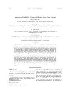
FIG. 1. Velocities at 08, 818E: (a) zonal and (c) meridional components of ADCP data (Reppin et al. 1999); (b) zonal and (d) meridional components of model data. Observations have been smoothed with a 3-day running mean filter to make them consistent with model data. Units are in m s 21 .
usual onset time of El Nin˜o (during boreal fall/early winter). This might explain why the subsequent model results show weaker amplitudes in the Pacific than in the Indian Ocean. 3. Comparison of model results with mooring data in the central equatorial Indian Ocean Figure 1 shows time series of ADCP data (Reppin et al. 1999) and simulated current components over a 14months-long mooring. A 3-day running mean filter has been applied to the observations to make them comparable with the model dataset. The observed zonal surface currents in Fig. 1a show two equatorial jets during late 1993 (October–December) and early 1994 (March– May). The Wyrtki jets during late 1993 reached maximum eastward surface speeds of more than 1.6 m s 21 . The model results (Fig. 1b) resemble the measurements at 808E during fall 1993 with peak zonal velocities of more than 1.2 m s 21 . However, the model overestimates the total spring eastward circulation at the surface. The strongest signal of the subsurface equatorial undercurrent (EUC) appeared in the observations in early 1994 with currents reaching 0.8 m s 21 at 95 m (red color in Fig. 1 denoting flow to east). The model generally un-
derestimates the eastward EUC and occasionally gets the sign wrong (weak westward circulation in the model at the level of the EUC in early 1994). Figures 1c,d show the corresponding meridional currents. Large variability on submonthly timescales and upward phase propagation for the deeper levels can be seen in both model results and observations. However, the simulated current amplitude is again smaller than observed. Part of the problem might be related to inaccurate surface forcing fields. Figures 2a,b show the surface wind fields at 08N, 818E from the blended FSU–NCEP wind product that has been used to force the model, as well as observations from a mooring at the same site (M. McPhaden 2000, personal communication). The zonal wind components show reasonable agreement, though unfortunately the mooring was removed in January 1994, so we cannot tell wether the overstrong surface current in March–May 1994 in Fig. 1b is due to winds or model problems. From July to early August 1993 and from October 1993 to December 1993 the meridional winds from mooring data and the blended FSU–NCEP winds frequently have opposite signs, and on short timescales the variability of the FSU–NCEP product is generally less than observed. Furthermore, simulated SST (Fig. 2d) is too warm by as much as 0.88C during the first
26
JOURNAL OF CLIMATE
VOLUME 16
on all timescales up to annual, despite discrepancies in observed wind products as well as in simulated and observed SST. We have attempted to use the data of Figs. 1 and 2 to further clarify the response of the ocean to boreal summer intraseasonal events. Unfortunately, only one of the 26 intraseasonal events used in the present study occurred while the ocean mooring was in place and no event occurred during the measurement phase of the meteorological buoy (for dates of these events see Table 2). There is wide variability among the intraseasonal events, and winds during that one event centered at 25 April 1994 were quite dissimilar to the composite winds discussed in the following sections. Therefore we have been unable to pursue this topic further. 4. Dynamics of intraseasonal SST modulation a. Atmospheric forcing and SST pattern
FIG. 2. Surface fields at 08, 818E for Jul 1993–Jan 1994: (a) zonal, (b) meridional surface winds (m s 21 ); (c) wind speeds (m s 21 ); (d) SST (8C); (e) time rate of change of SST (8C day 21 ). Solid lines are observations from a surface mooring (M. McPhaden 2000, personal communication). Dotted lines in (a)–(c) are blended NCEP–FSU winds; dashed lines in (d), (e) denote observed SST (Reynolds and Smith 1994) and dashed–dotted lines in (d), (e) are model data. Vertical lines in (a), (b) denote active (‘‘A’’) and break (‘‘B’’) periods of the monsoon as defined by Webster et al. (1998). Observational data have been smoothed with a 3-day running mean filter.
half of the record. Note, however, the differences between the two observational products. Even high-quality products like the Reynolds SST data can contain significant errors on intraseasonal timescales of more than 0.58C, as was shown by Premkumar et al. (2000) by comparing Reynolds data with buoy data in the Bay of Bengal. The time rate of change of SST in the model and in the Reynolds and Smith (1994) data (Fig. 2e) is much smaller than in the mooring data. The discrepancy between model and mooring data might by associated with the thick (15 m) uppermost level in our model. In reality, heat absorbed or released by the ocean might interact with a much thinner near-surface layer. Most of the large observed SST rises in Fig. 2d indeed occur at wind speeds less than about 4 m s 21 (Fig. 2c), indicating that the real mixed layer is less than 15 m deep (Weller and Anderson 1996). In summary, the model displays reasonable agreement with the available observations
Intraseasonal variations of precipitation and wind fields are associated with changes in the strength of the atmospheric monsoon circulation. Figure 3 shows anomaly composites of precipitation and 10-m winds. Organized convection occurs first in the western and central Indian Ocean (day 26). It intensifies and moves to the eastern Indian Ocean (day 0), before bifurcating northward and southward from the equator. At day zero, precipitation anomalies in the eastern equatorial Indian Ocean exceed 16 mm day 21 . A comparison of days 26 and 16 shows differences in the sign of the anomalous atmospheric circulation in the Arabian Sea and the equatorial western Indian Ocean; since these are boreal summer composites, they imply weaker (stronger) than normal monsoon winds on days 26 (16). The bifurcation of the equatorial precipitation anomalies after day 0 is accompanied by basin-scale troughs that migrate eastward, northward, and occasionally southward (Webster et al. 1998; Lawrence and Webster 2002). Associated positive precipitation anomalies at day 16 show a southeastward propagation that is associated with enhanced rainfall over southwest Australia. The large-scale signatures in wind fields and precipitation during intraseasonal events suggest accompanying changes in ocean circulation and heat budgets. Anomaly composites of simulated and observed SST (Reynolds and Smith 1994; Fig. 4) reveal a basinwide oceanic response to the atmospheric forcing pattern. During the initial calm and clear phase of an intraseasonal event, warm anomalies exist throughout the tropical Indian Ocean, whereas the Pacific Ocean is still influenced by the windy and cloudy phase of the previous event (days 212, 26). Strong westerly wind anomalies in the equatorial Indian Ocean at around days 0 to 16 (Fig. 3) lower the SST over the entire region. At the same time, conditions in the Pacific are sunny (as indicated by negative precipitation anomalies at day 0, Fig. 3b), and wind speeds are weak, so SST rises. At
1 JANUARY 2003
SCHILLER AND GODFREY
27
FIG. 3. Anomaly composites of MSU precipitation (NCEP reanalysis data outside 158N–S) and 10-m winds (NCEP blended with FSU data). Time is defined as maximum of precipitation at 908E (5day 0). Vector magnitude (m s 21 ) and precipitation rates (mm day 21 ) are shown at bottom. Note that precipitation anomalies in the eastern equatorial Indian Ocean exceed the scale used here (.16 mm day 21 ).
the end of this (half ) cycle SSTs in the whole equatorial Indian and western Pacific Oceans have changed sign (day 112). SST variations are associated with a waning (prior to the event) and waxing (after the event) of the entire monsoon gyre. Comparison of Figs. 3 and 4 reveals that warm SSTs in the Indian Ocean are associated with an anomalously weak southwest monsoon circulation, and the cooler SSTs are associated with an anomalously strong southwest monsoon. While the model slightly underestimates the extent of the large-scale SST anomaly pattern, regional extrema and associated phases are reasonably well reproduced. SST signals in the western Pacific are smaller in amplitude than in the Indian Ocean, which might be related to our definition of intraseasonal variability (which contains the complete set of subseasonal signals, including noise) and also to the restriction to boreal spring/summer intraseasonal events,
which might have a smaller amplitude in the Pacific than their boreal winter counterparts. Note that amplitudes of simulated and observed composite signals in the Indian Ocean are about 0.28C. Given errors in forcing fields and model physics, this result is encouraging. It proves that OGCMs are capable of realistically simulating intraseasonal variability. Figure 5 shows standard deviations of the composite SST variability seen in Fig. 4, for model and observation. The first thing to note is that for both model and observation the variabilities are at least as large as the anomaly composites themselves (Fig. 4). This has significant implications for the definition of a ‘‘typical’’ intraseasonal event, as will be discussed below. Furthermore, variability of intraseasonal oscillations in the model shows a strong maximum in the central equatorial Indian Ocean just south of India and another one south
28
JOURNAL OF CLIMATE
VOLUME 16
FIG. 4. Anomaly composites of SST of (a)–(e) model and (f )–(j) observations (Reynolds and Smith 1994). Units are in 8C.
of Java. Both of these features exist in the observations too, but are slightly shifted in space with broader maxima. Discrepancies between simulated and observed variability on intraseasonal timescales exist along the western coastline off Somalia and off eastern India. The two observed maxima off Somalia are likely to be associated with short-term variability of two prominent features of the Somali current that exist at about the same geographical location: the ‘‘great whirl’’ and the ‘‘southern gyre,’’ which reach their maximum strength in June/July (Schott and McCreary 2001). Since these features are not resolved with our coarse-resolution model, the model simulation only shows slightly enhanced variability in this area. The simulated maximum
in SST variability in the western Arabian Sea does not exist in the observations and might be an artifact of the model. b. Mixed layer heat budget In order to gain a better insight in the oceanic processes associated with intraseasonal SST variability, it is useful to explore the mixed layer variability and the associated heat balance. During boreal spring and summer the mixed layer is shallow between the equator and 108S (Fig. 6a). The Findlater jet along the Somali coast and in the Arabian Sea causes strong mixing and thus mixed layer depths are deep during the southwest mon-
1 JANUARY 2003
29
SCHILLER AND GODFREY
FIG. 5. Std dev of SST anomaly composites for (a) model and (b) observations (Reynolds and Smith 1994). Units are in 8C.
soon, at least outside the narrow region of coastal upwelling. Anomalies of mixed layer depth (Figs. 6b–e) are shallower during the warming phase of the intraseasonal event (calm and clear conditions) and deeper during the cooling phase (windy and cloudy conditions). Largest amplitudes of intraseasonal mixed layer variability are found in the central and eastern equatorial Indian Ocean (ø12 m). The heat budget for the mixed layer can be written as
1
2
]T ]h ]T Q0 2 Qpen 1 u · =T 1 w 2 5 , ]t ]t ]z r 0 cp h
(4)
where T is the mixed layer temperature, u · =T is the horizontal advection, w is the vertical velocity at the mixed layer base, h is the mixed layer depth, Q 0 is the surface net heat flux, Qpen is the penetrative component of solar shortwave radiation below the mixed layer, r 0 is water density, and c p is specific heat. Horizontal diffusion has been found to be at least two orders of mag-
30
JOURNAL OF CLIMATE
FIG. 6. (a) Mean composite mixed layer depth and (b)–(e) anomaly composites of mixed layer depth. Contour interval is (a) 25 m and (b)–(e) 2 m. Zero lines have been omitted.
nitudes smaller than any other term and has been omitted from Eq. (4). Due to the ambiguity in the definition of the vertical temperature gradient ]T/]z in the entrainment term (w 2 ]h/]t)]T/]z and because all other terms are readily available from the model output, we calculated the entrainment term as the residuum of Eq. (4). We also note that there is no well-defined mixed layer depth in the model (the ‘‘real mixed layer’’ consists of
VOLUME 16
the bulk component plus the Richardson number–dependent component, see section 2a), which prevents us from directly calculating the entrainment heat flux. The most important term in the mixed layer heat budget is the net surface heat flux minus the small penetrative component of solar shortwave radiation (Figs. 7a–e), shown here as time rate of change in mixed layer temperature. During the calm and clear phase of the intraseasonal event (days 212, 26) the tropical Indian Ocean gains heat and therefore surface heat fluxes contribute to the warming in SST (Fig. 4). Westerly wind anomalies at about day 0 cause equatorial cooling in the central Indian Ocean; the surface heat loss peaks at about 60 W m 22 in the eastern Indian Ocean. By day 112 of the intraseasonal oscillation, equatorial Indian Ocean winds have weakened and rainfall decreased, and the equatorial net heat flux becomes again weakly positive. The amplitude of the surface net heat flux accounts for typically about 75% of the composite change in SST. This dominance of the net surface heat flux on SST anomalies is confirmed by comparison of Figs. 4 and 7a–e, which reveal that SST anomalies lag the net surface heat flux by about 1/4 cycle (6–9 days), in close agreement with the theroretical value and the assumption of a constant mixed layer depth (Shinoda and Hendon 1998). It is interesting to note that composite surface flux anomalies in the western Bay of Bengal and the eastern Arabian Sea are out of phase with the equatorial component, similar to the precipitation anomalies shown in Fig. 3. The latter were first remarked upon by Gadgil et al. (1984), who noted that rain on the equator south of India was often anticorrelated with that over the Bay of Bengal, as if rain events at the two locations competed with one another. This seminal paper motivated many later studies of intraseasonal activity in the Indian Ocean. Using data from TRMM, recent research has confirmed this anticorrelation (Harrison and Vecchi 2001; Sengupta et al. 2001a). Despite the lack of coherent basin-scale signals and a distinct intraseasonal cycle, vertical entrainment does contribute to the mixed layer heat budget, as can be seen in Figs. 7f–j. Entrainment anomalies can be both positive and negative. Maxima of composite entrainment amplitudes are located in the western Bay of Bengal and in the central and eastern Indian Ocean for day 0. Alongshore wind anomalies (Fig. 3) favor coastal upwelling on intraseasonal timescales, in particular along the coastlines of Somalia and Sumatra/Java. In the central Indian Ocean a large area of entrainment warming just south of the equator can be associated with offequatorial upwelling at around day 0. Maximum values of entrainment warming reach 0.058C day 21 and are as large as the net surface heat flux, that is, with peaks at about 60 W m 22 . In most areas the temperature trend due to entrainment is seen to be out of phase with the temperature trend due to net surface heat flux, such that when the surface heat flux is most negative (e.g., at day 0 along the equator; Fig. 7c), entrainment warming acts
1 JANUARY 2003
SCHILLER AND GODFREY
31
FIG. 7. Anomaly composites in mixed layer: (a)–(e) temperature trend due to net surface heat flux minus penetrative component, and (f )–(j) due to entrainment at the base of the mixed layer. Units are in 8C day 21 .
to warm the mixed layer (Fig. 7h) and vice versa. Note that at day 0 entrainment warms, rather than cools the surface mixed layer. This surprising result is examined in more detail below. To understand the underlying physical mechanism that causes such anomalously warm entrainment fluxes an example is shown and discussed for the equator at 08, 818E, (Figs. 8a–c; we pay particular attention to the site at 08, 818E as it is close to the modeled and observed maxima in intraseasonal SST variability). Low winds, light mixing, and a positive shortwave flux into the ocean during the calm and clear phase of the intraseasonal event favor the development of a shallow mixed layer and allow part of the solar shortwave radiation to penetrate below the surface
mixed layer (26 June 1992 in Figs. 8a–c). As a result, a temperature inversion develops. The temperature inversions in the central and eastern equatorial Indian Ocean are accompanied by a shallow and permanent halocline, which result from long-term freshwater gains at the surface. The resulting mixed layer is shallower than the isothermal layer, the distance separating the top of the thermocline and the bottom of the mixed layer is referred to as the barrier layer. Temperature inversions and barrier layers are a frequent feature in the central and eastern Indian Ocean (Sprintall and Tomczak 1992). Godfrey et al. (1999) observed an example of such a temperature inversion and entrainment warming directly. With the onset of the cloudy and windy phase of the intraseasonal
32
JOURNAL OF CLIMATE
VOLUME 16
FIG. 8. Vertical profiles at 08, 818E of potential temperature, salinity, and density sQ for (a)– (c) Jun–Jul 1992 intraseasonal event and (d)–(f ) composites. Dates of profiles for an individual event and composites are shown in (c) and (f ). The peak of the intraseasonal event shown in (a)–(c) happened at 908E on 8 Jul 1992. The inlays in (a), (d) are enlargements of the corresponding temperature profiles in the top 90 m. Dotted lines in (d)–(f ) denote std dev for profiles at day 0.
oscillation (day 0) the mixed layer begins to lose heat through the surface, but enhanced vertical mixing entrains heat into the mixed layer, partly compensating the surface heat loss. For the individual event shown in Fig. 8a the temperature inversions persist throughout the whole event, whereas the composites in Fig. 8d indicate that warmer subsurface water is eventually completely entrained in the mixed layer and the mixed layer starts to deepen and to cool. As wind anomalies ease, surface heat flux anomalies become positive again and dominate the mixed layer heat budget, whereas entrainment fluxes vanish. Barrier-layer formation due to low surface salinity also happens in the composite profiles (Figs. 8d–f), but is smaller than for the individual event shown in the left column. Another interesting aspect of intraseasonal oscillations is their inherent variability among different events. We
have already pointed out in the discussion of Fig. 5 that intraseasonal composites in the Indian Ocean represent a mean signal with large standard deviations. This result is confirmed by inspection of composite standard deviations as shown in Figs. 8d–f, shown here on day 0 for temperature, salinity, and density. Standard deviations of these composited quantities are as large as or larger than the anomalies themselves. This result suggests that contributions from individual terms in the mixed layer heat budget may differ significantly from their composite ‘‘mean’’ values; that is, different processes may control intraseasonal dynamics in different events. Composite horizontal advection only plays a minor role in the mixed layer heat budget (not shown). While horizontal surface velocity anomalies reveal a distinct intraseasonal signal (Fig. 9e), horizontal temperature
1 JANUARY 2003
SCHILLER AND GODFREY
33
FIG. 9. Equatorial time–longitude sections of anomaly composites: (a) net surface heat flux [contour interval (c. i.) 5 10 W m 22 ], (b) solar shortwave radiation (c. i. 5 10 W m 22 ), (c) latent heat flux (c. i. 5 10 W m 22 ), (d) SST (c. i. 5 0.028C), (e) zonal sea surface velocity (c. i. 5 2 cm s 21 ), (f ) mixed layer depth (c. i. 5 2 m), (g) precipitation 2 evaporation (c. i. 5 1 mm day 21 ), (h) sea surface salinity (c. i. 5 0.02 psu). Zero lines have been omitted for clarity.
gradients at the mixed layer level are very small and thus minimize the impact of advection anomalies on the mixed layer temperature. Composite horizontal advection is typically one order of magnitude smaller than the heat flux term (,10 W m 22 , calculated as r 0 c p h times the horizontal advection anomaly). Furthermore, there is neither a clear temporal trend in the advection anomalies nor is there a basin-scale structure. In summary, net surface heat flux is the dominant term of the composite mixed layer heat budget on intraseasonal timescales, although entrainment of thermocline water contributes on a smaller spatial scale. To gain further insight into intraseasonal dynamics, Fig. 9 shows Hovmoeller plots of composites along the equatorial Indian and Pacific Oceans. Figures 9a–c reveal the dominance of solar shortwave radiation on the
surface net heat fluxes. A closer examination also shows that the maximum latent heat loss lags the minimum solar shortwave radiation (maximum convection) by about 2–3 days (not shown), consistent with previous analyses (e.g., Shinoda et al. 1998). Eastward propagation of solar shortwave radiation and SST anomalies happens at a speed of approximately 4–6 m s 21 , similar to the propagation speeds quoted for the MJO by other authors (e.g., Shinoda et al. 1998), but our intraseasonal signal probably contains additional intraseasonal frequencies. The equatorial surface net freshwater flux is dominated by the precipitation anomalies, as can be deduced from comparison of Figs. 9c and 9g: the maximum in latent heat flux corresponds to a maximum evaporation of about 1 mm day 21 , whereas precipitation accounts
34
JOURNAL OF CLIMATE
VOLUME 16
FIG. 11. Mean boreal spring–summer 1992 SST difference for model experiments with and without diurnal cycle in solar shortwave radiation. Contour interval is 0.18C. Shaded areas denote regions with 20.3 # DSST # 0.38C.
erally as large as the interannual signal, again indicating that individual intraseasonal events can create much stronger signals than revealed by their composites. The large variability in the composites is caused by variability in the forcing data, as indicated by the standard deviation of the zonal wind velocity at 10 m (Fig. 10a). FIG. 10. Anomaly composites at 08N, 818E: (a) zonal wind velocity at 10 m, (b) sea surface height, (c) mixed layer depth, (d) barrierlayer thickness, and (e) depth of 208 isotherm. Dashed lines are std dev.
for more than 10 mm day 21 in the far eastern equatorial Indian Ocean. Evaporation and precipitation are slightly shifted in phase, such that during the windy and cloudy phase precipitation excess leads evaporative cooling. Further details of the surface freshwater fluxes and the salinity budget will be discussed in section 5. Between 708 and 908E, the maximum in surface velocity (Fig. 9e) lags the surface winds (Fig. 3 and Fig. 10a) by about 6 days. Apart from this offset, the surface velocity mirrors the behavior of the surface winds. Thus one can see moisture divergence over Indonesia before the event (Fig. 3), changing to convergence at day 0, broadly compatible with Webster’s criterion used in this study for forming the intraseasonal composites (day 0 5 rainfall maximum at 908E). Changes in mixed layer depth (Figs. 9f, 10c), which is primarily controlled by surface fluxes, are accompanied by changes in variables that are mainly determined by three-dimensional ocean dynamics such as sea surface height (Fig. 10b) and depth of the 208 isotherm (Fig. 10e). The almost vanishing anomaly amplitude of the ‘‘deep’’ 208 isotherm suggests that intraseasonal variability is a surface-intensified process. Associated with strong variability in mixed layer depth (Figs. 9f, 10c), SST (Fig. 9d), and SSS (Fig. 9h) are fluctuations in barrier-layer thickness (Fig. 10d). While changes in all these variables are rather small compared to their interannual amplitudes, their standard deviations are gen-
c. Impact of the diurnal cycle Observations during the Tropical Ocean Global Atmosphere Coupled Ocean–Atmosphere Response Experiment (TOGA COARE; Weller and Anderson 1996) as well as modeling studies (Shinoda and Hendon 1998) provided evidence for the important impact of the diurnal cycle of solar shortwave radiation on SST. Furthermore, Shinoda and Hendon (1998) showed in two experiments that the diurnal cycle in solar insolation is responsible for a differential SST response, which is associated with the mean vertical distribution of heating during the day. The mixed layer is shallow during daytime, thus the heating is trapped near the surface and SST rapidly increases. During nighttime cooling deepens the mixed layer, but the cooling is distributed over a deeper layer (and in many cases involves mixing of temperature inversions that reduce the impact of the surface cooling). Hence, the SST with diurnal forcing is warmer and the submixed layer is cooler than would be the case with daily mean forcing. To verify these results with our model, we repeated one year of our experiment, but without a diurnal cycle in solar shortwave radiation. In the tropical Indian Ocean, we found similar results to Shinoda and Hendon (1998); that is, 3-day mean SSTs with diurnal cycle are persistently about 0.18–0.38C higher than without (Fig. 11). This good agreement is somewhat surprising, as we use a vertical resolution of 15 m in the upper ocean, which is much coarser than in previous work based on 1D mixed layer models (ø1 m). Note, however, that the change in SST is not homogeneous; in the Indonesian Archipelago and in the subtropical convergence zone of
1 JANUARY 2003
35
SCHILLER AND GODFREY
FIG. 12. Vertical profiles at 08N, 818E of potential temperature, salinity, density sQ for Jul–Aug 1992 intraseasonal event. Left (right) column shows profiles obtained with (without) simulated diurnal cycle in solar shortwave radiation. Inlays in (a), (d) are enlargements of the composite temperature profiles in the top 90 m. The peak of the intraseasonal event happened at 908E on 3 Aug 1992.
the South Pacific the diurnal cycle causes a slight cooling in SST. Furthermore, in areas of shallow mixed layer, like the northern Arabian Sea, the northern Bay of Bengal, and along coastlines the increase in SST due to diurnal forcing can exceed 18C. The impact of diurnal forcing on vertical property distributions is illustrated in Fig. 12. It shows vertical profiles of temperature, salinity, and densitity of an intraseasonal event in July–August 1992 at 08, 818E. The overall cooling trend in the 3-day mean temperature near the surface is clearly visible. Another feature is the indirect impact of the diurnal cycle on the salinity structure. The most striking differences between Figs. 12b and 12e is that salinity increases steadily over the 24 days in Fig. 12e, throughout the top 120 m; this is not apparent in Fig. 12b. Plots of horizontal velocities at this location (not shown) reveal
small differences between the two runs of the order of 10 cm s21 . As this is a region of strong salinity gradients (see section 5), these small velocity differences may be responsible for the differences between Figs. 12b and 12e. The salinity differences are also reflected in the vertical density profiles (Figs. 12c,f). 5. Intraseasonal sea surface salinity modulation Intraseasonal salinity fluctuations in the mixed layer influence the vertical density structure and therefore, indirectly, the mixed layer heat budget. The salinity budget for the mixed layer can be written as
1
2
]S ]h ]S 2(P 2 E )S 1 u · =S 1 w 2 5 , ]t ]t ]z h
(5)
36
JOURNAL OF CLIMATE
VOLUME 16
FIG. 14. Boreal spring-to-summer (AMJJAS) mean sea surface salinity. Contour interval is 0.2 psu. FIG. 13. Anomaly composites of mixed layer salinity budget at (a) 08N, 818E and (b) 08N, 948E: time-rate-of-change of mixed layer salinity (thick solid line), surface freshwater flux (evaporation minus precipitation, thin solid line), horizontal advection (dashed), meridional advection (dotted) and entrainment (dashed–dotted).
where S is the mixed layer salinity, and (P 2 E) is the surface freshwater flux [all other variables are defined in Eq. (4)]. Composites of surface freshwater fluxes and entrainment of salinity are very similar in their pattern to their heat budget counterparts in Fig. 7 (not shown). Negative freshwater fluxes prior and after the event tend to increase the mixed layer salinities and negative salinity trends due to strong precipitation during the event tend to reduce mixed layer salinities. Vertical entrainment acts the opposite way. However, in contrast to the heat budget, composite anomalies of sea surface salinity (and mixed layer salinity likewise) contain a less coherent large-scale structure than SST (Fig. 4). The reason for this different behavior becomes obvious in Fig. 13, which shows two examples of the composite mixed layer salinity budget for the central and eastern equatorial Indian Ocean. The consistent feature of the mixed layer salinity budget in the whole eastern basin is the lack of dominance of the freshwater fluxes over advection and entrainment. In the far eastern Indian Ocean (08, 948E; Fig. 13b) the horizontal advection terms are as important as the freshwater flux, despite strong precipitation at around day 0 there. The importance of advection in the salinity budget is associated with notable mean horizontal salinity gradients in this region (Fig. 14), but very weak SST gradients (the Indian Ocean part of the ‘‘warm pool’’). The strong horizontal sea surface salinity gradients are accompanied by strong intraseasonal zonal jets and somewhat weaker meridional anomalies (Fig. 15). The horizontal jets are tightly linked to the intraseasonal surface wind forcing (Fig. 3), but show a delay in their response by about 3–6 days. The mean equatorial surface circulation during boreal spring and summer (southwest monsoon) is eastward. Consequently, the development of the intraseasonal jets is associated with a delayed waning (prior and after the event) and waxing
(peak at around days 3–6 of an event) of the equatorial monsoon circulation. Ralph et al. (1997) and Shinoda and Hendon (2001) reported on similar intraseasonal jets in the equatorial western Pacific with absolute velocities of about 1 m s 21 ; the anomaly component of this jet can also be seen in our model. However, more importantly for this study is the fact that the intraseasonal equatorial jets are generated in the Indian Ocean too, which ultimately contribute to the strong advection signal in the surface salinity budget. 6. Conclusions Using an OGCM with 3-day-averaged surface forcing, we demonstrated that today’s OGCMs are capable of simulating the large-scale pattern of observed intraseasonal SST variability in the tropical Indian Ocean. Composites of 26 intraseasonal events have been investigated to explore details of intraseasonal mixed layer dynamics. Simulated and observed composite SST anomalies are as large as 0.28C (with individual events revealing amplitudes up to 18C). This result is encouraging, although recent results show that a new SST product based on the Tropical Rainfall Measuring Mission (TRMM) performs better on short timescales than the Reynolds data used for model verification in this study (Harrison and Vecchi 2001; Sengupta et al. 2001a). Net surface heat flux was found to be the dominant factor in mixed layer dynamics, although locally vertical entrainment through the base of the mixed layer can be as strong as net surface heat flux. Strong entrainment at the peak of an intraseasonal event rather warms than cools the surface due to a mean temperature inversion. In the Indian Ocean shortwave radiation is more important for driving SST variations than latent heat flux variations, consistent with the findings of Shinoda and Hendon (1998). Anomalous precipitation in association with solar shortwave penetration and low winds favor the development of an intraseasonal barrier layer and temperature inversions, similar to the results of Shinoda and Lukas (1995) and Vialard and Delecluse (1998). Despite our finding that composite horizontal advec-
1 JANUARY 2003
SCHILLER AND GODFREY
37
FIG. 15. Anomaly composites of (a) zonal and (b) meridional surface velocity components. Units are in m s 21 .
tion anomalies within the mixed layer appear to be of only secondary importance to intraseasonal variability in the mixed layer heat budget, when investigating data from TOGA COARE in the western equatorial Pacific, Cronin and McPhaden (1997) and Feng et al. (2000) found strong signals in horizontal advection on intraseasonal timescales. Shinoda and Hendon (1998) noted that their one-dimensional model (which does not include horizontal advection), when forced with data from
the IMET mooring, failed in the western Pacific during a period that appeared to be subject to strong horizontal advection. These results and our own findings imply that intraseasonal variability is predominantly a onedimensional process. However, in order to capture all dynamical components of this climate signal it is important to apply three-dimensional models. Shinoda and Hendon (1998) found that the opposite phases of entrainment heat flux and net surface heat flux
38
JOURNAL OF CLIMATE
are associated with the strong diurnal cycle in their model, such that during the warming phase of an intraseasonal event, nighttime deepening of the mixed layer entrains cold water into it. We found a similar phase shift between net surface heat flux and entrainment heat flux. This anticorrelation stems from the opposite impact wind anomalies cause in the presence of temperature inversions to surface heat flux and entrainment. During the clear and calm phase weak winds and strong insolation cause positive surface heat flux anomalies, which supports the buildup of a barrier layer and temperature inversions below the mixed layer. With the onset of the windy phase, entrainment becomes initially positive at around day 0, as the temperature inversion are entrained into the mixed layer. As the windy and cloudy phase continues, the surface starts to lose heat and further deepening of the mixed layer causes the entrainment flux to become negative. Finally, as winds ease, surface heat flux anomalies become positive again and entrainment heat fluxes disappear. Despite using a coarse vertical resolution in our model (15 m near the surface), we were able to confirm earlier results (Shinoda and Hendon 1998) that the diurnal cycle of solar shortwave radiation significantly increases the amplitude of SST over that produced by daily mean insolation. It is therefore important to resolve the diurnal cycle in coupled models that aim to simulate intraseasonal variability. In contrast to the mixed layer heat budget the salinity budget is about equally determined by surface freshwater fluxes, horizontal advection, and vertical entrainment. Horizontal advection of salinity is important in the central and eastern Indian Ocean because of the existence of notable zonal salinity gradients and jetlike intraseasonal surface current anomalies. Along the equator, the latter reaches anomalous currents of the order of 20 cm s 21 and is tightly coupled to intraseasonal atmospheric wind forcing (with a delay of 3–6 days). Kessler and Kleeman (2000) used an OGCM, forced with idealized, purely oscillating wind stresses to explore rectified SST anomalies caused by MJO–ENSO feedbacks. They found that MJOs can interact constructively with the ENSO cycle, such that MJO-like wind stresses cause changes in SST of opposite signs in the equatorial western and central Pacific. This effect tends to flatten the background zonal SST gradient and eventually leads to additional westerlies and stronger El Nin˜os. In this paper, we have explored intraseasonal variability forced by observation-based winds, and we have focused on the active phases of intraseasonal variability. Therefore, the interesting question, if a complete intraseasonal cycle in the Indian Ocean leaves behind a net change is SST, is beyond the scope of this paper. Dynamical seasonal prediction of the monsoon system is an ongoing global research effort. Unfortunately, accurate forecasting of the monsoon system and associated intraseasonal variability is still hampered by problems encountered with coupled models and has thus far
VOLUME 16
proven elusive (e.g., Slingo et al. 1999; Sperber et al. 2001). Acknowledgments. The authors would like to thank Peter Webster for providing us with information about individual dates of intraseasonal events. We also thank Fritz Schott and Mike McPhaden for sharing with us their hydrographic and meteorological datasets. Two anonymous reviewers provided helpful comments on improving the manuscript. Interpolated OLR data were provided by the NOAA–CIRES Climate Diagnostics Center, Boulder, Colorado, from their Web site online at http://www.cdc.noaa.gov/. Russell Fiedler and Jim Mansbridge prepared the forcing datasets and helped with the visualization. All plots have been created with the FERRET plot software package (http:// www.pmel.noaa.gov). This work is partly funded by Australia’s CSIRO and by a grant from the Land and Water Resources Research and Development Corporation. REFERENCES Chen, D., A. J. Busalacchi, and L. M. Rothstein, 1994a: The roles of vertical mixing, solar radiation, and wind stress in a model simulation of the sea surface temperature seasonal cycle in the tropical Pacific Ocean. J. Geophys. Res., 99, 20 345–20 359. ——, L. M. Rothstein, and A. J. Busalacchi, 1994b: A hybrid vertical mixing scheme and its application to tropical ocean models. J. Phys. Oceanogr., 24, 2156–2179. Cronin, M. F., and M. J. McPhaden, 1997: The upper ocean heat balance in the western equatorial Pacific warm pool during September–December 1992. J. Geophys. Res., 102, 8533–8553. Emanuel, K. A., 1987: An air–sea interaction model of intraseasonal oscillations in the tropics. J. Atmos. Sci., 44, 2324–2340. Feng, M., R. Lukas, P. Hacker, R. A. Weller, and S. P. Anderson, 2000: Upper-ocean heat and salt balances in the western equatorial Pacific in response to the intraseasonal oscillation during TOGA COARE. J. Climate, 13, 2409–2427. Gadgil, S., P. V. Joseph, and N. V. Joshi, 1984: Ocean–atmosphere coupling over monsoon regions. Nature, 312, 141–143. Godfrey, J. S., and A. Schiller, 1997: Tests of mixed layer schemes and surface boundary conditions in an ocean general circulation model, using an equatorial data set. CSIRO Rep. 231, 39 pp. ——, E. F. Bradley, P. A. Coppin, L. F. Pender, T. J. McDougall, E. W. Schulz, and I. Helmond, 1999: Measurements of upper ocean heat and freshwater budgets near a drifting buoy in the equatorial Indian Ocean. J. Geophys. Res., 104, 13 269–13 302. Harrison, D. E., and G. A. Vecchi, 2001: January 1999 Indian Ocean cooling event. Geophys. Res. Lett., 28, 317–3720. Hendon, H. H., 2000: Impact of air–sea coupling on the Madden– Julian oscillation in a general circulation model. J. Atmos. Sci., 57, 3939–3952. ——, and J. Glick, 1997: Intraseasonal air–sea interaction in the tropical Indian and Pacific Oceans. J. Climate, 10, 647–661. Jones, C., D. E. Waliser, and C. Gautier, 1998: The influence of the Madden–Julian oscillation on ocean surface heat fluxes and sea surface temperature. J. Climate, 11, 1057–1072. Kalnay, E., and Coauthors, 1996: The NCEP/NCAR 40-Year Reanalysis Project. Bull. Amer. Meteor. Soc., 77, 437–471. Kessler, W. S., and R. Kleeman, 2000: Rectification of the Madden– Julian oscillation into the ENSO cycle. J. Climate, 13, 3560– 3575. ——, M. J. McPhaden, and K. M. Weickmann, 1995: Forcing of
1 JANUARY 2003
SCHILLER AND GODFREY
intraseasonal Kelvin waves in the equatorial Pacific. J. Geophys. Res., 100, 10 613–10 631. Kleeman, R., and S. B. Power, 1995: A simple atmospheric model of surface heat flux for use in ocean modeling studies. J. Phys. Oceanogr., 25, 92–105. ——, B. J. McAvaney, and R. C. Balgovind, 1993: An analysis of the interannual heat flux response in an atmospheric general circulation model. J. Geophys. Res., 99D, 5539–5550. ——, R. A. Colman, N. R. Smith, and S. B. Power, 1996: A recent change in the mean state of the Pacific basin climate: Observational evidence and atmospheric and oceanic processes. J. Geophys. Res., 101, 20 483–20 499. Lau, K.-M., and C.-H. Sui, 1997: Mechanisms of short-term sea surface temperature regulation: Observations during TOGA COARE. J. Climate, 10, 465–472. Lawrence, D., and P. J. Webster, 2002: The boreal summer intraseasonal oscillation: Relationship between northward and eastward movement of convection. J. Atmos. Sci., 59, 1593–1606. Legler, D. M., I. M. Navon, and J. J. O’Brien, 1989: Objective analysis of pseudostress over the Indian Ocean using a direct-minimization approach. Mon. Wea. Rev., 117, 709–720. Levitus, S., R. Burgett, and T. Boyer, 1994: World Ocean Atlas 1994, Salinity. Vol. 3, NOAA Atlas NESDIS 3, 99 pp. Madden, R., and P. R. Julian, 1971: Detection of a 40–50 day oscillation in the zonal wind in the tropical Pacific. J. Atmos. Sci., 28, 802–708. Niiler, P. P., and E. B. Kraus, 1977: One-dimensional models of the upper ocean. Modeling and Prediction of the Upper Layers of the Ocean, E. B. Kraus, Ed., Pergamon, 143–172. Pacanowski, R. C., 1995: MOM2 documentation user’s guide and reference manual: Version 1.0. GFDL Tech. Rep. 3, 232 pp. ——, and S. G. H. Philander, 1981: Parameterization of vertical mixing in numerical models of tropical oceans. J. Phys. Oceanogr., 11, 1443–1451. Peters, H., M. C. Gregg, and J. M. Toole, 1988: On the parameterization of equatorial turbulence. J. Geophys. Res., 93, 1199– 1218. Power, S. B., R. Kleeman, R. A. Colman, and B. J. McAvaney, 1995: Modeling the surface heat flux response to long-lived SST anomalies in the North Atlantic. J. Climate, 8, 2161–2180. Premkumar, K., M. Ravichandran, S. R. Kalsi, D. Sengupta, and S. Gadgil, 2000: First results from a new observational system over the Indian seas. Curr. Sci., Indian Acad. Sci., 78, 323–330. Ralph, E. A., K. Bi, and P. P. Niiler, 1997: A Lagrangian description of the western equatorial Pacific response to the wind burst of December 1992. J. Climate, 10, 1706–1721. Rao, R. R., R. L. Molinari, and J. F. Fiesta, 1989: Evolution of climatological near-surface thermal structure of the tropical Indian Ocean. 1. Description of mean monthly mixed layer depth, and sea surface temperature, surface currents and surface meteorological fields. J. Geophys. Res., 94, 10 801–10 815. Reppin, J., F. A. Schott, and J. Fischer, 1999: Equatorial currents and transports in the upper central Indian Ocean: Annual cycle and interannual variability. J. Geophys. Res., 104, 15 495–15 514. Reynolds, R. W., and T. M. Smith, 1994: Improved global sea surface
39
temperature analyses using optimum interpolation. J. Climate, 7, 929–948. Schiller, A., 1999: How well does a coarse resolution circulation model simulate observed interannual variability in the upper Indian Ocean? Geophys. Res. Lett., 26, 1485–1488. Schott, F., and J. P. McCreary, 2001: The monsoon circulation of the Indian Ocean. Progress in Oceanography, Vol. 51, Pergamon, 1–123. Sengupta, D., B. N. Goswami, and R. Senan, 2001a: Coherent intraseasonal oscillations of ocean and atmosphere during the Asian summer monsoon. Geophys. Res. Lett., 28, 4127–4130. ——, R. Senan, and B. N. Goswami, 2001b: Origin of intraseasonal variability of circulation in the tropical central Indian Ocean. Geophys. Res. Lett., 28, 1267–1270. Shinoda, T., and R. Lukas, 1995: Lagrangian mixed layer modelling of the western equatorial Pacific. J. Geophys. Res., 100, 2523– 2541. ——, and H. H. Hendon, 1998: Mixed layer modeling of intraseasonal variability in the tropical western Pacific and Indian Oceans. J. Climate, 11, 2668–2685. ——, and ——, 2001: Upper-ocean heat budget in response to the Madden–Julian oscillation in the western equatorial Pacific. J. Climate, 14, 4147–4165. ——, ——, and J. Glick, 1998: Intraseasonal variability of surface fluxes and sea surface temperature in the tropical western Pacific and Indian Oceans. J. Climate, 11, 1685–1702. Slingo, J. M., D. P. Rowell, K. R. Sperber, and F. Nortley, 1999: On the predictability of the interannual behaviour of the Madden– Julian oscillation and its relationship to El Nin˜o. Quart. J. Roy. Meteor. Soc., 125, 583–609. Sperber, K.R., and Coauthors, 2001: Dynamical seasonal predictability of the Asian summer monsoon. Mon. Wea. Rev., 129, 2226–2248. Sprintall, J., and M. Tomczak, 1992: Evidence of the barrier layer in the surface layer of the tropics. J. Geophys. Res., 97, 7305–7316. Stricherz, J., J. O’Brien, and D. Legler, 1992: Atlas of Florida State University Tropical Pacific Winds for TOGA 1966–1985. Florida State University, 256 pp. Vialard, J., and P. Delecluse, 1998: An OGCM study for the TOGA decade. Part II: Barrier-layer formation and variability. J. Phys. Oceanogr., 28, 1089–1106. Waliser, D. E., K.-M. Lau, and J. H. Kim, 1999: The influence of coupled sea surface temperatures on the Madden–Julian oscillation: A model perturbation experiment. J. Atmos. Sci., 56, 333– 358. Webster, P. J., 2002: JASMINE: The scientific basis. Bull. Amer. Meteor. Soc., 83, 1603–1630. ——, V. O. Magana, T. N. Palmer, J. Shukla, R. A. Thomas, M. Yanai, and T. Yasunari, 1998: Monsoons: Processes, predictability, and the prospects for prediction. J. Geophys. Res., 103, 14 451–14 510. Weller, R. A., and S. P. Anderson, 1996: Surface meteorology and air–sea fluxes in the western equatorial Pacific warm pool during the TOGA coupled ocean–atmosphere response experiment. J. Climate, 9, 1959–1990. Wilson, S. G., 2000: How ocean vertical mixing and accumulation of warm surface water influence the ‘‘sharpness’’ of the equatorial thermocline. J. Climate, 13, 3638–3656.