Oct 6, 2018 - stability (i.e., âin the coreâ from a coalitional game theoretic perspective), and no ... Another solution that has received considerable attention ...... [22] M. J. Osborne and A. Rubinstein, A Course in Game Theory. MIT. Press ...
1
Indirect Mechanism Design for Efficient and Stable Renewable Energy Aggregation
arXiv:1810.02930v1 [cs.GT] 6 Oct 2018
Hossein Khazaei, Student Member, IEEE, and Yue Zhao, Member, IEEE
Abstract—Mechanism design is studied for aggregating renewable power producers (RPPs) in a two-settlement power market. Employing an indirect mechanism design framework, a payoff allocation mechanism (PAM) is derived from the competitive equilibrium (CE) of a specially formulated market with transferrable payoff. Given the designed mechanism, the strategic behaviors of the participating RPPs entail a non-cooperative game: It is proven that a unique pure Nash equilibrium (NE) exists among the RPPs, for which a closed-form expression is found. Moreover, it is proven that the designed mechanism achieves a number of key desirable properties at the NE: these include efficiency (i.e., an ideal “Price of Anarchy” of one), stability (i.e., “in the core” from a coalitional game theoretic perspective), and no collusion. In addition, it is shown that a set of desirable “ex-post” properties are also achieved by the designed mechanism. Extensive simulations are conducted and corroborate the theoretical results. Index Terms—Cost allocation, Nash equilibrium, mechanism design, coalitional game, renewable energy, electricity market
I. I NTRODUCTION Renewable energies play a central role in achieving a sustainable energy future. However, renewable energies such as wind and solar power are inherently non-dispatchable, and yet highly uncertain and variable. As a result, integrating renewable energies into power systems to serve loads raises significant reliability and efficiency challenges [1], [2]. A variety of approaches have been proposed to compensate for the uncertainty of renewable energies, such as improving renewable power generation forecast [2], employing better generation dispatch methods [3], energy storage deployment and control [4], [5], [6], and demand response programs [7], [8], [9]. Another solution that has received considerable attention is to aggregate statistically diverse renewable energy sources [1], [10], [11]. In an aggregation, renewable power producers (RPPs) pool their generation together so as to reduce the aggregate uncertainty and risk, and hence the corresponding cost of compensation for their uncertainties. Accordingly, by forming an aggregation, RPPs can in total earn a higher payoff. A key question in aggregating RPPs is thus how to allocate the total payoff of an aggregation among its member RPPs. Notably, aggregating renewable energies has been studied extensively in the context of a two-settlement power market model, consisting of a forward power market and a real time one. As such, RPPs participate in these markets in the same way as conventional generators do. With this model, allocating payoffs in an aggregation of RPPs has been studied in a coalitional game framework based on the joint probability H. Khazaei and Y. Zhao are with the Dept. of Electrical and Computer Engineering, Stony Brook University, Stony Brook, NY, 11794 USA (e-mails: {hossein.khazaei, yue.zhao.2}@stonybrook.edu).
distribution of all the RPPs’ uncertain generation [10], [11]. The primary interest in this setting is to find a payoff allocation solution that is stable/in the core of the game. This is in general computationally hard in the sense that the number of constraints of the corresponding optimization problem grows exponentially with the number of RPPs. To this end, the core is proven to be non-empty in [10], and a closed-form solution of a payoff allocation in the core is found in [11]. While this line of works achieve efficiency (with an optimal forward contract) and stability (with a payoff allocation in the core) in aggregating RPPs, an underlying assumption is that the aggregator knows the joint probability distribution of the RPPs’ generation. In practice, however, an aggregator typically does not have the best or full knowledge of such information about the RPPs: not only the amount of relevant information can be overwhelming to glean, but also the RPPs themselves often have better information privately about their own generation than the aggregator does. As a result, to aggregate renewables in practice, it is essential to consider an information collection step by the aggregator with the RPPs. Consequently, with this step, aggregating renewable energies in a two-settlement market constitutes a mechanism design problem (as will be shown in details in Section II-C). In short, the primary goal of such mechanism design is the following: Granted that all the RPPs behave strategically for their own interests under this mechanism, the aggregation can still achieve the same desirable outcome as if all the RPPs’ information are indeed known to the aggregator. In general, there’s complete freedom in designing the information collection step of the mechanism. In particular, when the aggregator does not elicit all available information from the RPPs, the mechanism is called an “indirect” one , (in contrast to a “direct” one when all information from the RPPs are requested by the aggregator upfront) [12]. Indeed, we would like an aggregator to elicit as little information as possible from the RPPs, while still guaranteeing the performance of the overall mechanism. To this end, a simple interface between aggregator and RPPs has been proposed in [13]: each RPP submits just a single number to the aggregator, and the aggregator simply passes on the sum of these numbers as the forward power contract for the entire aggregation. Based on this simple interface, the central design task is again on the payoff allocation among the RPPs, for which a number of payoff allocation mechanisms (PAMs) have been proposed [13], [14], [15], [16], [17], [18]. Under any given PAM, the RPPs’ strategic decision making entails a non-cooperative game (as will be described later in Section II-E), and properties of the Nash Equilibria of this game have been studied in [13], [14], [15], [16]. The existing PAMs in the literature, however, have only gained limited success, as some essential
and highly desired properties still cannot be achieved. In particular, achieving efficiency and stability/in the core at the Nash Equilibria remains to be an open question. Lastly, we note that mechanism design methods have also been employed in power markets for problems other than renewable energy aggregation, e.g., for incentivizing conventional generators to reveal truthful information [19]. In this paper, we investigate indirect mechanism design under the framework of the above simple interface. We propose a new payoff allocation mechanism, and show that all the essential desirable properties are achieved by this PAM. We first show that, given the designed mechanism, the outcome of the mechanism can be predicted by a unique Nash equilibrium (NE) among the RPPs, for which we provide a closed-form expression. Moreover, this unique NE is efficient, meaning that it achieves the maximum total payoff as if all information are known a-priori to the aggregator. Next, we show that, the proposed payoff allocation is stable/in the core at this unique NE, meaning that no subset of the RPPs have any incentive to leave the aggregation as they cannot possibly earn a higher payoff on their own. Furthermore, we show that the designed mechanism guarantees no collusion among the RPPs at the unique NE, as they cannot earn a higher payoff by colluding. Lastly, we show that a set of ex-post properties are achieved by the proposed mechanism (with results reported in part in [17]). We note that similar ex-post results have also been independently developed in a recent work [18]. The remainder of the paper is organized as follows. The problem is formulated in Section II, and the indirect mechanism design framework for aggregating RPPs is introduced. The design goals, i.e., the desired properties of the PAM are described in Section III. The main results are presented in Section IV, in which we show that the proposed PAM achieves all the desired properties. Analysis and proofs of the main results are provided in Section V. Another set of properties achieved in an “ex-post” sense by the proposed PAM are presented in Section VI. Simulations are conducted in Section VII. Conclusions are drawn in Section VIII. II. P ROBLEM F ORMULATION A. System Model We consider RPPs participating in a two-settlement power market consisting of a day-ahead (DA) and a real time (RT) market. As a baseline case, we first consider an RPP i who participates in the market separately from the other RPPs. In the DA market, RPP i’s generation at the time of interest in the next day is modeled as a random variable, denoted by Xi . (We assume that the joint probability density function for the vector of random variables X1 , . . . , XN exists.) RPP i then determines a forward power supply contract in the amount of ci to sell in the DA-market. Interchangabely, ci is also termed a day-ahead commitment. RPP i gets a payoff of pf ci where pf denotes the price in the DA market. At the delivery time in the next day, RPP i obtains its realized generation xi : a) If it faces a shortfall, i.e., ci −xi > 0, it needs to purchase the remaining power from the RT market at a real-time buying price pr,b , b) if it has excess power, i.e. xi −ci > 0, it can sell it in the RT-market at a real-time selling
price pr,s . In case excess power needs to be penalized as opposed to rewarded, we model such cases by having pr,s < 0. We make the assumption that pr,s ≤ pr,b , which must hold for no arbitrage. Intuitively, the higher uncertainty an RPP’s generation has at DA, the more cost it incurs to the RPP. Specifically, the realized payoff of an RPP i who separately participates in the market is given by Pisep , pf ci − pr,b (ci − xi )+ + pr,s (xi − ci )+
(1)
where (·)+ , max(0, ·)1 . We denote the expected payoff of RPP i at the time when ci is determined one day ahead by πisep (ci ) , E[Pisep ],
(2)
where the expectation is taken over the random generation Xi . Remark 1 (Model Assumptions on Prices): In this paper, we consider a price taking environment for the RPPs in the DA market, and thus the price pf is given. We also consider that some fixed values for the RT buying and selling prices pr,b and pr,s are assumed at DA. These values can be interpreted as the RPPs’ expectations of the RT prices if they were to experience a shortfall or a surplus, respectively. We note that the price taking assumption is a simplifying one, which assumes that none of the RPPs can affect the price significantly at DA due to its relatively small size. This provides a first order approximation of the problem that allows us to perform effective analysis and gain insight. The results will lay the foundation for further investigation of more general scenarios. In particular, we would like to note that our latest result following this paper has achieved some success in relaxing these assumptions, and has addressed the pricemaking scenarios in both DA and RT markets [20]. B. Aggregating Renewable Energies We consider an aggregator that aggregates the power generation from a set of N RPPs, denoted by N , and participates in the DA-RT market on behalf of the RPPs. Intuitively, aggregation reduces the total uncertainty for the RPPs due to the statistical compensation among the random power generation at DA, and hence brings economic benefit to them. In this paper, transmission network constraints are not considered, and are left for future work. In general, the aggregator takes actions in the DA and RT markets as follows: a. In the DA market, the aggregator determines an amount of forward power contract to sell, denoted by cN . b. At the delivery time, the aggregator collects all the realized generation from the RPPs, denoted by xN = P i∈N xi , to meet the commitment cN . The deviation is settled in the RT market in the same way as in Section II-A. The realized payoff of the aggregator is thus PN , pf cN − pr,b(cN − xN )+ + pr,s(xN −cN )+
(3)
Next, the aggregator returns a payoff Pi to each RPP i. 1 We
use the symbol , to define notations.
Remark 2 (Budget Balance): In this paper, we require the aggregator’s budget balance be satisfied in all circumstances: N X
Pi = PN .
generality of this design problem, as there is complete freedom in choosing what information to request from the RPPs, how they are used to determine cN , and how payoffs are allocated.
(4)
i=1
We note that this is a stronger condition than just requiring budget balance be satisfied in expectation. Accordingly, there are two decisions an aggregator needs to make: a) the total commitment cN at DA, and b) the set of payoff allocations {Pi } at RT. In making these decisions, two fundamental goals an aggregator would like to achieve are: • Efficiency: The total expected payoff of the aggregation πN = E[PN ] is maximized. • Fairness / Stability: The payoff allocation within the aggregation {Pi } are fair to each RPP. In this paper, we interpret fairness using the notion of stability/in the core from a coalitional game perspective, as will be described in detail in Section III. In particular, a) achieving efficiency depends on the aggregator’s decision on the total DA commitment cN , and b) with the optimal cN , achieving stability depends on the decisions on the RT payoff allocation {Pi }. The Ideal Case of Aggregator Having Full Information: To achieve efficiency and stability, making decisions on cN and {Pi } requires the aggregator to know sufficient information from the RPPs. The ideal case would be an aggregator with full information from the RPPs, in particular, the DA joint probability distribution of all the random generation {Xi }. Based on the joint probability distribution of {Xi }, closedform solutions of cN and {Pi } that achieve efficiency and stability have been found in [11], and will be used for numerical comparisons later. C. The Mechanism Design Problem In practice, however, it is unlikely for an aggregator to precisely know the DA joint probability distribution of {Xi } for a number of reasons: a) the best information on future power generation may only be privately known to the RPPs, and b) the amount of information can be overwhelmingly large and difficult to glean for a single aggregator, especially when the number of RPPs becomes large, (consider, e.g., hundreds of thousands of distributed energy resources in a power distribution system). In this paper, we do not assume the aggregator knows any information a-priori at DA on the RPPs’ random generation {Xi }. Instead, we consider a general framework in which the aggregator elicits information from the RPPs, based on which decisions on cN and {Pi } are then made. As such, the aggregator’s actions involve the following three general steps: a. Information Collection: At DA, the aggregator elicits certain information from the RPPs. b. Commitment: At DA, the aggregator determines a total DA commitment cN . c. Payoff Allocation: At RT, the aggregator allocates a payoff Pi to RPP i, i = 1, . . . , N . Specifying how these three steps are performed constitutes a mechanism design problem. It is important to note the
D. An Indirect Mechanism Design Framework In this mechanism design problem, it is not imperative for the aggregator to elicit all information from the RPPs. When the aggregator does elicit all information upfront, such a mechanism is called a “direct mechanism”; Otherwise, it is called an “indirect mechanism” [12]. Rather than restricting ourselves to direct mechanisms, more generally, we will investigate indirect mechanism design: We would like to elicit as little information from the RPPs as possible, while still guaranteeing efficiency and stability of the aggregation. In particular, we will investigate the following framework of indirect mechanisms employing a simple design of Steps a. (Information Collection) and b. (Commitment) [13]. a. At DA, the aggregator elicits a single number ci from each RPP i. PN b. At DA, the aggregator commits cN = i=1 ci . c. At RT, the aggregator allocates a payoff Pi to RPP i, i = 1, . . . , N . We term the number ci submitted by RPP i its DA commitment. Accordingly, the aggregator simply passes on the sum of the RPPs’ DA commitments as the aggregate commitment. As Steps a. and b. are now fully specified, the central design task is Step c. – Payoff Allocation. As such, the design and analysis of Payoff Allocation Mechanisms (PAMs) that determines Pi would be the focus of the remainder of the paper. E. Mechanism’s Outcome in a Non-Cooperative Game of Strategic RPPs Given any PAM that specifies the rule of determining Pi , a key question is how one predicts the outcome under this mechanism. To answer this question, we must understand the behavior of the RPPs given any mechanism. As an RPP i is free to submit any DA commitment ci to the aggregator, a rational and strategic RPP i would submit a ci at DA that maximizes its expected allocated payoff E[Pi ]. It is important to note that, given a PAM, E[Pi ] can also depend on the other RPPs’ submissions of commitments. Accordingly, we denote the expected payoff of RPP i by πi (ci , {c−i }) , E[Pi ],
(5)
where {c−i } denotes the set of the commitments of the RPPs other than i. Note that πi (ci , {c−i }) depends on the particular design of the PAM. Therefore, the strategic decision making of the N RPPs on their submissions {ci } at DA can be studied under a noncooperative game framework, (termed a “contract game” in [13].) To predict the outcome of any designed mechanism, a natural solution concept is the Nash equilibria of this non-cooperative game2 . Specifically, given a PAM, a set of 2 We note that, in practice, NE may not be achieved in a dynamic market. Investigation of other solution concepts is left for future work.
commitments {cne i } is at a pure Nash equilibrium (NE) if they satisfy � ne � cne , ∀i. (6) i ∈ argmax πi ci , c−i ci
As such, an NE offers a stable3 outcome of the RPPs’ decision making on their commitments, as no RPP has any incentive to deviate from its already best responding commitment. In the remainder of the paper, we devote the notation {cne i } to denoting a set of commitments at a pure NE. As a mechanism designer for aggregating RPPs, we are interested in designing a PAM so that a set of essential and desirable properties can be achieved at equilibria of this noncooperative game, given the designed PAM.
i∈T
III. D ESIGN G OALS : D ESIRED E FFICIENCY AND S TABILITY P ROPERTIES
where
In this section, we provide a detailed description of the desired properties in designing PAM for aggregating RPPs. 1) Existence and uniqueness of pure Nash equilibrium: For a mechanism to have predictable outcomes, it is desired that the non-cooperative game among the RPPs induced by the mechanism has a unique pure NE, which would be the unique outcome that one shall predict from the RPPs’ strategic decision making. 2) Efficient computation of NE: In particular, we are interested in whether the unique pure NE, if exists, can be computed in closed form. 3) Efficiency: A PAM is efficient if, at the NE, the aggregation achieves the maximum expected payoff for the entire of RPPs. Specifically, this means that PNgroup ne , cne c is equal to the optimal commitment for N i=1 i the entire aggregation c?N , argmax E[PN ]
(7)
cN
(cf. (3)). This optimal commitment can in fact be computed as a solution to a news-vendor problem (for which we refer readers to [21] for more details): � � f the p −pr,s −1 , where FN (xN ) is the cumulac?N = FN pr,b −pr,s tive distribution function PN (cdf) of the aggregate random generation XN = i=1 Xi . In this paper, we assume −1 that the inverse function FN (·) exists. 4) Individual rationality: At the NE, the expected payoff of RPP i should be at least as high as the maximum payoff it could have gotten had it separately participated in the DA-RT market. Specifically, � � ne � ∀i ∈ N , πi cne ≥ πisep c?,sep , (8) i , c−i i where c?,sep , argmax πisep (ci ) i
individual rationality satisfied (8), not a single RPP has any incentive to leave the aggregation. 5) Stability / In the core: A generalization of individual rationality to a much stronger sense of stability is being “in the core”, a property celebrated in coalitional game theory [22]. Specifically, being in the core means that the RPPs’ expected payoffs satisfy the following condition: if any subset T of the RPPs leave the aggregation, separately form their own aggregation, and then participate inPthe market based on their aggregate generation XT , i∈T Xi , their highest possible expected payoff would be no higher than the sum of their expected payoffs originally from the PAM at the NE. Specifically, X � � sep ne ∀T ⊂ N , πi cne c?,sep , (10) i , {c−i } ≥ πT T
(9)
ci
(cf. (1) and (2)). It is important to note that, the (separately) optimal commitment c?,sep is in general i not equal to the equilibrium commitment cne i . With 3 This notion of stability from NE is not the coalitional game theoretic stability which will be described as Property 5) in the next section.
� πTsep (cT ) , E pf cT − pr,b (cT − XT )+ � + pr,s (XT − cT )+ ,
(11)
and c?,sep , argmaxcT πTsep (cT ). As such, being in T the core means that, not only every single RPP, but all subsets of RPPs do not have any incentive to leave the aggregation. This implies a very strong sense of stability of an aggregation. 6) No collusion: Suppose a subset of RPPs join together as a single player before participating in the aggregation with the remaining RPPs. For now, we assume the remaining RPPs know the joining of these RPPs as a single player. Later, we will show that the DA commitments of the remaining RPPs at the NE actually do not depend on whether or not they know there is a collusion. Because of the change of the set of players, a new game, and hence new NE would arise. The expected payoff of this “joint player” at the new NE should be no higher than the sum of these RPPs’ expected payoffs at the NE of the original game. Otherwise, some RPPs could have incentives to collude, join together, and collectively interface with the aggregator as a single (and larger) RPP in order to earn a higher total payoff. Rigorously, no collusion is defined as follows: ∀T ⊆ N , X � ne � � ne � πi cne ≥π ˜T c˜ne ˜−T , (12) i , c−i T , c i∈T
� � ne where c˜ne ˜−T is the new NE of the new nonT , c cooperative game for the case when the RPPs in T join as a single player. IV. M AIN R ESULTS We now present the main results of this paper: a proposed payoff allocation mechanism, and how it achieves all the above desired properties 1) - 6). First, we propose the following payoff allocation mechanism: f r,b if xN − cN < 0 p ci + p (xi − ci ) Pi = pf ci + p∗ (xi − ci ) if xN − cN = 0 , (13) pf c + pr,s (x − c ) if xN − cN > 0 i i i
where pr,s ≤ p∗ ≤ pr,b , and p∗ can be chosen arbitrarily within this range. Remark 3 (Non-Concavity of the Non-Cooperative Game): Given the proposed PAM (13), it is worth noting that πi (ci , {c−i }) is not a concave function in ci . Thus, the non-cooperative game of DA commitments among the RPPs is not a concave game. As such, the behavior of the game (e.g., whether an NE exists) cannot be predicted from existing theories of concave games [23]. Nonetheless, we analyzed the game with new techniques, and the main results are described next. Due to the non-concavity of the non-cooperative game among the RPPs, the existence of a pure NE is not always guaranteed. In the following, we first show the closed form of the unique pure NE if any pure NE exists at all, and then show a necessary and sufficient condition for a pure NE to always exist regardless of the DA and RT prices. Theorem 1: Employing the PAM (13), if the noncooperative game among the RPPs (cf. Section II-E) possesses any pure NE, it must be unique, and is given by the following DA commitments: ∀i = 1, . . . , N , h i ? cne = E X = c (14) X i N i N , PN ? where� XN =� , argmaxcN E[PN ] = i=1 Xi , cN f r,s p −p −1 FN pr,b −pr,s , and FN (xN ) is the cdf of XN . Remark 4: To compute its equilibrium commitment, an RPP needs only to know the bivariate probability distribution function (pdf) of its own generation and the total generation of the aggregation, i.e., fXi XN (xi , xN ). As such, knowledge of the complete joint pdf of all the RPPs is not needed. Theorem 2: The non-cooperative game among the RPPs always possesses a pure NE if the following condition holds, dEXi |XN [Xi |XN = α] ≤ 1. (15) dα Conversely, if the condition (15) does not hold, then there exists a set of DA and RT prices such that a pure NE does not exist. Remark 5: We argue that the condition (15) is a reasonable one, as it holds when no single RPP “dominates” the entire aggregation. Consider the case when ∀i ∈ N , ∀α,
dEXk |XN [Xk |XN = α] > 1. (16) dα P [Xk |XN ] + i6=k EXi |XN [Xi |XN ] = XN ,
∃k ∈ N , α, s.t.,
Because EXk |XN we have that dEXk |XN [Xk |XN = α] dEX−k |XN [X−k |XN = α] + = 1, dα dα (17) P where X−k , i6=k Xi . From (16) and (17), we have dEX−k |XN [X−k |XN = α] < 0. (18) dα This means that the aggregation of all the RPPs other than k is negatively correlated with the entire aggregation. Intuitively speaking, this means that the single RPP k is not only negatively correlated with the aggregation of all the other RPPs, but also dominates them, and hence dominates the entire
aggregation. However, this is an unlikely situation especially when the number of RPPs is relatively large, and no single RPP can dominate the entire aggregation. For the rest of this paper, we assume that the condition (15) holds, and thus the unique pure NE of the game is given by (14) as in Theorem 1. The closed form of this pure NE immediately implies the following: Corollary 1: Given the PAM (13), efficiency of the aggregation is achieved at the unique pure NE, i.e., ? cne N = cN ,
(19)
PN
ne where cne N , i=1 ci . In other words, Corollary 1 implies that the designed mechanism achieves an ideal “Price of Anarchy” of one [12]. Furthermore, we have that all the remaining desired properties introduced in Section III are also achieved: Theorem 3: Employing the PAM (13), individual rationality, stability / in the core, and no collusion are achieved at the unique pure NE specified in (14). As a result of Theorems 1, 2, 3 and Corollary 1, we conclude that the proposed PAM (13) induces a unique NE among the RPPs, expressed in closed form (14), which is both efficient and stable (i.e., in the core from a coalitional game perspective) for the entire aggregation, and guarantees no collusion. We further note that, interestingly, results and techniques similar to our findings have independently been developed for an energy storage sharing problem in the recent works [24] and [25]. Lastly, while the proposed PAM (13) is shown to achieve all the desired properties, an interesting question is how its specific form is discovered. For this, we refer the readers to Appendix D, in which we show the PAM (13) can be derived from a competitive equilibrium of a specially formulated market with transferrable payoff [22].
V. A NALYSIS AND P ROOFS OF THE M AIN R ESULTS A. Understanding the Proposed PAM 1) The Excess Payoff from Aggregation: We first examine the excess payoff from aggregating the RPPs given a set of DA commitments {ci }, i.e., the difference between a) the realized payoff of the aggregation, and b) the sum of the realized payoffs of the RPPs had they separately participated in the DA-RT market using the same DA commitments {ci }. We define the following notations for the (realization dependent) sets of RPPs with generation surpluses and shortfalls: S + , {i ∈ N | xi − ci ≥ 0} , S − , {i ∈ N | xi − ci < 0} X X X X cS + , ci , xS + , xi , cS − , ci , xS − , xi . i∈S +
i∈S +
i∈S −
i∈S −
For convenience, we define c∅ = x∅ = 0. We then have the following lemma on expressing the excess payoff in terms of the above notations, whose proof is relegated to Appendix A. Lemma 1: The excess payoff from aggregating the RPPs is X sep PN − Pi i∈N
� = pr,b − pr,s min ((xS + − cS + ) , (cS − − xS − )) (20)
Lemma 1 implies that the excess payoff from aggregation is always non-negative. The excess payoff is zero if the RPPs either all have excesses or all have shortfalls, i.e., no compensation happens among the RPPs. 2) Intuition of the Proposed PAM: To understand the proposed PAM (13), let us consider the following two cases: • Case 1: The aggregation has a shortfall in total, i.e. xN − cN < 0. In this case, Pi = Pisep , ∀i ∈ S − , i.e., those RPPs with a shortfall earns exactly the same as if they each participates in the market separately. In comparison, ∀i ∈ S + , Pi − Pisep = (pr,b − pr,s )(xi − ci ). As a result, only those RPPs in S + can gain extra earnings compared to if they participate in the markets separately. In other words, when the aggregation has a shortfall, all the excess payoff (20) are allocated to those RPPs with a surplus. • Case 2: The aggregation has a surplus in total, i.e. xN − cN > 0. In this case, Pi = Pisep , ∀i ∈ S + , i.e., those RPPs with a surplus earn exactly the same as if they participate in the market separately. In comparison, ∀i ∈ S − , Pi − Pisep = (pr,b − pr,s )(ci − xi ). As a result, when the aggregation has a surplus, all the excess payoff (20) are allocated to those RPPs with a shortfall. While this may seem unintuitive at first glance, it can be understood as only rewarding those RPPs who “reduce the total deviation”, even when the total deviation is a surplus and reducing it means having a shortfall. Remark 6 (Marginal Profit): The proposed PAM (13) can also be understood as follows: At RT, given the total (possibly negative) extra generation xN − cN from the aggregation of RPPs, if an additional infinitesimal unit of energy is generated by RPP i, the resulting additional profit the aggregation earns dictates the price of (possibly negative) extra generation xi −ci for RPP i. B. Proofs of the Main Results We relegate the proof of Theorems 1 and 2 to Appendices B and C due to their mainly algebraic nature. In the following, we present the proof of Theorem 3. Proof of Theorem 3: We will first show that the proposed mechanism (13) achieves individual rationality and nocollusion, which would then be used to prove that stability / in the core is further achieved. a. Individual Rationality: Comparing (1) with (13), we immediately have the following inequality: ∀i ∈ N , {ci } and {xi }, Pi ({ci }, {xi }) ≥ Pisep (ci , xi ) .
(21)
As a heads up, we term (21) ex-post restricted individual rationality, which we will describe in detail later in Section VI-B (cf. Property 1 therein). By taking expectation of (21) over {Xi }, we have ∀i ∈ N and {ci }, πi (ci , {c−i }) ≥ πisep (ci ) .
(22)
We then apply this inequality for the following specific choice of {ci } : ci = c?,sep (cf. (9)) and {c−i } = i {cne }: −i � � � ∀i ∈ N , πi c?,sep , cne ≥ πisep c?,sep . (23) −i i i
On the other hand, from the best responding property in the definition of NE (6), we have � � � ne � (24) , cne ≥ πi c?,sep πi cne −i i , c−i i Combining (24) and (23), we have � ne � � πi cne ≥ πi?,sep c?,sep , i , c−i i
(25)
which completes the proof of individual rationality. b. No Collusion: To prove no collusion (12), we begin with showing that X c˜ne cne (26) T = i , ∀T ⊆ N . i∈T
Without loss of generality (WLOG), consider RPPs 1, 2, · · · , T form as a joint player T . Based on Theorem 1, from the closed form expression of the unique pure NE (14), we have h i X ? c˜ne Xj XN = c?N T = E XT XN = cN = E j∈T
=
X
h i X E Xj XN = c?N = cne i .
j∈T
(27)
i∈T
Similarly, in the new game with RPPs in T joining as a single player, the remaining RPPs’ commitments at the new NE stay the same as at the original game’s NE: h i ? ne ∀i ∈ / T , c˜ne = E X = c (28) X i N i N = ci . Now, from the special piece-wise linear structure of the proposed PAM (13), it is straightforward to verify that � ne � X P˜T c˜ne ˜−T , {xj } = Pi ({cne T , c i }, {xj }) . i∈T
In other words, the total payoff allocated to the RPPs in T remains the same before and after they form as a joint player. As this holds in all circumstances, it also holds in expectation: � ne � X � ne � π ˜T c˜ne ˜−T = πi cne . (29) T , c i , c−i i∈T
As a result, the proposed PAM (13) achieves the no collusion property (12): In particular, the inequality is always achieved by equality (29). We term equation (29) the No Collusion Equation. c. Stability / In the Core: We now show that individual rationality and no collusion collectively implies stability of the proposed PAM (cf. Property 5 in Section III). For any subset of RPPs T ⊆ N , consider the hypothetical case of them joining as a single player to aggregate with the remaining RPPs T \N under the proposed PAM (13). Applying individual rationality (cf. (8)) specifically to this joint player, we have � � ?,sep π ˜T c˜ne ˜ne c?,sep . (30) T ,c −T ≥ πT T From (30) and the No Collusion Equation (29), we have X � ne � � πi cne ≥ πT?,sep c?,sep , (31) i , c−i T i∈T
completing the proof of Property 5) - Stability / In the Core - of the proposed PAM (13).
VI. E X - POST P ROPERTIES OF T HE P ROPOSED M ECHANISM In this section, we present another set of desirable properties achieved by the proposed PAM (13): These properties are termed “ex-post” properties because they are achieved for all possible realizations of the random power generation {Xi }. These properties, however, are distinguished from those discussed in Section III by a key caveat — an assumption on the RPPs’ DA commitments, as will be described next. A. A Specialized Coalitional Game Given any set of DA commitments {ci } and realizations of generation {xi }, similar to the realized payoffs (1) and (3), we define a function v(·) for the value of a coalition of any subset of RPPs as follows: ∀T ⊆ N , v (T ) = pf cˆT − pr,b (ˆ cT − xT )+ + pr,s (xT − cˆT )+ (32) P P where cˆT , i∈T ci and xT , i∈T xi . With the above value function v(·), designing the PAM {Pi ({ci }, {xi }), i ∈ N } can be studied in a well-defined coalitional game [22]. In particular, in a coalitional game, a PAM {Pi } is said to be stable/in the core if and only if it satisfies the following set of inequalities: X ∀T ⊆ N , Pi ≥ v (T ) . (33) i∈T
In other words, the total payoffs allocated to any subset of the players should be no less than the value of this subset. In particular, here the value of a subset of RPPs T (32) has a specific meaning — the realized payoff of the subset of RPPs T had they left the aggregation and collectively participate in the P DA-RT markets with a specific total commitment — cˆT = i∈T ci . As such, if a PAM {Pi } is in the core (cf. (33)), any subset of RPPs T in the aggregation earn at least as much as they would otherwise earn outside the aggregation provided that they stick to the same total DA commitments as they do inside the aggregation. Remark 7 (Restrictive Assumption on DA Commitments): As with the previously discussed stability property in Section III, one would ideally like stability / in the core be satisfied without any restriction on how a subset of RPPs determine their DA commitments. The requirement P of cˆT = i∈T ci , ∀T ⊆ N in this section is hence a restrictive one, as it does not allow a subset of RPPs leaving the aggregation to re-adjust their DA commitments. This assumption nonetheless leads to a set of “ex-post” properties of the proposed PAM (13) in the following. B. Ex-post Restricted Stability and No Collusion We now describe the properties achieved by the proposed PAM (13) in an “ex-post” sense, meaning that they hold for all possible {ci } and renewable generation realizations {xi }. 1) Ex-post restricted individual rationality: Pi ({ci }, {xi }) ≥ Pisep (ci , xi ), ∀i ∈ N , (cf. (1) and (13), and mentioned earlier as (21)). In other words, the payoff of RPP i is at least as high as the payoff it could have gotten had it separately participated in the DA-RT market with the same DA commitment ci as originally submitted to the aggregator.
2) Ex-post restrictedly stable/in the core: Being restrictedly stable/in the core in an “ex-post” sense is defined by (33) and (32). In other words, if any subset of the RPPs T leave the aggregation, separately form their own aggregation, and then participate in the P market with the same sum of DA commitments cˆT = i∈T ci as originally submitted to the aggregator, they would get a realized payoff no higher than the sum of their realized payoffs originally from the PAM. 3) Ex-post restricted no collusion: Suppose any subset of RPPs T join together as a single player before participating in the aggregation with the remaining RPPs, P and submit the same sum of DA commitments cˆT = i∈T ci to the aggregator. Their total realized payoff would be no higher than the sum of their original realized payoffs from the PAM. Rigorously, ∀T , X P ({ci }, {xi }) ≥ P˜T (ˆ cT , {c−T }, {xi }) , (34) i∈T
where P˜T (ˆ cT , {c−T }, {xi }) is the new payoff of a subset of RPPs T if they a) join as a single player, and then b) aggregate with the remaining RPPs N \T under the proposed PAM (13), P employing the original total commitment of cˆT = i∈T ci . We note that the reason for the above properties Pto be termed as “restricted” ones is the assumption of cˆT = i∈T ci , ∀T ⊆ N (cf. Remark 7). We now have the following theorem. Theorem 4: Employing the PAM (13), ex-post restricted individual rationality, stability / in the core, and no collusion are achieved for all possible {ci } and {xi }. It is straightforward to verify from (1) and (13) that expost restricted individual rationality and no collusion both hold. To prove ex-post restricted stability/in the core, we again refer the readers to Appendix D, in which stability/in the core is implied by the competitive equilibrium of a specially formulated market with transferrable payoff. We further note that, interestingly, results similar to the proposed PAM (13) in achieving ex-post properties have independently been developed in a recent work [18], using a cost causation based analysis. VII. S IMULATION A. Data Description and Simulation Setup We perform simulations using the NREL dataset [26] for ten wind power producers (WPPs) located in the PJM interconnection. For each WPP, both the hourly DA forecasts and the actual realized generation are available from the data set. The generation of the WPPs for each hour t are modeled as ci (t) + �i (t) , ∀i, Wi (t) = W ci is the (point) forecast generation of WPP i, and �i where W is the forecast error. For simplicity, we consider the WPPs modeling their forecast errors using a zero mean jointly Gaussian distribution, N (0, Σ). We fit the covariance matrix Σ using the real data of these ten WPPs in Jan. 2004. The simulations are then performed based on the real data of these ten WPPs in Feb. 2004. We note that the WPPs’ (Gaussian) probabilistic beliefs are only their crude statistical models of
Table I: Total payoff of all the WPPs
Case 4 9, 148, 024
their generation, and all the data used in the actual simulations are real data (as opposed to Gaussianly distributed). This, however, is already sufficient to provide instructive numerical results as will be shown in the remainder of the section. To simulate the WPPs’ interactions with the DA-RT markets, we employ the hourly DA and RT locational marginal prices (LMPs) in Feb. 2004 from where the ten WPPs are located (all in the PJM interconnection). In particular, pf in (1) is obtained from the hourly day ahead market price pDA (t). To obtain pr,b and pr,s , the same approach as in� [11] is employed: we let pr,b = max� 1.2pDA (t), 2pRT (t) and pr,s = min pDA (t)/1.2, pRT (t)/2 , where pRT (t) is the hourly real time market price. We evaluate four different cases of WPPs participating in the DA-RT market, with and without aggregation: • Case 1: An aggregator employs an efficient and stable/in the core PAM previously derived in [11] to aggregate the WPPs. This PAM assumes the knowledge of the joint probability distribution of the WPPs’ random generation. • Case 2: An aggregator employs the proposed mechanism (cf. Section II-D and (13)) to aggregate the WPPs. At the unique NE, each WPP i submits cne i (cf. (14)). • Case 3: An aggregator employs the proposed mechanism to aggregate the WPPs. Each WPP i submits the DA commitment that would be optimal had it separately participated in the markets, i.e., c?,sep = argmaxci πisep (ci ). i • Case 4: Without an aggregator, each WPP i separately participates in the DA-RT market, and makes the optimal DA commitment c?,sep = argmaxci πisep (ci ). i In particular, for Case 1, the simulated payoff allocation mechanism based on the PAM in [9] is given by Pi case
1
p∗i xi
PN −
PN
j=1
Daily Average Payoff of WPPs ($)
Case 3 10, 352, 581
+
3
2
1
1
2
3
4
5
6
7
8
9
10
WPPs
Figure 1: Comparison of the daily average payoffs of the WPPs.
2.5
#10 4 Case 1 & 2 Case 3 Case 4
2
1.5
1
0.5
0 0
5
10
15
20
25
Hours
Figure 2: Comparison of the hourly average payoffs of the aggregation.
Furthermore, we plot the real-time payoff traces of one of the ten WPPs (#05711) in Figure 3. •
p∗j xj
B. Simulation Results The total payoffs of all the WPPs for the four cases are summarized in Table. I. As expected from Corollary 1, the total payoffs for Cases 1 and 2 are the same since both cases achieve efficiency, i.e., maximum expected profit for the aggregation. In comparison, since Case 3 does not achieve efficiency for the aggregation, a lower total payoff is achieved than that in Cases 1 and 2. Lastly, Cases 1, 2, and 3 all achieve significantly higher total payoffs than Case 4, demonstrating the benefit of aggregating the WPPs. Breaking down the total payoffs across WPPs and hours, a) the daily average payoffs of the WPPs are shown in Figure 1, and b) the hourly average payoffs of the aggregation are shown in Figure 2. It is observed that the payoffs in Cases 1 and 2 are consistently higher than that in Case 3, which are further always higher than that in Case 4. For all the WPPs, individual rationality is confirmed.
Case 1 Case 2 Case 3 Case 4
0
, (35) N where p∗i is the “competitive price” given by eq. (15) in [11]. =
#10 4
4
Hourly Average Payoff of Aggregator ($)
Total Payoff ($)
Cases 1 and 2 10, 428, 257
5
•
In Figure 3(a), we compare Case 2 against Case 4: it is observed that, while for most of the times the WPP earns a higher payoff in Case 2, there are a small number of hours (e.g., hour #144 and #189) in which the WPP earns a higher payoff in Case 4. This is not unexpected for two reasons: a) Case 2 achieves individual rationality in expectation (cf. Section III), and therefore does not preclude some realized scenarios in which Case 4 turns out better, and b) The WPPs and the aggregator only employ a crude Gaussian model for the forecast errors in our simulations (cf. Section VII-A), and thus the WPPs’ payoffs determined accordingly can potentially deviate from the ideal ones had the “ground truth” probability distributions are employed. In Figure 3(b), we compare Case 3 against Case 4: it is observed that for all times the WPP earns a higher payoff in Case 3. This is consistent with the ex-post restricted individual rationality (cf. Section VI-B), in particular because each WPP’s in Case 3 makes the DA commitments in the same way as in Case 4 (c?,sep ). i
Similar observations have been made for the realized real-time payoff traces for the entire aggregation: a) In Case 2, for most but not all times, the aggregator’s total payoff is higher than that in Case 4, and b) In Case 3, for all times the aggregator’s total payoff is higher than that in Case 4. In light of these, it is worth re-emphasizing that efficiency, i.e., maximum expected profit for the aggregation is in fact achieved in Case 2, but not in Case 3 (cf. Table I), even though for some realized scenarios the payoffs in Case 2 are worse than Case 3.
8000 Case 2 Case 4
payoff of SITE 05711 ($)
6000 4000 2000 0 -2000 -4000 0
100
200
300
400
500
600
700
Hour
(a) 8000 Case 3 Case 4
payoff of SITE 05711 ($)
6000 4000 2000 0 -2000 -4000 0
100
200
300
400
500
600
700
Hour
(b) Figure 3: The payoffs traces over time of a WPP.
VIII. C ONCLUSION An indirect mechanism design framework is employed for aggregating renewable power producers in a two settlement power market. We have designed a payoff allocation mechanism by solving the competitive equilibrium of a specially formulated market with transferrable payoff. We have proved that the outcome of the designed mechanism is predicted by a unique Nash equilibrium among the RPPs participating in the aggregation, characterized in closed from. Moreover, at this NE induced by the mechanism, the entire aggregation achieves efficiency, i.e., the maximum expected profit as if all the RPPs fully cooperate. This implies an ideal “Price of Anarchy” of one. We have then proved that the NE is “in the core”, and is hence stable from a coalitional game theoretic perspective. Furthermore, we have proved that the NE guarantees no collusion among the RPPs. In addition, a set of “ex-post” properties are also achieved by the designed mechanism. We have simulated the designed mechanism with data from 10 wind power producers in the PJM interconnection. Numerical results consistent with theoretical predictions are observed. ACKNOWLEDGMENT The authors would like to thank the anonymous reviewers for their helpful comments and suggestions. R EFERENCES [1] North American Electric Reliability Corporation, “Accommodating high levels of variable generation,” Tech. Rep., April 2009. [2] P. Pinson, “Wind energy: Forecasting challenges for its operational management,” Statistical Science, vol. 28, no. 4, pp. 564–585, 2013. [3] P. P. Varaiya, F. F. Wu, and J. W. Bialek, “Smart operation of smart grid: Risk-limiting dispatch,” Proceedings of the IEEE, vol. 99, no. 1, pp. 40–57, 2011. [4] E. Bitar, R. Rajagopal, P. Khargonekar, and K. Poolla, “The role of co-located storage for wind power producers in conventional electricity markets,” in Proc. American Control Conference, 2011, pp. 3886–3891.
[5] P. Harsha and M. Dahleh, “Optimal management and sizing of energy storage under dynamic pricing for the efficient integration,” IEEE Transactions on Power Systems, vol. 30, no. 3, pp. 1164–1181, May 2015. [6] M. Chowdhury, M. Rao, Y. Zhao, T. Javidi, and A. Goldsmith, “Benefits of storage control for wind power producers in power markets,” IEEE Transactions on Sustainable Energy, vol. 7, no. 4, pp. 1492–1505, Oct 2016. [7] A. J. Conejo, J. M. Morales, and L. Baringo, “Real-time demand response model,” IEEE Transactions on Smart Grid, vol. 1, no. 3, pp. 236–242, 2010. [8] N. Li, L. Chen, and S. H. Low, “Optimal demand response based on utility maximization in power networks,” in Proc. IEEE Power and Energy Society General Meeting, 2011, pp. 1–8. [9] J. Comden, Z. Liu, and Y. Zhao, “Harnessing flexible and reliable demand response under customer uncertainties,” in Proc. of the Eighth International Conference on Future Energy Systems (ACM e-Energy), 2017, pp. 67–79. [10] E. Baeyens, E. Bitar, P. Khargonekar, and K. Poolla, “Coalitional aggregation of wind power,” IEEE Transactions on Power Systems, vol. 28, no. 4, pp. 3774–3784, Feb 2013. [11] Y. Zhao, J. Qin, R. Rajagopal, A. Goldsmith, and H. V. Poor, “Wind aggregation via risky power markets,” IEEE Transactions on Power Systems, vol. 30, no. 3, pp. 1571–1581, May 2015. [12] N. Nisan, T. Roughgarden, T. Tardos, and V. V. Vazirani, Algorithmic Game Theory. Cambridge University Press, 2007. [13] A. Nayyar, K. Poolla, and P. Varaiya, “A statistically robust payment sharing mechanism for an aggregate of renewable energy producers,” in Proc. 2013 European Control Conference (ECC), 2013, pp. 3025–3031. [14] W. Lin and E. Bitar, “Forward electricity markets with uncertain supply: Cost sharing and efficiency loss,” in Proc. IEEE 53rd Conference on Decision and Control (CDC), 2014, pp. 1707–1713. [15] F. Harirchi, T. Vincent, and D. Yang, “Optimal payment sharing mechanism for renewable energy aggregation,” in Proc. 2014 IEEE International Conference on Smart Grid Communications (SmartGridComm), Nov 2014, pp. 608–613. [16] ——, “Effect of bonus payments in cost sharing mechanism design for renewable energy aggregation,” in Proc. IEEE Conference on Decision and Control (CDC), Dec 2016. [17] H. Khazaei and Y. Zhao, “Ex-post stable and fair payoff allocation for renewable energy aggregation,” in Proc. IEEE PES Innovative Smart Grid Technologies Conference (ISGT), April 2017, pp. 1–5. [18] P. Chakraborty, E. Baeyens, and P. P. Khargonekar, “Cost causation based allocations of costs for market integration of renewable energy,” IEEE Transactions on Power Systems, vol. 33, no. 1, pp. 70–83, Jan. 2018. [19] C. Silva, B. F. Wollenberg, and C. Z. Zheng, “Application of mechanism design to electric power markets (republished),” IEEE Transactions on Power Systems, vol. 16, no. 4, pp. 862–869, 2001. [20] H. Khazaei and Y. Zhao, “Competitive market with renewable power producers achieves asymptotic social efficiency,” in Proc. IEEE Power and Energy Society General Meeting, 2018. [21] E. Bitar, R. Rajagopal, P. Khargonekar, K. Poolla, and P. Varaiya, “Bringing wind energy to market,” IEEE Transactions on Power Systems, vol. 27, no. 3, pp. 1225–1235, 2012. [22] M. J. Osborne and A. Rubinstein, A Course in Game Theory. MIT Press, 1994. [23] J. B. Rosen, “Existence and uniqueness of equilibrium points for concave n-person games,” Econometrica: Journal of the Econometric Society, pp. 520–534, 1965. [24] D. Kalathil, C. Wu, K. Poolla, and P. Varaiya, “The sharing economy for the electricity storage,” IEEE Transactions on Smart Grid, 2018. [25] C. Wu, D. Kalathil, K. Poolla, and P. Varaiya, “Sharing electricity storage,” in Proc. IEEE 55th Conference onDecision and Control (CDC), 2016, pp. 813–820. [26] National Renewable Energy Laboratory, “Eastern wind integration and transmission study,” Tech. Rep., Jan 2010.
A PPENDIX A P ROOF OF L EMMA 1 First, we have that ( pf ci + pr,s (xi − ci ) , sep Pi = pf ci − pr,b (ci − xi ) .
if i ∈ S + if i ∈ S −
As a result, X sep X sep X sep Pi Pi + Pi = i∈S −
i∈S +
i∈N
A PPENDIX C P ROOF OF T HEOREM 2
= pf (cS + + cS − ) − pr,b (cS − − xS − ) + pr,s (xS + − cS + ) (36) We now consider the case of xS + − cS + ≥ cS − − xS − , i.e., there is an excess power in total in the aggregation. In this case, PN = pf (cS + + cS − ) + pr,s (xS + + xS − − cS + − cS − ) (37) From (36) and (37), we have: X sep PN − Pi = (pr,b − pr,s ) (cS − − xS − ) i∈N r,b
= p
� − pr,s min ((xS + − cS + ) , (cS − − xS − ))
(38)
The case when xS + − cS + < cS − − xS − can be proved similarly. A PPENDIX B P ROOF OF T HEOREM 1 From the best responding condition of NE (6), a necessary condition for a set of DA commitments {cne i } to be at a pure NE is dπi = 0, ∀i = 1, . . . , N. (39) dci {ci }={cne i } Given the proposed PAM, with a little algebra, the above derivative can be expressed as X � dπi = − pr,b − pr,s ci fXN xN = cj dci j∈N Z Pj∈N cj X � + pr,b − pr,s xi fXN ,Xi xN = cj , xi dxi 0
j∈N
From Theorem 1, if a pure NE exists, it must take the form of (14). In this proof, we show that 1) If condition (15) holds, then (14) is indeed a pure NE, and 2) If condition (15) does not hold, then there exists a set of DA and RT prices such that a pure NE does not exist. Part 1): Suppose condition (15) holds. From Theorem 1,h the unique candidate for a pure NE is i ? = c , ∀i ∈ N (cf. (14)). The given by cne = E X X N i i N expected payoff of RPP i at this candidate pure NE is � ne � πi cne = pr,s · µi + i , c−i Z ? � cN pr,b − pr,s · EXi |XN [Xi |XN = xN ] · fXN (xN ) dxN xN =0
(44) For the strategy profile also have:
{cne i }
to indeed be a pure NE, we must
� ne � � � ∀i ∈ N , ∀ci ∈ R, πi cne ≥ πi ci , cne , (45) i , c−i −i � ne � where πi ci , c−i is the expected payoff of RPP i if it chooses ci as its strategy (i.e., its � DA-commitment), � neand � the other RPPs choose the strategies cne . π c , c can i i −i −i then be expressed in closed form as follows: � � πi ci , cne = −i � � � pr,s · µi + pf − pr,s · ci + pr,b − pr,s · − ci · FN (cN ) � Z cN + EXi |XN [Xi |XN = xN ] · fXN (xN ) dxN xN =0
(46) where cN = ci + j6=i cne j . Substituting (44) and (46), we have that (45) is equivalent to P
X � � + pf − pr,s − pr,b − pr,s FN xN = cj . (40) j∈N
With (40), the sum of all the N equations (39) simplifies as X dπi 0= dci {ci }={cne i } i∈N X � � f r,s r,b r,s ne − p −p FN cj =N × p −p j∈N
(41) From (41), we obtain that � � f X p − pr,s −1 ne ne cN = cj = F N = c?N , pr,b − pr,s
(42)
j∈N
which in fact proves the P efficiency of the NE (cf. Corollary 1). Now, substituting j∈N cj = c?N into (40) and (39), we get the unique solution R c?N xi fXN ,Xi (xN = c?N , xi ) dxi ne ci = 0 f (x = c?N ) h XN Ni = E Xi XN = c?N . (43)
∀i ∈ N , ∀ci ∈ R, � � Z cN EXi |XN [Xi |XN = xN ] − ci · fXN (xN ) dxN xN =c? N
≤ 0.
(47)
From Theorem 1, when ci = cne i , we have that EXi |XN [Xi |XN = xN ]−ci = 0, and the left hand side (LHS) of (47) equals to zero. Now, from the condition (15), • If ci > cne then cN > c?N , and i , EXi |XN [Xi |XN = xN ] − ci ≤ 0, ∀xN ∈ [c?N , cN ]. Thus, (47) holds. • If ci < cne then cN < c?N , and i , EXi |XN [Xi |XN = xN ] − ci ≥ 0, ∀xN ∈ [cN , c?N ]. Thus, (47) holds. Part 2): Suppose condition (15) does not hold. In other words, there exists an RPP k, for some α, dEXk |XN [Xk |XN =α] > 1. dα Assuming continuity of EXk |XN [Xk |XN = α] as a function of α, there exists an interval [D1 , D2 ], where dEXk |XN [xk |XN =α] > 1 for all α ∈ [D1 , D2 ]. dα
Now, under the mild technical condition� that FN is invert ible, we can always find a set of prices pf , pr,b , pr,s that satisfy � � f p − pr,s −1 ? = D1 . (48) cN = FN pr,b − pr,s We now examine, for this RPP k, any ck ∈ ne ne (cne k , ck + D2 − D1 ). Note that, for ck = ck , the LHS of ne (47) is zero; and for any ck ∈ (cne k , ck + D2 − D1 ), the LHS of (47) is positive. Therefore, under this particular set of prices, the unique candidate of a pure NE is not a pure NE, and thus a pure NE does not exist. A PPENDIX D D ERIVING THE PAYOFF A LLOCATION M ECHANISM FROM A C OMPETITIVE E QUILIBRIUM In this section, we show that the proposed PAM (13) can in fact be derived from computing the competitive equilibrium of a specially formulated market with transferrable payoff. This also offers a proof of Theorem 4.
aggregation. Next, we show that (32) can be achieved by (50), i.e., (32) ≤ (50). We define T + , {i ∈ T | xi − ci ≥ 0} and T − , {i ∈ T | xi − ci < 0}. The intuition of a redistribution {zi } to achieve (32) is the following: We give as much of the excess power of the RPPs in T + as possible to the RPPs in T − to offset their deficit power. P i∈T − (ci − xi ) > PSpecifically, if xT − cT < 0, i.e., (x − c ), we let + i i i∈T ∀i ∈ T + , zi = ci , ∀i ∈ T − , xi ≤ zi ≤ ci , X X so that (zi − xi ) = (xi − zi ) . i∈T −
(51) (52)
i∈T +
As a result, X X X fi (zi ) = fi (zi ) + fi (zi ) i∈T −
i∈T +
i∈T
=
X
f
p ci +
X
� pf ci − pr,b (ci − zi )
i∈T −
i∈T + f
= p cT − p
r,b
X
((ci − xi ) − (zi − xi ))
i∈T −
A. Market with Transferrable Payoff We first define the following market with transferrable payoff [22]: • The RPPs, denoted by N , are a finite set of N agents. • There is one type of input goods — power generation. • Each agent i ∈ N has an “endowment” in the amount of xi ∈ R+ — the realized power of RPP i. • Each agent i ∈ N has a continuous, nondecreasing, and concave “production” function fi : R+ → R:
! f
r,b
= p cT − p
X
(ci − xi ) −
i∈T −
X
(xi − ci )
i∈T +
(53) f
r,b
= p cT − p (cT − xT ) = (32),
(54)
where (53) is implied by (51) and (52). The case of xT − cT ≥ 0 can be proved similarly. As a result, from the property of market with transferrable payoff (cf. Proposition 264.2 in [22]), we immediately have fi (xi ) = Pisep = pf ci − pr,b (ci − xi )+ + pr,s (xi − ci )+ . that this coaltional game has a non-empty core. (49) Moreover, this formulation as a market enables us to compute a solution in the core by deriving the competitive Since all the “production” functions {fi } produce the same equilibrium (CE) of the market, as follows. type of transferrable output, i.e., monetary payoff, the above formulation precisely defines a market with transferrable payoff. B. Competitive Equilibrium Next, a coalitional game can be defined based on a market For the market with transferrable payoff defined in the last with transferrable payoff [22]. Specifically, for any coalition subsection, a competitive equilibrium is defined [22] as a of a subset of RPPs T ⊆ N , define price-quantity pair of p∗ ∈ R+ and z ∗ ∈ RN + , such that, X ∗ i) For each agent i, zi solves the following problem: v (T ) = max fi (zi ) (50) {zi ∈R+ ,i∈T }
s.t.
X i∈T
zi =
i∈T
X
max (fi (zi ) − p∗ (zi − xi )).
xi .
i∈T
In other words, {zi ,P i ∈ T } denotes a redistribution of the total realized power i∈T xi among the members of T . This v(T ) represents the maximum total payoff that the members of T can achieve among all possible redistributions, computed according to fi defined in (49). The core of this coalitional game is also called the “core of the market”. We now prove that this coalitional game is exactly the same as the coalitional game defined previously in (32). Lemma 2: The values of coalitions (50) are the same as (32). Proof: Straightforwardly, (32) ≥ (50) because (32) is the maximum achievable payoff by the subset T after their
zi ∈R+
(55)
P P ii) z ∗ is a redistribution, i.e., i∈N zi∗ = i∈N xi . The intuition of a CE is the following: At the price p∗ , i) to maximize its payoff, each agent i can trade any amount of the input (realized power) on the market without worrying whether there is enough supply or demand to fulfill its trade request, and ii) collectively, the market of input supply and demand still clears, i.e., the resulting z ∗ from the optimal trades is feasible. At a competitive equilibrium (p∗ , z ∗ ), p∗ is called the competitive price, and the value of the maximum of (55) is called the competitive payoff of agent i. We then have the following theorem (cf. Proposition 267.1 in [22]) dictating that all the CEs are in the core.
Theorem 5: Every profile of competitive payoffs in a market with transferable payoff is in the core of the market. Accordingly, to find a solution in the core of the market, which is also the core of the coalitional game for aggregating RPPs (cf. Lemma 2), it is sufficient to find a CE in the market with transferrable payoff defined in the last section. Deriving the Competitive Equilibrium: For the market with transferrable payoff defined in the last subsection, we have the following theorem: Theorem 6: Competitive equilibrium exists, and the competitive payoffs necessarily take the form of the proposed PAM (13). Proof: With the production function fi (xi ) defined to be Pisep as in (49), we(observe that fi (xi ) is a piecewise linear pr,b , if xi < ci . function: fi0 (xi ) = pr,s , if xi > ci As a result, at a CE, we must have pr,b ≤ p∗ ≤ pr,s . Otherwise, by solving (55), either all RPPs would sell all of their power, or all of them would buy an infinitePamount of power; Neither case would clear the market with i∈N zi∗ = P i∈N xi . We now analyze the optimal behavior of any agent i under the following three scenarios of the competitive price p∗ : ∗ r,b • If p = p , the maximum of (55) is achieved if and only if zi ≤ ci . ∗ r,s • If p = p , the maximum of (55) is achieved if and only if zi ≥ ci . r,s • If p < p∗ < pr,b , the maximum of (55) is achieved if and only if zi = ci . To P derive the competitive price p∗ that clears the market P with i∈N zi∗ = i∈N xi , we consider the following three scenarios: P ∗ PCase ∗i) xN − cN < 0: As result, at the CE, ∗i∈N zi r,b< i∈N ci . From the above, we necessarily have p = p . r,b Indeed,P with p∗ = pP , there exists z ∗ such that a) zi∗ ≤ ci , ∗ and b) i∈N zi = i∈N xi < cN . Moreover, it is immediate to check that the competitive payoff of RPP i equals pf ci + pr,b (xi − ci ) (cf. (13)). P ∗ PCase ∗ii) xN − cN > 0: As result, at the CE, ∗i∈N zi r,s> i∈N ci . From the above, we necessarily have p = p . r,s Indeed,P with p∗ = pP , there exists z ∗ such that a) zi∗ ≥ ci , ∗ and b) i∈N zi = i∈N xi > cN . Moreover, the competitive payoff of RPP i equals pf ci + r,s p (xi − ci ) (cf. (13)). Case iii) xN − cN = 0:P In this case,P ∀p∗ , s.t. pr,s ≤ p∗ ≤ r,b ∗ ∗ p , zi = ci , ∀i achieves i∈N zi = i∈N xi = cN . Moreover, the competitive payoff of RPP i equals pf ci + p∗ (xi − ci ) (cf. (13)). From Theorem 5 and 6, we conclude that the competitive payoffs that equal (13) are always in the core of the market, and hence the core of the coalitional game (32).