bioRxiv preprint first posted online Aug. 15, 2018; doi: http://dx.doi.org/10.1101/392324. The copyright holder for this preprint (which was not peer-reviewed) is the author/funder. It is made available under a CC-BY-NC-ND 4.0 International license.
1
Individual and temporal variation in pathogen load predicts long-
2
term impacts of an emerging infectious disease
3
Konstans Wells*1, Rodrigo K. Hamede2, Menna E. Jones2, Paul A. Hohenlohe3, Andrew
4
Storfer4, Hamish I. McCallum1
5 6
1 Environmental Futures Research Institute, Griffith University, Brisbane QLD 4111,
7
Australia.
8
2 School of Biological Sciences, University of Tasmania, Private Bag 55, Hobart, Tasmania
9
7001, Australia.
10
3 Institute for Bioinformatics and Evolutionary Studies, Department of Biological Sciences,
11
University of Idaho, Moscow, ID 83844, USA.
12
4 School of Biological Sciences, Washington State University, Pullman, WA 99164-4236
13
USA.
14 15
E-mail addresses (following order of authorship):
[email protected],
16
[email protected],
[email protected],
[email protected],
17
[email protected],
[email protected]
18 19
*Corresponding author email:
[email protected]
20 21 22 23 24 25
Running head: Tasmanian devil facial tumour disease
bioRxiv preprint first posted online Aug. 15, 2018; doi: http://dx.doi.org/10.1101/392324. The copyright holder for this preprint (which was not peer-reviewed) is the author/funder. It is made available under a CC-BY-NC-ND 4.0 International license.
2
26
Abstract
27
Emerging infectious diseases increasingly threaten wildlife populations. Most studies focus
28
on managing short-term epidemic properties, such as controlling early outbreaks. Predicting
29
long-term endemic characteristics with limited retrospective data is more challenging. We
30
used individual-based modelling informed by individual variation in pathogen load and
31
transmissibility to predict long-term impacts of a lethal, transmissible cancer on Tasmanian
32
devil (Sarcophilus harrisii) populations. For this, we employed Approximate Bayesian
33
Computation to identify model scenarios that best matched known epidemiological and
34
demographic system properties derived from ten years of data after disease emergence,
35
enabling us to forecast future system dynamics. We show that the dramatic devil population
36
declines observed thus far are likely attributable to transient dynamics. Only 21% of
37
matching scenarios led to devil extinction within 100 years following devil facial tumour
38
disease (DFTD) introduction, whereas DFTD faded out in 57% of simulations. In the
39
remaining 22% of simulations, disease and host coexisted for at least 100 years, usually with
40
long-period oscillations. Our findings show that pathogen extirpation or host-pathogen
41
coexistence are much more likely than the DFTD-induced devil extinction, with crucial
42
management ramifications. Accounting for individual-level disease progression and the long-
43
term outcome of devil-DFTD interactions at the population-level, our findings suggest that
44
immediate management interventions are unlikely to be necessary to ensure the persistence of
45
Tasmanian devil populations. This is because strong population declines of devils after
46
disease emergence do not necessarily translate into long-term population declines at
47
equilibria. Our modelling approach is widely applicable to other host-pathogen systems to
48
predict disease impact beyond transient dynamics.
49 50
bioRxiv preprint first posted online Aug. 15, 2018; doi: http://dx.doi.org/10.1101/392324. The copyright holder for this preprint (which was not peer-reviewed) is the author/funder. It is made available under a CC-BY-NC-ND 4.0 International license.
3 51
Keywords
52
disease burden; long-periodicity oscillation; population viability; Tasmanian devil;
53
transmissible cancer; wildlife health
54 55
Introduction
56
Emerging infectious diseases most often attract attention because their initial impacts on host
57
populations are frequently severe (de Castro and Bolker 2005, Smith et al. 2009). Following
58
the initial epidemic and transient dynamic behaviour, long-term outcomes include pathogen
59
fadeout, host extinction, or long-term endemicity with varying impacts on the host population
60
size (Hastings 2004, Benton et al. 2006, Cazelles and Hales 2006). Predicting which of these
61
long-term outcomes may occur on the basis of initial transient dynamics is very challenging
62
and conclusions about possible disease effects on population viability based on early
63
epidemic dynamics can be misleading.
64
Nevertheless, predicting the long-term consequences of an infectious disease as early
65
as possible in the emergence process is important for management. If the disease has a high
66
likelihood of ultimately leading to host extinction, then strategies such as stamping out
67
infection by removing all potentially infectious individuals may be justifiable, despite short-
68
term impacts on the host species and ethical considerations (McCallum and Hocking 2005).
69
Resource-intensive strategies such as establishing captive breeding populations protected
70
from disease or translocating individuals to locations separated from infected populations
71
may also be justified (McCallum and Jones 2006). In contrast, if impacts are transitory, then a
72
preferred strategy may be to avoid interference to allow a new long-term endemic disease
73
state or pathogen extinction to be reached as quickly as possible (Gandon et al. 2013).
74
Longer-term evolutionary processes can operate to ultimately reduce the impact of the
bioRxiv preprint first posted online Aug. 15, 2018; doi: http://dx.doi.org/10.1101/392324. The copyright holder for this preprint (which was not peer-reviewed) is the author/funder. It is made available under a CC-BY-NC-ND 4.0 International license.
4 75
disease on the host population (Fenner 1983, Kerr 2012), and inappropriate disease
76
management strategies may slow down evolution of both host and pathogen.
77
Models of infectious diseases in the early stages of emergence typically focus on
78
estimating R0, the number of secondarily infected individuals when one infected individual is
79
introduced into a wholly susceptible population (Lloyd-Smith et al. 2005). This is a key
80
parameter for devising strategies to limit invasion or control an outbreak because it allows the
81
estimation of vaccination or removal rates necessary to eradicate disease. However, by
82
definition, it does not include density dependent factors and is therefore sometimes
83
insufficient to predict the long-term consequences of disease introduction into a new
84
population.
85
Most existing models for infectious disease are based around compartmental
86
Susceptible – Exposed – Infected – Recovered epidemiological models (S-E-I-R), which rely
87
on a strict assumption of homogeneity of individuals within compartments (Anderson and
88
May 1991). There is a parallel literature for macroparasitic infections, which assumes both a
89
stationary distribution of parasites amongst hosts and that parasite burden is determined by
90
the number of infective stages the host has encountered (Anderson and May 1978). For many
91
pathogens, pathogen load on (or inside) an individual typically changes following infection as
92
a result of within-host processes, causing temporal shifts in transmission and host mortality
93
rates. For example, the volume of transmissible tumours on Tasmanian devils (Sarcophilus
94
harrisii) increases through time, with measurable impacts on survival (Wells et al. 2017) and
95
likely temporal increases in transmission probability to uninfected devils that bite into the
96
growing tumour mass (Hamede et al. 2013). Similarly, increasing burden of the amphibian
97
chytrid fungus Batrachochytrium dendrobatidis on individual frogs after infection limits host
98
survival, with important consequences for disease spread and population dynamics (Briggs et
99
al. 2010, Wilber et al. 2016). Burdens of the causative agent of white nose syndrome,
bioRxiv preprint first posted online Aug. 15, 2018; doi: http://dx.doi.org/10.1101/392324. The copyright holder for this preprint (which was not peer-reviewed) is the author/funder. It is made available under a CC-BY-NC-ND 4.0 International license.
5 100
Pseudogymnoascus destructans, which threatens numerous bat species in North America,
101
similarly increase on most individuals during the period of hibernation (Langwig et al. 2015).
102
The additional time dependence introduced by within-host pathogen growth can have a major
103
influence on the dynamics of host-pathogen interactions as uncovered by nested models that
104
link within- and between-host processes of disease dynamics (Gilchrist and Coombs 2006,
105
Mideo et al. 2008). Such dynamics are poorly captured by conventional compartmental and
106
macroparasite model structures. Thus, connecting across the scales of within- and between-
107
host dynamics remains a key challenge in understanding infectious disease epidemiology
108
(Gog et al. 2015).
109
Here we develop an individual-based model to explore the long-term impact of devil
110
facial tumour disease (DFTD), a transmissible cancer, on Tasmanian devil populations.
111
DFTD is a recently emerged infectious disease, first detected in 1996 in north-eastern
112
Tasmania (Hawkins et al. 2006). It is caused by a clonal cancerous cell line, which is
113
transmitted by direct transfer of live tumour cells when devils bite each other (Pearse and
114
Swift 2006, Jones et al. 2008, Hamede et al. 2013). DFTD is nearly always fatal and largely
115
affects individuals that are otherwise the fittest in the population (Wells et al. 2017).
116
Population declines to very low numbers concomitant with the frequency-dependent
117
transmission of DFTD led to predictions of devil extinctions, based on compartmental
118
epidemiological models (McCallum et al. 2009, Hamede et al. 2012).
119
Fortunately, the local devil extinctions predicted from these early models have not
120
occurred (McCallum et al. 2009). There is increasing evidence that rapid evolutionary
121
changes have taken place in infected devil populations, particularly in loci associated with
122
disease resistance and immune response (Epstein et al. 2016, Pye et al. 2016, Wright et al.
123
2017). Moreover, we recently reported that the force of infection (the rate at which
124
susceptible individuals become infected) increases over a time period of as long as six years
bioRxiv preprint first posted online Aug. 15, 2018; doi: http://dx.doi.org/10.1101/392324. The copyright holder for this preprint (which was not peer-reviewed) is the author/funder. It is made available under a CC-BY-NC-ND 4.0 International license.
6 125
(~3 generations) after initial local disease emergence and that the time until death after initial
126
infection may be as long as two years (Wells et al. 2017). Therefore, despite high lethality,
127
the rate of epidemic increase appears to be relatively slow, prompting predictive modelling of
128
population level impacts over time spans well beyond those covered by field observations.
129
In general, there are three potential long-term outcomes of host-pathogen interactions:
130
host extinction, pathogen extirpation, and host-pathogen coexistence. To determine the
131
likelihood of each of these outcomes in a local population of Tasmanian devils, we used
132
individual-based simulation modelling (Figure 1) and pattern matching, based on ten years of
133
existing field data, to project population trajectories for Tasmanian devil populations over
134
100 years following DFTD introduction.
135 136
Materials and methods
137
Model framework
138
We implemented a stochastic individual-based simulation model of coupled Tasmanian devil
139
(Sarcophilus harrisii) demography and devil facial tumour disease (DFDT) epidemiology. A
140
full model description with overview of design, concept, and details (Grimm et al. 2006) can
141
be found in SI Appendix 1. In brief, we aimed to simulate the impact of DFTD on Tasmanian
142
devil populations and validate 10^6 model scenarios of different random input parameters (26
143
model parameters assumed to be unknown and difficult or impossible to estimate from
144
empirical studies, see Supporting Information Table S1) by matching known system level
145
properties (disease prevalence and population structure) derived from a wild population
146
studied over ten years after the emergence of DFTD (Hamede et al. 2015). In particular,
147
running model scenarios for 100 years prior to, and after the introduction of DFTD, we
148
explored the extent to which DFTD causes devil populations to decline or become extinct.
149
Moreover, we aimed to explore whether input parameters such as the latency period of DFTD
bioRxiv preprint first posted online Aug. 15, 2018; doi: http://dx.doi.org/10.1101/392324. The copyright holder for this preprint (which was not peer-reviewed) is the author/funder. It is made available under a CC-BY-NC-ND 4.0 International license.
7 150
or the frequencies of disease transmission between individuals of different ages can be
151
identified by matching simulation scenarios to field patterns of devil demography and disease
152
prevalence.
153
Entities in the model are individuals that move in weekly time steps (movement
154
distance ) within their home ranges and may potentially engage in disease-transmitting
155
biting behaviour with other individuals (Fig 1). Birth-death processes and DFTD
156
epidemiology are modelled as probabilities according to specified input parameter values for
157
each scenario. In each time step, processes are scheduled in the following order: 1)
158
reproduction of mature individuals (if the week matches the reproductive season), 2)
159
recruitment of juveniles into the population, 3) natural death (independent of DFTD), 4)
160
physical interaction and potential disease transmission, 5) growth of tumours, 6) DFTD-
161
induced death, 7) movement of individuals, 8) aging of individuals.
162
The force of infection i,t, i.e. the probability that a susceptible individual i acquires
163
DFTD at time t is given as the sum of the probabilities of DFTD being transmitted from any
164
interacting infected individual k (with k 1…K, with K being the number of all individuals in
165
the population excluding i):
166
𝑁
1
i = [∑𝑘K 𝛽𝐴(𝑖) 𝛽𝐴(𝑘) ( 𝐶𝑡) (1+(1−𝑟
1
𝑖,𝑡
) (1+(1−𝑟 )
𝑘,𝑡
𝑉
) (𝑉 𝑘,𝑡 ) ] 𝐼 ) 𝑚𝑎𝑥
167
Here, the disease transmission coefficient is composed of the two factors A(i) and A(k), each
168
of which accounts for the age-specific interaction and disease transmission rate for
169
individuals i and k according to their age classes A. Nt is the population size at time t; the
170
scaling factor accounts for possible increase in interactions frequency with increasing
171
population size if > 0. The parameter ri,t is a Boolean indicator of whether an individual
172
recently reproduced and is a scaling factor that determines the difference in i,t resulting
173
from interactions of reproductively active and non-reproducing individuals. Vk,t is the tumour
bioRxiv preprint first posted online Aug. 15, 2018; doi: http://dx.doi.org/10.1101/392324. The copyright holder for this preprint (which was not peer-reviewed) is the author/funder. It is made available under a CC-BY-NC-ND 4.0 International license.
8 174
load of individual k, Vmax is the maximum tumour load, and is a scaling factor of how i,t
175
changes with tumour load of infected individuals. The parameter I is a Boolean indicator of
176
whether two individuals are located in a spatial distance < that allows interaction and
177
disease transmission (i.e. only individuals in distances < can infect each other). We
178
considered individuals as ‘reproductively active’ (ri,t=1) for eight weeks after a reproduction
179
event.
180
DFTD-induced mortality size accounts for tumour size, while tumour growth was
181
modelled as a logistic function with the growth parameter sampled as an input parameter.
182
We allowed for latency periods between infection and the onset of tumour growth, which
183
was also sampled as an input parameter. We assumed no recovery from DFTD, which
184
appears be very rare in the field (Pye et al. 2016).
185
Notably, sampled scaling factor values of zero for , , and correspond to model
186
scenarios with homogeneous interaction frequencies and disease transmission rates
187
independent of population size, reproductive status and tumour load, respectively, while
188
values of = 21 km assume that individuals can infect each other independent of spatial
189
proximity (i.e. individuals across the entire study area can infect each other). The sampled
190
parameter space included scenarios that omitted i) effects of tumour load on infection and
191
survival propensity, ii) effect of spatial proximity on the force of infection between pairs of
192
individuals and iii) both effects of tumour load and spatial proximity, in each of 1,000
193
scenarios. This sampling design was used to explicitly assess the importance of modelling
194
individual tumour load and space use for accurately representing the system dynamics.
195 196
Model validation and summary
197
To resolve the most realistic model structures and assumptions from a wide range of
198
possibilities and to compare simulation output with summary statistics from our case study (a
bioRxiv preprint first posted online Aug. 15, 2018; doi: http://dx.doi.org/10.1101/392324. The copyright holder for this preprint (which was not peer-reviewed) is the author/funder. It is made available under a CC-BY-NC-ND 4.0 International license.
9 199
devil population at West Pencil Pine in western Tasmania) (Wells et al. 2017), we used
200
likelihood-free Approximate Bayesian Computation (ABC) for approximating the most likely
201
input parameter values, based on the distances between observed and simulated summary
202
statistics (Toni et al. 2009). We used the ‘neuralnet’ regression method in the R package abc
203
(Csillery et al. 2012). Prediction error was minimized by determining the most accurate
204
tolerance rate and corresponding number of scenarios considered as posterior through a
205
subsampling cross validation procedure as implemented in the abc package. For this, leave-
206
one-out cross validation was used to evaluate the out-of-sample accuracy of parameter
207
estimates (using a subset of 100 randomly selected simulated scenarios), with a prediction
208
error estimated for each input parameter (Csillery et al. 2012); this step facilitates selecting
209
the most accurate number of scenarios as a posterior sample. However, we are aware that
210
none of the scenarios selected as posterior samples entirely represents the true system
211
dynamics. We identified n = 122 scenarios (tolerance rate of 0.009, Supporting Information
212
Figure S1) as a reasonable posterior selection with minimized prediction error but
213
sufficiently large sample size to express uncertainty in estimates. The distribution of
214
summary statistics was tested against the summary statistics from our case study as a
215
goodness of fit test, using the ‘gfit’ function in the abc package (with a p-value of 0.37
216
indicating reasonable fit, see Supporting Information Figure S2, S3).
217
We generated key summary statistics from the case study, in which DFTD was
218
expected to have been introduced shortly before the onset of the study (Hamede et al. 2015),
219
and a pre-selection of simulation scenarios, in which juveniles never comprised > 50% of the
220
population, DFTD prevalence at end of 10-year-period was between 10 and 70%, and the age
221
of individuals with growing tumours was 52 weeks. Hereafter, we refer to ‘prevalence’ as
222
the proportion of free-ranging devil individuals (animals ≥ 35 weeks old) with tumours of
223
sizes ≥ 0.1 cm3; we do so to derive a measure of prevalence from simulations that is
bioRxiv preprint first posted online Aug. 15, 2018; doi: http://dx.doi.org/10.1101/392324. The copyright holder for this preprint (which was not peer-reviewed) is the author/funder. It is made available under a CC-BY-NC-ND 4.0 International license.
10 224
comparable to those inferred from field data. Summary statistics were: 1) mean DFTD
225
prevalence over the course of 10 years, 2) mean DFTD prevalence in the 10th year only, 3)
226
autocorrelation value for prevalence values lagged over one time step, 4) three coefficient
227
estimates of a cubic regression model of the smoothed ordered difference in DFTD
228
prevalence (fitting 3rd order orthogonal polynomials of time for smoothed prevalence values
229
using the loess function in R with degree of smoothing set to α = 0.75), 5) phase in seasonal
230
population fluctuations, calculated from sinusoidal model fitted to the number of trappable
231
individuals in different time steps, 6) regression coefficient of a linear model of the changing
232
proportions of individuals ≥ 3years old in the trappable population over the course of ten
233
years. Summary statistics for the simulations were based on the 37 selected weekly time steps
234
after the introduction of DFTD that matched the time sequences of capture sessions in the
235
case study, which included records in ca. three months intervals (using the first 30 time steps
236
only for population sizes, as the empirical estimates from the last year of field data may be
237
subject to data censoring bias). Overall, these summary statistics aimed to describe general
238
patterns rather than reproducing the exact course of population and disease prevalence
239
changes over time, given that real systems would not repeat themselves for any given
240
dynamics (Wood 2010). Additionally, unknown factors not considered in the model may
241
contribute to the observed temporal changes in devil abundance and disease prevalence.
242
As results from our simulations, we considered the posterior distributions of the
243
selected input parameters (as adjusted parameter values according to the ABC approach
244
utilised) and calculated the frequency and timing of population or disease extirpation from
245
the 100 years of simulation after DFTD introduction of the selected scenarios. All simulations
246
and statistics were performed in R version 3.4.3 (R Development Core Team 2017). We used
247
wavelet analysis based on Morlet power spectra as implemented in the R package
248
WaveletComp (Roesch and Schmidbauer 2014) to identify possible periodicity at different
bioRxiv preprint first posted online Aug. 15, 2018; doi: http://dx.doi.org/10.1101/392324. The copyright holder for this preprint (which was not peer-reviewed) is the author/funder. It is made available under a CC-BY-NC-ND 4.0 International license.
11 249
frequencies in the time series of population sizes (based on all free-ranging individuals) for
250
scenarios in which DFTD persisted at least 100 years.
251 252
Results
253
For scenarios that best matched empirical mark-recapture data, 21% of scenarios (26 out of
254
122) led to devil population extirpation in timespans of 13 – 42 years (mean = 21, SD = 8;
255
~7-21 generations) after introduction of DFTD (Figure 2). In contrast, the disease was lost in
256
57% of these scenarios (69 out of 122), with disease extirpation taking place 11 – 100 years
257
(mean = 29, SD = 22) post-introduction (Figure 2). Loss of DFTD from local populations
258
therefore appears to be much more likely than devil population extirpation, given no other
259
factor than DFTD reducing devil vital rates. Moreover, fluctuations in host and pathogen
260
after the introduction of DFTD exhibited long-period oscillations in most cases (Figure 3). In
261
the 27 selected scenarios in which DFTD persisted in populations for 100 years after disease
262
introduction, population size 80-100 years after disease introduction was smaller and more
263
variable (mean = 137, SD = 36) than population sizes prior to the introduction of DFTD
264
(mean = 285, SD = 3; Figure 4). The average DFTD prevalence 80-100 years after disease
265
introduction remained < 40% (mean = 14%, SD = 4%; Figure 4). Most wavelet power
266
spectra of these scenarios showed long-period oscillations over time periods between 261 –
267
1040 weeks (corresponding to 5 – 20 years) (electronic supplementary material, Supporting
268
Information Figure S4).
269
Inference of input parameters was only possible for some parameters, whereas 95%
270
credible intervals for most of the posterior distributions were not distinguishable from the
271
(uniformly) sampled priors. Notably, the posterior mode for the latency period () was
272
estimated as 50.5 weeks (95% credible interval 48.5 – 52.6 weeks, for unadjusted parameters
273
values the 95% was 22.9 – 94.3 weeks), providing a first estimate of this latent parameter
bioRxiv preprint first posted online Aug. 15, 2018; doi: http://dx.doi.org/10.1101/392324. The copyright holder for this preprint (which was not peer-reviewed) is the author/funder. It is made available under a CC-BY-NC-ND 4.0 International license.
12 274
from field data (Supporting Information Figure S5, Table S2). The posterior of the DFTD-
275
induced mortality factor (odds relative to un-diseased devils) for tumours < 50 cm3 ( 500 weeks. Lower panels show the prevalence of DFTD
601
(growing tumour ≥ 0.1 cm3) in the respective population.
602 603 604 605 606 607 608 609 610 611
bioRxiv preprint first posted online Aug. 15, 2018; doi: http://dx.doi.org/10.1101/392324. The copyright holder for this preprint (which was not peer-reviewed) is the author/funder. It is made available under a CC-BY-NC-ND 4.0 International license.
27
612 613
Figure 4. Frequency distributions (count) of mean devil populations sizes (x axis, upper
614
panel) and devil facial tumour disease (DFTD) prevalence (x axis, lower panel) 80-100 years
615
after disease introduction for those scenarios (n = 27) in which DFDT persisted for at least
616
100 years. The light-grey vertical line in the upper panel indicates the mean population sizes
617
of simulated populations over 100 years prior to disease introduction.