Feb 19, 2008 - (Dated: November 21, 2007). We analyze how individual eigenvalues of the QCD Dirac operator at nonzero quark chemical potential are ...
Individual complex Dirac eigenvalue distributions from random matrix theory and comparison to quenched lattice QCD with a quark chemical potential G. Akemann,1 J. Bloch,2 L. Shifrin,1 and T. Wettig2 1
Department of Mathematical Sciences & BURSt Research Centre, Brunel University West London, Uxbridge UB8 3PH, United Kingdom 2 Institute for Theoretical Physics, University of Regensburg, 93040 Regensburg, Germany (Dated: November 21, 2007)
arXiv:0710.2865v2 [hep-lat] 19 Feb 2008
We analyze how individual eigenvalues of the QCD Dirac operator at nonzero quark chemical potential are distributed in the complex plane. Exact and approximate analytical results for both quenched and unquenched distributions are derived from non-Hermitian random matrix theory. When comparing these to quenched lattice QCD spectra close to the origin, excellent agreement is found for zero and nonzero topology at several values of the quark chemical potential. Our analytical results are also applicable to other physical systems in the same symmetry class. PACS numbers: 12.38.Gc, 02.10.Yn
Introduction. Hermitian random matrix theory (RMT), which describes systems with real spectra, enjoys many applications in physics and beyond. Dropping the Hermiticity constraint results in matrices whose eigenvalues are, in general, complex. Examples are the Ginibre ensembles [1] or their chiral counterparts [2]. Although these ensembles describe non-Hermitian operators, they have found many applications (see [3] for a recent review), ranging from dissipation in quantum maps [4] over quantum chromodynamics (QCD) at nonzero quark chemical potential [5] to the brain auditory response described by nonsymmetric correlation matrices [6]. Observables that are typically computed in RMT are spectral correlation functions. Alternatively, one can study the distributions of individual eigenvalues, provided that the latter can be ordered. For RMT with real eigenvalues, all such distributions are known and have found a variety of important applications. For example, the largest eigenvalue follows the Tracy-Widom distribution [7] and appears in the longest increasing subsequence of partitions [8] or growth processes [9]. The smallest eigenvalue distribution in chiral RMT has become a standard tool in lattice QCD to extract the lowenergy constant (LEC) Σ that appears in chiral perturbation theory (chPT) and is related to the chiral condensate [10]. This distribution is also sensitive to the gauge field topology and can be used to distinguish different patterns of chiral symmetry breaking [11]. In this paper, we generalize some of these results to the case of non-Hermitian chiral RMT in the unitary symmetry class. We study the distributions of individual eigenvalues in the complex plane and derive analytical results for the chiral RMT introduced in Ref. [12]. Our main focus will be on QCD, but our findings are also relevant for other systems with complex eigenvalues in the same symmetry class. In QCD, a nonzero quark chemical potential µ leads to a complex spectrum of the Dirac operator. In the large-volume limit, chiral RMT is equivalent [13] to the
chiral effective theory for the epsilon-regime of QCD [14], which is a particular low-energy limit of the full theory. Here, a virtue of µ 6= 0 is that µ couples to the second LEC in leading order of chPT, F , which is related to the pion decay constant [15]. A comparison of lattice QCD data to individual complex Dirac eigenvalue distributions from RMT thus allows us to determine both Σ and F (for related methods, see Refs. [16, 17]). Unfortunately, lattice QCD with dynamical fermions at µ 6= 0 faces a serious difficulty due to the loss of reality of the action. It is very hard to obtain significant statistics in unquenched simulations, and therefore we will only compare to quenched simulations below. However, for µ < mπ /2 or µ2 F 2 V < 1 (where mπ is the pion mass and V is the volume) the sign problem is not severe [18], and our method can be used to determine F from such unquenched lattice data. Therefore we also derive RMT results for unquenched QCD, thus adding to the predictions for spectral densities [19] and the average phase factor [18]. What is known from RMT for individual eigenvalue correlations in the complex plane? For the non-chiral, unitary Ginibre ensemble the repulsion (or spacing distribution) of complex levels was computed in [4] and successfully compared to lattice QCD data in the bulk of the spectrum [20]. For maximal non-Hermiticity, the distribution of the largest eigenvalue with respect to radial ordering is also known [21]. However, in QCD it is the eigenvalues closest to the origin that carry information about topology and LECs, and therefore we concentrate on these in the following. The complex spectral correlation functions of the QCD Dirac operator at µ 6= 0 were computed from different (but equivalent) chiral RMTs in Refs. [12, 19, 22] and compared to quenched lattice QCD in Refs. [17, 23]. Later, a Dirac operator with exact chiral symmetry at µ 6= 0 was constructed [24, 25] and tested against chiral RMT for topological charge ν = 0, 1. Here, we compare the data of Ref. [24] to our newly derived individual
2 complex eigenvalue distributions, resulting in a much improved signal. For a recent review we refer to Ref. [26]. Complex eigenvalue distributions. We start by defining the gap probability and the distribution of an individual eigenvalue in the complex plane. Suppose the partition function Z can be written in terms of N complex eigenvalues zj of some operator, with a joint probability distribution function (jpdf) P({z}), symmetric in all its arguments, to be specified. (For simplicity, we consider only jpdf’s with additional symmetry z ↔ −z, restricting ourselves to the upper half-plane C+ .) The complex eigenvalue density correlation functions are defined as Z N Y N! 1 d2 zj P({z}) . (1) Rk (z1 , . . . , zk ) ≡ Z (N − k)! C+ j=k+1
The simplest example R1 (z) is just the spectral density. The gap probability Ek [J] is defined as the probability that there are exactly k eigenvalues inside the set J and N − k eigenvalues in its complement J ≡ C+ /J, Z k Z N Y Y N! 1 Ek [J] ≡ d2 zj d2 zi P({z}). (2) Z (N − k)! j=1 J J
Results from RMT. The above considerations hold for any jpdf, including the jpdf appearing in the lattice QCD partition function in terms of complex Dirac operator eigenvalues and the jpdf of chiral RMT. We now consider the latter. The RMT for unquenched QCD with µ 6= 0 [12] we use here is given by P({zi }) =
`=0
Parameterizing the boundary ∂J of J in C+ as z(τ ) = x(τ ) + i y(τ ), we can define the probability pk (J, τ ) for k − 1 eigenvalues to be inside J, for the eigenvalue zk = z(τ ) to be on the contour ∂J at τ , and for N − k eigenvalues to be in the complement J, � � k−1 Z Z N Y k N Y 2 pk (J, τ ) ≡ d2 zi P({z}) z =z(τ ) . d zj k Z k j=1 J J i=k+1
(4) (Because eigenvalues repel each other in RMT, the probability of finding two eigenvalues at z(τ ) 6= 0 is zero.) An ordering on C+ is induced by a family of sets of increasing area with mutually nonintersecting contours. Via the Riemann mapping theorem, this can always be reduced to radial ordering. Definitions (2) and (4) are related through a variational derivative, � � δEk [J] = k! pk (J, τ ) − pk+1 (J, τ ) . δz(τ )
(5)
Employing the expansion (3), we can express the pk (J, τ ) through densities. For example, for the first eigenvalue, Z p1 (J, τ ) = R1 (z(τ )) − d2 z1 R2 (z1 , z(τ )) J Z Z (−1)2 2 + d z1 d2 z2 R3 (z1 , z2 , z(τ )) + . . . (6) 2! J J
w(Nf ,ν) (zj )|∆N ({z 2 })|2 .
(7)
j=1
QN The Vandermonde, ∆N ({z 2 }) = i>j (zi2 − zj2 ), coming from the diagonalization of complex matrices of dimension N ×(N +ν) (we take ν ≥ 0 for convenience), leads to a repulsion of eigenvalues. (For the chiral RMTs corresponding to adjoint or two-color QCD, the Jacobians will be different, leading to different patterns of eigenvalue repulsion, see, e.g., Ref. [26].) The weight w depends on Nf dynamical quark flavors with masses mf (f = 1, . . . , Nf ) and on the number ν of exactly zero eigenvalues (corresponding to the topological charge), w
(Nf ,ν)
(zj ) =
Nf Y
(m2f − zj2 )
(8)
f =1
i=k+1
If all Rk are known, the gap probabilities follow as in the real case [27], k+` Z N −k X (−1)` Y d2 zj Rk+` (z1 , . . . , zk+` ) . (3) Ek [J] = `! j=1 J
N Y
× |zj |
2ν+2
� Kν
� N (µ ˆ 2 −1) N (1 + µ ˆ2 ) (zj2 +zj∗ 2 ) , 2 4µ ˆ2 |z | e j 2 2ˆ µ
where Kν is a modified Bessel function and µ ˆ is the chemical potential in the random matrix model. The first factor in Eq. (8) originates from the Dirac determinants. The non-Gaussian weight function results from an integration over angular and auxiliary variables [12]. For µ ˆ → 0 the zk are back on the imaginary axis. Complex RMT yields the following result for the densities [28], Rk (z1 , . . . , zk ) =
k Y `=1
w(Nf ,ν) (z` ) det KN (zi , zj∗ ) , (9) 1≤i,j≤k
given in terms of the kernel KN (zi , zj∗ ) of (bi-)orthogonal polynomials with respect to the weight of Eq. (8). In the quenched case (Nf = 0), these are given by Laguerre polynomials in the complex plane [12]. All unquenched density correlations are given explicitly in Ref. [19]. A determinental expression follows for the Ek [J] in terms of the kernel operator times the characteristic function of J. Eq. (3) is called its Fredholm determinant expansion. As mentioned above, in the limit of large volume V , RMT is equivalent to QCD in the epsilon-regime [13]. In this regime, the chemical potential, the quark masses, and the Dirac eigenvalues are rescaled such that the parameters α ≡ 2N µ ˆ2 (= V F 2 µ2 ), ηf ≡ N mf (= V Σmf ), and ξk ≡ N zk (= V Σzk ) stay finite in the largeN (large-V ) limit. In parentheses, we have given the scaling of these parameters in terms of the LECs of chPT. Quenched case. In the quenched case, the RMT result for the microscopic spectral density ρ1 (ξ) ≡
3 0.3 p (ξ) 1 0.2
0.3 ρ (ξ) 1 0.2 0.1
0.1
0
0
-2
-1
0 Re(ξ)
1
2 0
2
4 Im(ξ)
6
-2
0.3
ρ1
k=1
pk
0 Re(ξ)
1
2 0
2
4 Im(ξ)
6
0.1
0.1
k=8
limN →∞ R1 (ξ = z/N )/N is given by [12, 22] � 2� Z 1 |ξ|2 Kν |ξ| −ξ2 −ξ∗ 2 2 4α ρ1 (ξ) = e 8α dt t e−2αt |Iν (tξ)|2 , 2πα 0 (10) where Iν is a modified Bessel function. The rescaled kernel giving all correlation functions according to Eq. (9) was derived in Refs. [12, 19]. In Fig. 1 we show as an example the density ρ1 (ξ) and the distribution p1 (ξ) of the first eigenvalue from Eq. (6) (in which J is chosen to be semi-circular and only the first three terms are included). As in the case of real eigenvalues [27], we see that the expansion converges rapidly. Higher-order terms merely assure that p1 (ξ) remains zero for large |ξ|. For increasing α, the quenched density Eq. (10) rapidly becomes rotationally invariant close √ to the origin. In terms of the new variable ξˆ = ξ/2 α, it becomes α→∞
ˆ = ρ1 (ξ)
ˆ2 2|ξ| ˆ 2 )Iν (|ξ| ˆ 2) . Kν (|ξ| π
(11)
In this limit, we can derive a closed expression for the gap probability [29]. Because of the rotational symmetry we ˆ and obtain choose J to be a semi-circle of radius r ≡ |ξ| ∞ � 4`+2ν+2 Y r Kν+1 (r2 ) (12) E0 (r) = 22`+ν `!(` + ν)! `=0 h i� 2 2 [`−2] 2 2 [`−1] 2 + r Kν+1 (r )Iν+2 (r ) + Kν+2 (r )Iν+1 (r ) , where we have introduced the incomplete Bessel function P` [`] Iν (x) ≡ n=0 (x/2)2n+ν /n!(n + ν)! for ` ≥ 0, and zero otherwise. Our quenched expression Eq. (12) generalizes the corresponding result of Ref. [4] for the non-chiral Ginibre ensemble, which P` is given in terms of incomplete exponentials e` (x) = n=0 xn /n!. Denoting each factor in Eq. (12) by 1 − λ` , expressions for the Ek (r) easily follow in terms of the λ` [30]. The radially ordered eigenvalue distributions are then obtained from the Ek (r) via Eq. (5), leading to pk (r) = −
k−1 1 ∂ X En (r) . πr ∂r n=0 n!
(13)
Figure 2 shows that the individual eigenvalue distributions pk (r) nicely add up to the density Eq. (11).
k=8
0
0
FIG. 1: Quenched density ρ1 (ξ) of Eq. (10) (left), and quenched p1 (ξ) from Eq. (6) (including the first three terms) for circular J (right), both for ν = 0 and α = 0.174.
sum
k=1
0.2
0.2 -1
ρ1
0.3
pk
sum
0
1
2
3
4
5
0
r 6
1
2
3
4
5
r 6
FIG. 2: Quenched spectral density Eq. (11) and distributions of the first eight eigenvalues Eq. (13), as well as their sum, all in the large-α limit, for ν = 0 (left) and ν = 1 (right).
Comparison with lattice data. We now come to the comparison of our analytical results to quenched lattice QCD data. For details of the simulation we refer to Ref. [24]. The gauge fields were generated in the quenched approximation on a 44 lattice at β = 5.1 (see [24] for an explanation of these choices). The Dirac operator introduced in Ref. [24] is a generalization of the overlap Dirac operator [31] to µ 6= 0. It satisfies a GinspargWilson relation [32] and has exact zero modes at finite lattice spacing. We can therefore test our predictions in different sectors of topological charge ν. In Ref. [24] complete spectra of the generalized overlap operator were computed for several values of µ and large numbers of configurations, and these data are used in the comparisons to the RMT results below. We also used the fit parameters Σ and F from Ref. [24] to determine α and ξ, i.e., no additional fits were performed. For the contours ∂J we again choose semi-circles, for all values of α. Since we prefer to show 2D plots we have integrated over the phase of the complex number ξ = Reiθ and display only the radial dependence. Results for ν = 0, 1, 2 are shown in Fig. 3 for µ = 0.1 and µ = 0.2, corresponding to α = 0.174 and α = 0.615, and in Fig. 4 for µ = 0.3 and µ = 1.0, corresponding to α = 1.42 and α = 4.51. (The lattice spacing a has been set to unity.) For all values of µ we compare the data to the expansion Eq. (6), in which only the first three terms were used. P1 0.4
P1
ν=0
ν=0
0.4
ν=1 ν=2
0.3
ν=1
0.3
0.2
0.2
0.1
0.1
0
ν=2
0 0
2
4
6
8
R
10
0
2
4
6
8
R
10
Rπ FIG. 3: Integrated distribution P1 (R) = 0 dθ R p1 (R, θ) of the first eigenvalue for ν = 0, 1, 2 as a function of the radius R for µ = 0.1 (left) and µ = 0.2 (right). The solid lines are the RMT results from Eq. (6), the histograms are the quenched lattice data of Ref. [24]. The bending-up of the RMT curves for large R is an artifact of using only the first three terms in the expansion (6), see text.
4 P1
ν=0
P1
ν=2
ν=0
0.2
ν=2
0.2
was supported by EPSRC grant EP/D031613/1 (GA & LS), by EU network ENRAGE MRTN-CT-2004-005616 (GA), and by DFG grant FOR 465 (JB & TW).
ν=1
0.3
ν=1
0.3
0.1
0.1 0
Eq.(13)
0 0
2
4
6
8
R 10
0
2
4
6
8
10
R 12
FIG. 4: Same as Fig. 3, but for µ = 0.3 (left) and µ = 1.0 (right). For µ = 1.0 we also show the exact RMT result in the large-α limit from Eq. (13).
For µ = 1.0 the data were found to be approximately rotationally invariant, and we also compare them to the exact result in the large-α limit from Eqs. (12) and (13). (Because of the rotational invariance, only the ratio Σ/F could be determined for µ = 1.0 in Ref. [24], see Eq. (11). In this case the value of α used in Eq. (6) is an extrapolation, assuming that Σ is independent of µ.) The agreement between data and analytical curves is excellent except for ν = 1, 2 at µ = 1.0 (see Fig. 4). In these two cases we have left the range of validity of RMT. We emphasize that while the rise of the distributions from zero was in principle already tested in Ref. [24] through the density (see Fig. 1 or 2), their decrease represents a new, parameter-free test. Note also that because of the integration over the phase, the signal is much better than in Ref. [24]. This allows us, for the first time, to successfully test the RMT predictions for ν = 2. Figures 3 and 4 also show the effect of truncating the Fredholm expansion (6): The analytical curves bend up for large R after (almost) touching zero. Higher-order terms in the expansion (6) only affect the tail of the distributions. They will “repair” the bending-up and ensure that the tails remain zero, just as the data. The same effect was observed earlier for real eigenvalue distributions [27]. This feature of our approximation can be seen most clearly when comparing to the exact result in the large-α limit, see Fig. 4 (right), in which we can observe how the expansion converges in the case of large α. Conclusions. We have shown that the distributions of individual complex eigenvalues from non-Hermitian RMT agree very well with the corresponding distributions of the complex eigenvalues of the quenched QCD Dirac operator closest to the origin in three different topological sectors. As in the Hermitian case, these distributions are much easier to compare with than the density, in which a plateau may not be observable due to appreciable finite-volume corrections. Our analytical results are also relevant for other non-Hermitian systems in the chiral unitary symmetry class. In the future, it would be interesting to compute (and apply) similar results for the orthogonal and symplectic symmetry classes. Acknowledgments. We thank K. Splittorff and J.J.M. Verbaarschot for useful discussions. This work
[1] J. Ginibre, J. Math. Phys. 6, 440 (1965). [2] M. A. Halasz, J. C. Osborn, and J. J. M. Verbaarschot, Phys. Rev. D56, 7059 (1997). [3] Y. V. Fyodorov and H.-J. Sommers, J. Phys. A36, 3303 (2003). [4] R. Grobe, F. Haake, and H.-J. Sommers, Phys. Rev. Lett. 61, 1899 (1988). [5] M. A. Stephanov, Phys. Rev. Lett. 76, 4472 (1996). [6] J. Kwapien, S. Drozdz, and A. A. Ioannides, Phys. Rev. E62, 5557 (2000). [7] C. A. Tracy and H. Widom, Commun. Math. Phys. 159, 151 (1994). [8] J. Baik, P. Deift, and K. Johansson, J. Amer. Math. Soc. 12, 1119 (1999). [9] M. Praehofer and H. Spohn, Phys. Rev. Lett. 84, 4882 (2000). [10] H. Fukaya et al. (JLQCD collaboration), Phys. Rev. Lett. 98, 172001 (2007). [11] R. G. Edwards, U. M. Heller, J. E. Kiskis, and R. Narayanan, Phys. Rev. Lett. 82, 4188 (1999). [12] J. C. Osborn, Phys. Rev. Lett. 93, 222001 (2004). [13] F. Basile and G. Akemann, JHEP 12, 043 (2007). [14] J. Gasser and H. Leutwyler, Phys. Lett. B188, 477 (1987). [15] D. Toublan and J. J. M. Verbaarschot, Int. J. Mod. Phys. B15, 1404 (2001). [16] P. H. Damgaard, U. M. Heller, K. Splittorff, and B. Svetitsky, Phys. Rev. D72, 091501 (2005). [17] J. C. Osborn and T. Wettig, PoS LAT2005, 200 (2006). [18] K. Splittorff and J. J. M. Verbaarschot, Phys. Rev. Lett. 98, 031601 (2007); Phys. Rev. D75, 116003 (2007). [19] G. Akemann, J. C. Osborn, K. Splittorff, and J. J. M. Verbaarschot, Nucl. Phys. B712, 287 (2005). [20] H. Markum, R. Pullirsch, and T. Wettig, Phys. Rev. Lett. 83, 484 (1999). [21] E. Kanzieper, in Frontiers in Field Theory, edited by O. Kovras (Nova Science, NY, 2005), p. 33. [22] K. Splittorff and J. J. M. Verbaarschot, Nucl. Phys. B683, 467 (2004). [23] G. Akemann and T. Wettig, Phys. Rev. Lett. 92, 102002 (2004) [Erratum ibid. 96, 029902(E) (2006)]. [24] J. Bloch and T. Wettig, Phys. Rev. Lett. 97, 012003 (2006). [25] J. Bloch and T. Wettig, Phys. Rev. D76, 114511 (2007). [26] G. Akemann, Int. J. Mod. Phys. A22, 1077 (2007). [27] G. Akemann and P. H. Damgaard, Phys. Lett. B583, 199 (2004). [28] G. Akemann, Phys. Rev. Lett. 89, 072002 (2002); J. Phys. A36, 3363 (2003). [29] G. Akemann and L. Shifrin, to be published. [30] M. L. Mehta, Random matrices (Elsevier, Amsterdam, 2004), 3rd ed., Eq. (6.4.30). [31] R. Narayanan and H. Neuberger, Nucl. Phys. B443, 305 (1995); H. Neuberger, Phys. Lett. B417, 141 (1998). [32] P. H. Ginsparg and K. G. Wilson, Phys. Rev. D25, 2649 (1982).