Jan 26, 2016 - Key words and phrases. trees, subtrees, caterpillar, complete binary tree, ... The simplest case to consider is the caterpillar, a binary tree whose ...
INDUCIBILITY IN BINARY TREES AND CROSSINGS IN RANDOM TANGLEGRAMS
arXiv:1601.07149v1 [math.CO] 26 Jan 2016
´ ´ ´ A. SZEKELY ´ EVA CZABARKA, LASZL O AND STEPHAN WAGNER Abstract. In analogy to other concepts of a similar nature, we define the inducibility of a rooted binary tree. Given a fixed rooted binary tree B with k leaves, we let γ(B, T ) be the proportion of all subsets of k leaves in T that induce a tree isomorphic to B. The inducibility of B is lim sup|T |→∞ γ(B, T ). We determine the inducibility in some special cases, show that every binary tree has positive inducibility and prove that caterpillars are the only binary trees with inducibility 1. We also formulate some open problems and conjectures on the inducibility. Finally, we present an application to crossing numbers of random tanglegrams.
1. introduction The concept of inducibility of graphs goes back to a 1975 paper by Pippenger and Golumbic [9]. For two graphs G and H with k and n vertices respectively, let I(G, H) � be the n number of induced subgraphs of H isomorphic to G, and I(G, H) = I(G, H)/ k its normalized version, which lies between 0 and 1. Furthermore, let I(G, n) = max|H|=n I(G, H) be the maximum over all n-vertex graphs H. The limit lim I(G, n)
n→∞
is called the inducibility of G. The concept is still investigated vigorously to this day, see [4, 6] for some recent results. Bubeck and Linial [2] recently analyzed the distribution of subtrees of fixed order by isomorphism type, and defined inducibility of trees in this context. A notable difference in the definitions is that Bubeck and Linial normalize by the number of k-vertex subtrees (k-vertex subsets that induce a tree) rather than the total number of all k-vertex subsets. In analogy to these concepts, we are concerned with extremal problems in rooted binary trees, and in particular we define the inducibility of a rooted binary tree. Let T be a rooted binary tree. Here and in the following, whenever we write “binary tree”, we refer to rooted binary trees, i.e., every vertex is either a leaf or it has exactly two children. The number of leaves of T is denoted by |T |. We consider two binary trees 2010 Mathematics Subject Classification. Primary 05C05; secondary 05C30, 05C62, 05C80, 05D05, 05D40, 92B10. Key words and phrases. trees, subtrees, caterpillar, complete binary tree, inducibility, tanglegram, crossing number. The second author was supported in part by the NSF DMS, grant number 1300547, the third author was supported by the National Research Foundation of South Africa, grant number 96236. 1
´ ´ ´ A. SZEKELY ´ EVA CZABARKA, LASZL O AND STEPHAN WAGNER
2
� as distinct if and only if they are not isomorphic. Each of the |Tk | choices of k leaves induces another rooted binary tree by taking the smallest subtree containing all k leaves and suppressing vertices of degree 2, see Figure 1. The induced binary tree has a root in the natural way. The study of induced binary subtrees of (rooted or unrooted) binary trees is topical in the phylogenetic literature [10]. For k ≤ 3, there is only one possibility for the shape of the induced tree (up to isomorphism). However, this changes for larger values of k. It is well known that the number of rooted binary trees with k leaves up to isomorphism is the Wedderburn-Etherington number Wk . The first few of these numbers are 1, 1, 1, 2, 3, 6, 11, 23, 46, 98, 207, 451, 983, . . .
ℓ1
ℓ2
ℓ3
ℓ4
ℓ1
The original tree T and four of its leaves.
ℓ2
ℓ3
ℓ4
The tree induced by the leaves.
Figure 1. A rooted binary tree and the tree induced by four of its leaves. For a fixed binary tree B with k leaves, let us write c(B, T ) for the number of sets of k leaves in T that induce a tree isomorphic to B. We will be specifically interested in the quotient c(B, T ) γ(B, T ) = |T |� k
and the maximum of this quantity in the limit, the inducibility i(B) = lim sup γ(B, T ). |T |→∞
We remark that the inducibility of a binary tree is a number in the interval [0, 1] by definition. In the following session, we determine the exact value of the inducibility for two special classes of binary trees (caterpillars and “even” trees, which are a generalization of complete binary trees). We also prove that every binary tree has positive inducibility and that caterpillars are the only binary trees with inducibility 1, see Section 3. In our last section we use our results to establish the order of magnitude of the crossing number
INDUCIBILITY IN BINARY TREES AND CROSSINGS IN RANDOM TANGLEGRAMS
3
of a random tanglegram. The introduction to tanglegrams and their crossing numbers is postponed to Section 4. 2. Special cases The simplest case to consider is the caterpillar, a binary tree whose internal vertices form a path (see Figure 2). Let us denote the caterpillar with k leaves by Ck .
C2
C3
C4
C5
Figure 2. Caterpillars. Theorem 1. The inducibility of the k-leaf caterpillar Ck is 1 for every k. Proof. Simply note that every tree induced by the leaves of a caterpillar is again a caterpillar, thus γ(Ck , Cn ) = 1. � The first nontrivial case occurs for binary trees with four leaves, which is the first case where there are nonisomorphic binary trees with the same number of leaves. As it turns out, the only other binary tree in this case no longer has inducibility 1. This tree is a special case of a complete binary tree (see Figure 3). We will denote the complete binary tree of height h (with 2h leaves) by CBh .
CB1
CB2 Figure 3. Complete binary trees.
CB3
4
´ ´ ´ A. SZEKELY ´ EVA CZABARKA, LASZL O AND STEPHAN WAGNER
Proposition 2. For a tree T with n leaves, we have n(n − 1)(n − 2)(3n − 5) c(CB2 , T ) ≤ . 168 Equality holds if and only if T is a complete binary tree. In particular, the inducibility of CB2 is 37 . Proof. We prove the statement by induction on n. For simplicity, let us write n(n − 1)(n − 2)(3n − 5) P (n) = 168 for the polynomial bound. For n ≤ 3, the inequality is trivial since there clearly cannot be any copies of CB2 in T , while P (n) = 0 for n ≤ 2 and P (3) = 71 . For the induction step, suppose that the two branches T1 and T2 of T have k and n − k leaves respectively. There are three possibilities for a subset of four leaves: • All four leaves belong to the same branch: clearly, the total number of these subsets that induce CB2 is c(CB2 , T1 ) + c(CB2 , T2 ). • Three of the leaves belong to one branch, the fourth leaf to the other. Any such set of four leaves induces a caterpillar C4 . • Each of the branches contains two of the leaves: in this case, the four leaves always induce CB2 . Combining the three cases, we find that � � �� n−k k . c(CB2 , T ) = c(CB2 , T1 ) + c(CB2 , T2 ) + 2 2 Now we can invoke the induction hypothesis, which gives us � � �� n−k k . c(CB2 , T ) ≤ P (k) + P (n − k) + 2 2 The derivative of the right side with respect to k is (n − 2k)(n2 − 8kn + 8k 2 ) − , 14 so we find that it attains its unique maximum at k = n/2 (taking k in the interval [1, n−1], the two roots of the second factor are minima). Consequently, � n � �n/2�2 c(CB2 , T ) ≤ 2P + = P (n), 2 2 which is what we wanted to prove. By the induction hypothesis, equality can only hold if k = n/2 and both branches are complete binary trees. In this case, T is a complete binary tree as well. The statement on the inducibility follows by taking the limit 3 P (n) lim n� = . n→∞ 7 4
INDUCIBILITY IN BINARY TREES AND CROSSINGS IN RANDOM TANGLEGRAMS
5
� Along the same lines, we also obtain: Proposition 3. The inducibility of the tree A51 shown on the left in Figure 4 is 32 . This limit is achieved in complete binary trees. Except for C5 and A51 , there is only one more tree with five leaves, shown on the right in Figure 4. Determining its inducibility seems quite a bit harder. Numerical experiments indicate that it is close to 14 . Question 1. What is the inducibility i(A52 ) of the tree A52 shown on the right in Figure 4?
A51
A52
Figure 4. Two binary rooted trees with five leaves. Remark 1. It might seem paradoxical that the tree A51 , which contains CB2 as a subtree, has greater inducibility than CB2 . However, this is in essence just a consequence of the fact that a 2-3 split in the binomial distribution on five objects has greater probability than a 2-2 split on four objects. Proposition 2 generalizes to complete binary trees of arbitrary height and even to a more general class of binary trees: let us call a binary tree even if for every internal vertex, the number of leaves in the two subtrees below it differ by at most 1. It is easy to see that there is a unique even tree for every given number n of leaves, which we denote by En . For example, A15 = E5 and CBh = E2h , see also Figure 5 for another example. To determine the inducibility of even trees, we first need a simple lemma. Lemma 4. For every positive integer k ≥ 1, the function f (x) =
xk (1 − x)k 1 − x2k − (1 − x)2k
on the interval (0, 1) has its maximum at x = 21 : �1� 1 f (x) ≤ f = 2k 2 2 −2
6
´ ´ ´ A. SZEKELY ´ EVA CZABARKA, LASZL O AND STEPHAN WAGNER
E7 Figure 5. The even tree E7 . for all x ∈ (0, 1). Likewise, the function g(x) =
xk (1 − x)k+1 + xk+1 (1 − x)k 1 − x2k+1 − (1 − x)2k+1
on the interval (0, 1) has its maximum at x = 21 : �1� 1 = 2k g(x) ≤ g 2 2 −1 for all x ∈ (0, 1).
Proof. By the binomial theorem, we have P2k−1 2k� j 2k−1 X �2k � x (1 − x)2k−j 1 j=1 j xj−k (1 − x)k−j . = = k k f (x) x (1 − x) j j=1
Now we group the terms pairwise (the j-th term is paired with the (2k − j)-th): since xj−k (1 − x)k−j + xk−j (1 − x)j−k ≥ 2
by the inequality between arithmetic and geometric mean, we obtain 2k−1 X �2k � 1 = 22k − 2, ≥ j f (x) j=1
which proves the lemma for the function f (x). The function g(x) is treated in a similar way: P2k 2k+1� j x (1 − x)2k+1−j 1 j=1 j = k , g(x) x (1 − x)k+1 + xk+1 (1 − x)k and the inequality xj (1 − x)2k+1−j + x2k+1−j (1 − x)j ≥ xk (1 − x)k+1 + xk+1 (1 − x)k
is readily seen to be equivalent to
� � (1 − x)k−j − xk−j (1 − x)k+1−j − xk+1−j ≥ 0,
INDUCIBILITY IN BINARY TREES AND CROSSINGS IN RANDOM TANGLEGRAMS
7
which clearly holds for all x ∈ (0, 1) and all j ∈ {1, 2, . . . , 2k}. The desired inequality for g(x) follows. � Theorem 5. Define the sequence c1 , c2 , . . . of rational numbers recursively by c1 = 1 and c2s , 22s − 2 cs cs+1 . c2s+1 = 2s 2 −1 The inducibility of the even tree Er is equal to r! · cr for every r ≥ 1. c2s =
Proof. We prove by double induction on n and r that c(Er , T ) ≤ cr nr
for every binary tree T with n leaves. The case r = 1 is trivial. Moreover, the inequality certainly also holds for n < r. For the induction step, consider a binary T with n leaves and let T1 and T2 be the two branches of T as before. The number of leaves of T1 will be denoted by k. For even r (r = 2s), we note that the two branches of E2s are both isomorphic to Es , which gives us c(E2s , T ) = c(E2s , T1 ) + c(E2s , T2 ) + c(Es , T1 )c(Es , T2 ). The induction hypothesis with respect to n gives us c(E2s , T1 ) ≤ c2s k 2s as well as c(E2s , T2 ) ≤ c2s (n − k)2s , the induction hypothesis with respect to r yields c(Es , T1 ) ≤ cs k s and c(Es , T2 ) ≤ cs (n − k)s . Putting them together, we obtain � c(E2s , T ) ≤ c2s k 2s + (n − k)2s + c2s k s (n − k)s . Dividing by n2s and setting x = k/n gives us
� c(E2s , T ) 2s 2s ≤ c x + (1 − x) + c2s xs (1 − x)s 2s n2s � = c2s x2s + (1 − x)2s + (22s − 2)c2s xs (1 − x)s ≤ c2s ,
where the last step follows from Lemma 4 by a simple manipulation. This proves the desired inequality. The case that r is odd (r = 2s + 1) is treated in the same way: here we have c(E2s+1 , T ) = c(E2s+1 , T1 ) + c(E2s+1 , T2 ) + c(Es , T1 )c(Es+1 , T2 ) + c(Es+1 , T1 )c(Es , T2 ), and the induction step runs along the same lines (now using the second part of Lemma 4). In the limit, we now obtain cr nr i(Er ) ≤ lim n� = r! · cr . n→∞
r
The reverse inequality follows by considering c(Er , En ): we show that c(Er , En ) = cr , n→∞ nr lim
´ ´ ´ A. SZEKELY ´ EVA CZABARKA, LASZL O AND STEPHAN WAGNER
8
again using induction (with respect to r). The cases r = 1 and r = 2 are trivial, so we focus on the induction step. For r = 2s, we get c(E2s , En ) = c(E2s , E⌊n/2⌋ ) + c(E2s , E⌈n/2⌉ ) + c(Es , E⌊n/2⌋ )c(Es , E⌈n/2⌉ ). Divide by n2s and take the limit superior: lim sup n→∞
c(E2s , E⌊n/2⌋ ) c(E2s , E⌈n/2⌉ ) c(E2s , En ) −2s −2s ≤ 2 lim sup + 2 lim sup n2s (n/2)2s (n/2)2s n→∞ n→∞ �� � c(Es , E⌈n/2⌉ ) � c(Es , E⌊n/2⌋ ) −2s lim sup . +2 lim sup (n/2)s (n/2)s n→∞ n→∞
By the induction hypothesis, this implies lim sup n→∞
and thus
� c(E2s , En ) c(E2s , En ) � 1−2s lim sup + 2−2s · c2s ≤ 2 2s n2s n n→∞ lim sup n→∞
The same reasoning also yields
which shows that
c2s c(E2s , En ) ≤ = c2s . n2s 22s − 2
c2s c(E2s , En ) ≥ 2s = c2s , lim inf n→∞ n2s 2 −2
c2s c(E2s , En ) = = c2s . n→∞ n2s 22s − 2 This completes the proof for even r, and the identity lim
c(E2s+1 , En ) cs cs+1 = 2s = c2s+1 2s n→∞ n 2 −1 lim
is established in the same way.
�
We conjecture that a finite analogue of Theorem 5 holds as well: Conjecture 1. For every n ≥ k, En has the largest number of copies of Ek among all binary trees with n leaves. 3. General results on the inducibility Theorem 6. Complete binary trees contain every fixed binary tree B in a positive proportion: the limit lim γ(B, CBh ) h→∞
exists and is strictly positive. In particular, every binary tree B has positive inducibility.
INDUCIBILITY IN BINARY TREES AND CROSSINGS IN RANDOM TANGLEGRAMS
9
Proof. We prove the statement by induction on the height of B (the greatest distance from the root to a leaf). For height 1, the statement is trivial: there is only one such tree (namely B = C2 ), and in this case we clearly have γ(B, CBh ) = 1 for all h ≥ 1. Now suppose that the statement is true for trees of height at most H, and consider a tree B of height H + 1. Its two branches B1 and B2 clearly both have height at most H, so we can apply the induction hypothesis to them. Moreover, we have (1)
c(B, CBh ) = 2c(B, CBh−1 ) + 2c(B1 , CBh−1 )c(B2 , CBh−1 )
if B1 and B2 are not identical (isomorphic), and c(B, CBh ) = 2c(B, CBh−1 ) + c(B1 , CBh−1 )c(B2 , CBh−1 ) if they are. This is obtained by distinguishing two possible cases in the same way as we did earlier: the leaves inducing B are either completely contained in one of the branches, or they split in such a way that one part induces B1 in one branch and the rest induces B2 in the other. Assume that B1 and B2 are distinct, the other case being analogous. Next let k, k1 , k2 be the number of leaves of B, B1 , B2 respectively (k = k1 + k2 ). We get γ(B, CBh ) =
c(B, CBh ) 2c(B, CBh−1 ) 2c(B1 , CBh−1 )c(B2 , CBh−1 ) = + � � � 2h 2h 2h k
=
=
2
2
2h−1 k � 2h k
2h−1 k � 2h k
k
�
�
·
k
c(B, CBh−1 ) 2 + � 2h−1
�
�
·
2h−1 2h−1 k k1 � 2 2h k
�
· γ(B1 , CBh−1 )γ(B2 , CBh−1 ).
k
· γ(B, CBh−1 ) +
2
2h−1 2h−1 k k1 � 2 2h k
�
c(B1 , CBh−1 ) c(B2 , CBh−1 ) · � � 2h−1 2h−1 k1
k2
Next we take lim inf and lim sup as h → ∞ (as we did in the proof of Theorem 5) and apply the induction hypothesis to B1 and B2 . Solving the resulting equations gives us � k � �� � lim γ(B1 , CBh ) lim γ(B2 , CBh ) . lim inf γ(B, CBh ) = lim sup γ(B, CBh ) = k−1k1 h→∞ h→∞ 2 − 1 h→∞ h→∞ If B1 and B2 are isomorphic, then we obtain
lim inf γ(B, CBh ) = lim sup γ(B, CBh ) = h→∞
h→∞
in the same way. This completes the proof.
k k/2 2k −
�
2
�
lim γ(B1 , CBh )
h→∞
�2
�
Theorem 7. Caterpillars always form a positive proportion of all trees induced by k leaves in the limit. To be precise, k−1
k! Y j lim inf γ(Ck , T ) = (2 − 1)−1 . |T |→∞ 2 j=1
In particular, the only binary trees with inducibility 1 are caterpillars.
10
´ ´ ´ A. SZEKELY ´ EVA CZABARKA, LASZL O AND STEPHAN WAGNER
This is obtained along the same lines as Proposition 2 and Theorem 5. In fact, in the special case k = 4 they are equivalent: since there are only two different binary trees with four leaves (the caterpillar C4 and the even tree E4 = CB2 ), we have lim inf γ(C4 , T ) = 1 − lim sup γ(E4 , T ). |T |→∞
|T |→∞
Before we proceed to the proof, let us first prove a technical lemma similar to Lemma 4 that will be required in the proof of Theorem 7. Lemma 8. For every integer k ≥ 2, the function
x(1 − x) xk−2 + (1 − x)k−2 f (x) = 1 − xk − (1 − x)k
�
on the interval (0, 1) has its minimum at x = 21 , i.e. �1� 1 = k−1 f (x) ≥ f 2 2 −1 for all x ∈ (0, 1).
Proof. By the binomial theorem, we have Pk−1 k� j k−j 1 j=1 j x (1 − x) = . f (x) x(1 − x)k−1 + (1 − x)xk−1
Now we group the terms pairwise as in the proof of Lemma 4: for j ∈ {1, 2, . . . , k − 1}, we have xj (1 − x)k−j + xk−j (1 − x)j ≤ x(1 − x)k−1 + (1 − x)xk−1 for all x ∈ (0, 1), since this is easily seen to be equivalent to � � xj−1 − (1 − x)j−1 xk−j−1 − (1 − x)k−j−1 ≥ 0. It follows that
which proves the lemma.
k−1 � � 1 1X k = 2k−1 − 1, ≤ f (x) 2 j=1 j
�
Qk−1 j Proof of Theorem 7. Set ak = 12 j=1 (2 − 1)−1 , and let us prove that for every k ≥ 3, there exists a constant bk such that c(Ck , T ) ≥ ak nk − bk nk−1
for every binary tree T with n leaves. This is done by simultaneous induction on k and n. For k = 3, the statement is trivial � n since c(Ck , T ) = 3 , and so it is for n = 1. For the induction step, consider the two branches T1 and T2 of T . An induced Ck either consists of leaves in only one of the branches, or it has exactly one leaf in either T1 or T2 . The leaves in the other branch
INDUCIBILITY IN BINARY TREES AND CROSSINGS IN RANDOM TANGLEGRAMS
11
have to induce a caterpillar Ck−1 in the latter case. Suppose that T1 and T2 have αn and (1 − α)n leaves respectively (0 < α < 1). (2)
c(Ck , T ) = c(Ck , T1 ) + c(Ck , T2 ) + αnc(Ck−1 , T2 ) + (1 − α)nc(Ck−1 , T1 ).
Using the induction hypothesis, we obtain �k �k−1 c(Ck , T ) ≥ ak (αn)k − bk (αn)k−1 + ak (1 − α)n − bk (1 − α)n � �k−1 �k−2 � + αn ak−1 (1 − α)n − bk−1 (1 − α)n � � + (1 − α)n ak−1 (αn)k−1 − bk−1 (αn)k−2 � � �� = ak αk + (1 − α)k + ak−1 α(1 − α)k−1 + (1 − α)αk−1 nk � � �� − bk αk−1 + (1 − α)k−1 + bk−1 α(1 − α)k−2 + (1 − α)αk−2 nk−1 .
Since the function
1 2
x(1 − x) xk−2 + (1 − x)k−2 f (x) = 1 − xk − (1 − x)k
�
by Lemma 8, and the value there is f ( 21 ) = 2k−11 −1 , we have � α(1 − α) αk−2 + (1 − α)k−2 1 ak = k−1 ak−1 ≤ ak−1 2 −1 1 − αk − (1 − α)k
has its minimum at x =
and consequently � � �� k k k k−1 k−1 ak α + (1 − α) + ak−1 α(1 − α) n ≥ ak nk . + (1 − α)α
We choose the constant bk is in such a way that
� x(1 − x) xk−3 + (1 − x)k−3 bk ≥ bk−1 · sup . 1 − xk−1 − (1 − x)k−1 0 0 such that for all n X
(5)
1 < ǫtn .
T ∈Tn |A(T )|≥K
Proof. It is well-known—and easy to verify using induction—that the order of the automorphism group of a binary tree is always a power of 2; hence this is also the case for tanglegrams. Furthermore, it was shown in [7] that the distribution of the order of the automorphism group is asymptotically Poisson, namely e−1/4 |{T ∈ Tn : |A(T )| = 2k |} = k . lim n→∞ tn 4 k! This immediately proves the lemma.
�
Lemma 11. There are positive constants c1 and c2 such that for large enough n, arbitrarily fixed left- and right binary plane trees B1 and B2 with n leaves and a matching σ selected uniformly at random between the leaves of B1 and B2 , for the random tanglegram Tσ = (B1 , B2 , σ), we have (6)
Eσ [crt(Tσ )] ≥ c1 n2 ,
and (7)
1 Pσ [crt(Tσ ) ≥ c2 n2 ] ≥ 1 − √ . n
We postpone the proof of Lemma 11 and prove the main result on the crossing number of random tanglegrams. Theorem 12. There is a constant c3 such that for a tanglegram T ∈ Tn selected uniformly at random, (8)
PTn [crt(T ) ≥ c3 n2 ] = 1 − o(1)
as n → ∞, and hence (9)
ETn [crt(T )] ≥ (1 − o(1))c3 n2 .
16
´ ´ ´ A. SZEKELY ´ EVA CZABARKA, LASZL O AND STEPHAN WAGNER
Proof. Clearly (8) implies (9), so we have to prove (8). Select an arbitrary small ǫ > 0 and a corresponding K from Lemma 10. From (4) and (7) we obtain, for large enough n, X XX X |A(B1 , B2 , σ)| 1 ≤ ǫtn + 22n−2 T ∈Tn σ:|A(B ,B ,σ)≤K B B crt(T )