Machine Learning, 20, 35-61 (1995) @ 1995 Kluwer Academic Publishers, Boston. Manufactured in The Netherlands.
Inductive Policy: The Pragmatics of Bias Selection FOSTER JOHN PROVOST NYNEX Science & Technology, White Plains, NY 10604
[email protected]
BRUCE G. BUCHANAN Intelligent Systems Laboratory, CnmputerScience Department, Universityof Pittsburgh, Pittsburgh, PA 15260 Editor: M. desJardins and D. Gordon
Abstract. This paper extends the currently accepted model of inductive bias by identifying six categories of bias and separates inductive bias from the policy for its selection (the inductive policy). We analyze existing "blas selection" systems, examining the similarities and differences in their inductive policies, and idemify three techniques useful for building inductive policies. We then present a frameworkfor representing and automaticaIly selecting a wide variety of biases and describe experiments with an instantiation of the framework addressing various pragmatic tradeoffs of time, space, accuracy, and the cost oferrors. The experiments show that a common framework can be used to implement policies for a variety of different types of blas selection, such as parameter selection, term selection, and example selection, using similar techniques. The experimentsalso show that different tradeoffs can be made by the implementation of different policies; for example, from the same data different rule sets can be learned based on different tradeoffs of accuracy versus the cost of erroneous predictions. Keywords: 1.
inductive learning, inductive bias, bias selection, inductive policy, pragmatics
Introduction
Inductive learning takes place within a conceptual framework and set of assumptions (Buchanan, Johnson, Mitchell, & Smith, 1978). The term inductive bias refers to the choices made in designing, implementing and setting up an inductive learning system that lead the system to learn one generalization instead of another (Mitchell, 1980). Unfortunately, different domains, tasks, and situations may require different inductive biases. We present a model ofinductive learning that includes not only an explicit bias, hut the additional considerations involved in representing and selecting an inductive blas. These extra considerations, which deal with relationships between the learning program and the user, such as the costs of learning and using incorrect relationships, we term pragmatic considerations. A n inductive policy is a strategy for selecting inductive bias based on a task's pragmatic considerationsJ An inductive policy addresses tradeoffs to be made in a particular domain. For example, higher accuracy achieved by looking at more examples may be traded for the ability to learn within a given resource bound. There are many dimensions to inductive blas, so an inductive policy may be considered to select biases by searching a multi-dimensional space. A satisfactory bias is one that satisfies some criteria defined by the pragmatic considerations, both in terms of the performance of the learned concept description (e.g., with respect to accuracy and error cost) and in terms of the performance of the learning system (e.g., with respect to resource constraints). We show that not only is it important to represent inductive bias explicitly, but that a framework where inductive policy is represented explicitly can effectively represent different policies for selecting blas under different circumstances. Types of blas selection previously considered separately can be treated uniformly within this framework, e.g., parameter selection, terrn selection, and example selection. A system built around this framework will be flexible; it will be able to obtain different behavior from the learning
36
F.J. PROVOST AND B.G, BUCHANAN
system---even on the same training data--based on different considerations. In particular, we address pragmatic considerations of space, time, accuracy, and error cost.
2.
Induetive Bias & Inductive Policy
The dual-space model of induction proposed by Simon and Lea (1974) makes explicit the rule and example spaces (Sr and Se in Fig. 1), the methods of searching the spaces (mr and me), the relations between the examples and mr (Pe,r), and the relations between the rules and me (P~,e). The relations, Pe,r and Pr,«, correspond to the ways in which the rules and examples interact in learning; e.g., examples are used to evaluate rules, and rules can be used to guide intelligent example selection. In principle, any of these can be changed independently of the others. For example, the same method (mr) can be used to search the rule space with different ways of using the examples to evaluate the rules (Pe,r). 2
2.1.
An Extended Model of lnductive Bias
We add to this model an explicit inductive bias, which includes choices that instantiate all of the specifiable parts of the Simon and Lea model: st, Se, mr, me, Pe,r, and Pr,e. For any particular learning system, some of these choices may be built in. However, many learning systems allow one to change the bias along one or more of these six dimensions. For example, most learning programs allow one to change the set ofterms used to describe hypotheses. The space of different inductive biases has been partitioned into choices that restrict the space of hypotheses considered (restriction biases) and choices that place an ordering on the space of hypotheses (preference biases)(Dietterich, 1991; Rendell, 1986; Utgoff, 1986). Very little work discusses bias relating to the example space (as such); one exception is the work of Ruft (1990). In Section 5.3, below, we describe how a system can deal with pragrnatic considerations involving the example space using the same techniques used for bias selection along other dimensions. bias
m
I
~ / examples
I
i
rules
,1
Figure 1. Inductive bias defines the rule and example spaces (st and Se), the methods of searching the spaces (rar and me), the relations between the examples and mr (Pe,r), and the relations between the rules and me (Pf, c).
Solid arrows indicate relationships emphasized in the original model of induction as a problem of searching two spaces (Simon & Lea, 1974).
INDUCTIVEPOLICY
37
Biases may also be partitioned according to the part of the learning problem that they affect. Rendell, et al. (1987) partition biases into representational manifestations and algorithmic manifestations. Representational manifestations inctude constraints on the description of objects (e.g., hypotheses). These correspond to the definitions of the rule space and can be extended to the example space (s~ and Se). Algorithmic manifestations include constraints on the construction, transformation and verification of hypotheses. These wouId then correspond to the methods for searching the spaces (mr and me). Most learning programs have parameters with which one can change the representational or algorithmic bias.
2.2. Inductive Policy Although the concept of inductive bias has been analyzed and formalized (Haussler, 1988; Rendell, 1986; Utgoff, 1984), there has not been a clear distinction between the blas choice and the strategy for making a bias choice. To avoid confusion, we call a choice of specific st, mr, se, me, Pc.r, or Dr.e a bias choice. Inductive policy denotes the strategy used for making bias choices. Inductive policy decisions involve addressing tradeoffs and thus guide the selection of a suitable blas. These decisions are based on underlying assumptions of each domain, of the learning goals within the domain, and of eaeh particular investigator. Bias comprises syntactic and semantic choices; the inductive policy addressespragmatics-the relationship between the bias choices and the goals of the people using the learning program. In Section 4 we discuss how inductive policies can be represented explicitly in a system. An example of underlying assumptions in a domain concerns the total number of examples available for learning and the amount of processing power. With many examples and little computing power, the machine learning researcher immediately wants to consider different strategies from those he or she would consider if the opposites were true, e.g., (i) use a relatively inexpensive algorithm, (ii) use a technique for selecting a subset of examples (intelligent or random), or (iii) use an incremental learning method. Just as early learning systems were constructed with an implicit fixed blas, more recent learning systems have an implicit fixed policy for selecting blas when they include blas selection at all. In Section 3 we analyze existing systems with respect to the policies they use for searching their bias spaces. We identify three techniques that are used in many inductive policies, which we will call inductive policy techniques. These techniques are the beginnings of a tool kit for building inductive policies for new problems. We simplify by describing a bias as either sufficient or insufficient, where "sufficient" means that a satisfactory concept description can be learned with that bias.
2.3.
Techniques for Building inductive Policies
By analyzing existing systems for selecting inductive blas, we can identify techniques that have been used in their inductive policies. Three techniques are commonly used and are not specific to any one category of blas: • adding structure to the bias space ® using learned knowledge for bias-space search guidance o constructing a learned theory across multiple biases
38
EJ. PROVOSTAND B.G, BUCHANAN
Adding structure to the bias space involves adding detail to any or all of the six categories of bias (Fig. 1), using domain knowledge and knowledge regarding various biases to order or to restrict the bias-space search. 3 For example, consider a problem where there are too many features for feasible learning within a limited amount of space. Suppose we are relatively sure that there will be many (simple) redundant, satisfactory descriptions. We can then restrict the search to consider only feature subsets of size k, where k is small, and still have a good chance of finding a sufficient bias. Other work has considered optimal policies for ordering search biases based on cost and knowledge regarding probable sufficiency (Slagle, 1964; Simon & Kadane, 1975; Korf, 1985; Provost, 1993). The second technique for building inductive policies is to use the results of learning with the first i biases to determine an appropriate bias i + 1. This assumes that new biases can be formed from existing biases either by altering them or by combining elements of several previous biases, and that an evaluation function can be defined such that biases that give high scores often lead to biases that are sufficient. Let us return to out example of term selection, but without assuming much redundancy among the large number of terms. Let us assume that a restriction has been placed on the bias space (for space reasons, as described above) that limits bias selection to subsets of size k (for small k) from a very large set of possible terms. This bias space may be very sparse if there is no information about possible relevance of the various terms. One simple method of guiding the search of the bias space is to keep track of which terms were used in partial concept descriptions that perform well (e.g., the best so rar), and add these to subsequent biases, hopefully increasing the probability that a subsequent blas will be sufficient. A third technique is to build a concept description from elements learned in several biases, which we call theory construction across biases. Using such a technique assumes that (i) coherent concept descriptions can be constructed from partial concept descriptions; (ii) these partial concept descriptions can be evaluated for probable goodness, and (iii) partial concept descriptions that evaluate well offen lead to concept descriptions that are satisfactory (as in rule learners (Clearwater & Provost, 1990; Michalski, Mozetic, Hong, & Lavrac, 1986)). An important side effect of this type of technique is that the partial concept description(s) constructed through bias i can be used as information to guide the bias-space search. In addition, learning with bias i + 1 can be restricted to address incompleteness and inconsistencies with respect to the currently held concept description; such inductive strengthening techniques are described elsewhere (Provost & Buchanan, 1992b). This set ofinductive policy techniques is not meant to be complete, but instead to represent techniques commonly used for bias selection. One technique that is not as common is to use the data directly to help guide bias selection. For example, term selection systems can use statistical tests to estimate the degree of relevance of each term. We will now review existing systems in light of the inductive policy techniques described above; the review provides a number of examples of each of the three techniques.
3.
Implicit Inductive Policies
Addressing inductive policy is not new. Probably the first system recognized as an AI machine learning system was Samuel's checkers program (developed 1947-1967) (Samuel, 1963). Samuel studied several methods of learning; one method involved tuning a polynomial evaluation function for use in an alpha-beta minimax search. The checkers program
INDUCTIVEPOLICY
39
performed bias selection in the form of term selection. Samuel decided on a representation that would prohibit hirn from expressing interactions among the terms, but would provide hirn with a simpler representation. Later he made a different tradeoff, choosing the more complicated signature tables that would allow him to represent interactions among terms. Samuel's program searched the bias space with respect to sets of terms (Sr). The blas selection policy began as random selection. The program constructed the concept description as it searched the blas space, as opposed to starting from scratch with the new set of terms, and used this description to help guide the selection process--the term making the least contribution was replaced. Another early learning program, a pattern-recognition program developed by Uhr and Vossler (1963), used operators to transform an input pattern into a list of numerical characteristics, then compared these characteristics to those in memory associated with stored patterns. The features used to describe the patterns were the operators and their characteristics, both of which were created dynamically. The program selected its bias dynamically with respect to s» It searched the bias space using both random selection and data-driven guidance based on input patterns received. In addition, the search was guided by the knowledge learned during the bias-space search: terms that performed poorly were discarded; terms that performed well were used to create new terms. The program constructed its concept description as it searched the bias space.
3.1.
Bias Selection Systems
The first implemented 4 work to address explicitly the question of automatic bias selection was Utgoff's (1984) STABB (Shift To A Better Bias) system. It adds new terms to the concept description language based on two heuristics--least disjunction and constraint back-propagation. STABB operates on top of the LEX system (Mitchell, Utgoff, & Banerji, 1983), which uses the candidate elimination algorithm (Mitchell, 1978). The least-disjunction procedure is a goal-free method; terms are added by finding the leastspecific disjunction of existing useful terms. The constraint back-propagation procedure introduces terms by deducing the domain of an operator sequence that proved to be useful (cf. Explanation-Based Generalization (Mitchell, Keller, & Kedar-Cabelli, 1986), Explanation-Based Learning (DeJong & Mooney, 1986)). After a shift of blas, STABB reprocesses all the training examples (i.e., the version spaces for all existing concepts are recomputed). STABB is orte of several systems that construct new terms and add them to the description language (constructive induction (Dietterich & Michalski, 1983)-Matheus (1989) provides a comprehensive overview). Constructive induction differs from term selection, as in Samuel's program, in that the set of possible terms is not predefined extensionally. In general, constructive induction systems search a bias space of sets of terms (st). Generally, these systems guide their bias-space search based on the Iearned rules, offen based on knowledge of what seems to be working or not working. Some constructive induction systems perform theory construction across biases, others do not. STABB (and FRINGE (Pagallo, 1989) and CITRE (Matheus, 1989)) starts each search of the hypothesis space from scratch, not constructing a concept description across biases. STAGGER (Schlimmer, 1987), on the other hand, constructs its concept description as the system's bias is modified by adding new terms.
40
F.J. PROVOST AND B.G. BUCHANAN
The VBMS system (Rendell, Seshu, & Tcheng, 1987) chooses a learning algorithm based on problem characteristics, such as the number of features and the number of examples. VBMS begins with no knowledge of the appropriateness of biases. Gradually, it induces relationships between problem classes and biases. VBMS clusters algorithms based on their past performance; when it is faced with a new problem, the system selects the "best" algorithm and tries it. If this algorithm does not perform satisfactorily, VBMS tries the next best and so on. When VBMS runs out of "good" candidates it picks algorithms randomly and tries them until all algorithms are exhausted. After this procedure is complete, VBMS updates its problern/algorithm performance statistics. VBMS considers bias selection with respect to three learning programs, combining selection of rar, Pe.r, and Pr, e. VBMS' policy initially is a randomly ordered exhaustive search of the coarse-grained blas space. As the bias space is searched (for different problems) VBMS gradually changes the orderings of the learning programs, and thus the structure of the bias space. VBMS performs no bias-space search guidance based on the learned results of the current problem, and does not perform theory construction across biases. The main contribution of this work is that VBMS performs "meta-level" learning, inducing what biases are appropriate for what problems, given that appropriate dimensions of the problem space can be identified. Tcheng, Lambert, Lu and Rendell (1989) designed the Competitive Relation Learner (CRL), a generalized recursive splitting algorithm (cf. CART (Breiman, Friedman, Olshen, & Stone, 1984) and ID3 (Quinlan, 1986a)) that includes multiple decomposition strategies, rnultiple function-approximation strategies, and multiple decomposition-evaluation functions. CRL produces a hybrid representation of the learned concept by first estimating the quality of the learning strategies on the entire example set, and then seeing if decomposition can help matters by estimating the quality of the learning strategies after each type of decomposition. CRL is combined with a bias-optimization program called the Induce and Select Optimizer (ISO). ISO first probes randomly in the bias space, evaluating each probe by forming CRL's hypothesis with the given bias. ISO then attempts to describe an objective surface over the bias space and uses the examples and this surface to guide selection of the next bias with which to learn. This process continues until some stopping criteria are met. CRL/ISO considers bias selection with respect to function approximation strategies (Sr), decomposition strategies, and other instantiations of Pe.r and Pr, e. ISO's policy for bias selection begins as random selection of biases. The results of learning with the various biases are used for bias-space search guidance. CRL/ISO can produce a set of Pareto optimal 5 biases with respect to different objectives, thereby addressing different pragmatic considerations as a pre-process to learning. However, it is limited in the categories of bias it addresses and its strategy for searching the blas space is fixed; policies taking resource constraints on l e a r n i n g into account, for example, could not be represented. In more recent work, Brodley's (1993; this volume) Model Class Selection (MCS) system also forms a tree-structured hybrid classifier that chooses between or mixes three representations: linear discriminant functions, standard decision trees, and instance-based classifiers. MCS is shown to be robust. Over a large collection of data sets, the system never performs much worse than the best of the primitive learning components, and in some cases out-performs them all. MCS searches a bias-space ofmodel classes (st), and data-partitioning functions (Pe,r and Pf.c). The search of the bias space is guided by heuristic rules that examine characteristics
INDUCTIVEPOLICY
41
such as the number of features describing the data, the number of instances, the performance of the learned classifier, its compression, and the information gain. The hybrid classifier is constructed as the bias space is searched, and the space can be structured with a global blas, which prefers one type of function to the others in certain situations. Gordon (1990) addresses active bias selection. Specifically, she uses actively requested examples to test explicit "biasing assumptions," and subsequently to select appropriate "bias adjustments." These biasing assumptions are defined as beliefs that a particular attribute, attribute value, or attribute value combination is unnecessary for learning the target concept. When a biasing assumption is tested and found to be suitable or not, the selection of terms follows in order to incorporate or delete that constraint. Gordon's system, PREDICTOR, adjusts its bias with respect to Sr. PREDICTOR constructs its concept description as it adjusts its inductive bias. It guides its search of the bias space by the currently held concept descriptions and the actively requested training examples. More recently, Spears and Gordon (1991) have explored the use of genetic algorithms (GAs) to produce a multistrategy concept learner that can select adaptively from among alternative learning methods. Their system, adaptive GABIL, searches the space ofmethods and the space of hypotheses in parallel. They consider adding two alternative methods to their GA-based concept learner: (i) dropping a feature from a disjunct, and (ii) adding a (internal) disjunct to the current classification rule. Adaptive GABIL's bias space consists of two binary dimensions (rar). It constructs its concept description as the system searches the bias space, and the search is guided by the partial concept descriptions formed along the way. Holder (1990) also addresses multistrategy learning. As with VBMS, bis PEAK system addresses three learning methods: rote learning, ID3, and EBL, combining rar, p««, and ,Or.e. However, PEAK constructs its concept description across biases. The blas space is structured based on prior knowledge (what learning method is applicable for what kind of goal violation), and the bias-space search is guided by the performance of the currently held concept description--a learning method is selected based on the violation of performance goals (cf., other work on multistrategy learning (Michalski, 1993)). Cohen's system, DEXTER (Cohen, et al., 1993), generates machine learning experiments for learning to predict DNA hydration patterns. Based on expert domain knowledge, the system selects subsets of the training examples and subsets of features, with the goal of increasing the accuracy of the learned classifier (the underlying learning system is CART (Breiman, et al., 1984) or Swap-1 (Weiss & Indurkhya, 1991)). DEXTER addresses m e and st. Its policy is to structure its bias space based on domain knowledge about interesting subsets of data and subsets of features. The search is guided by the success with previous biases. Russell (1986) advocated a framework for building a theory of induction that is similar to the SBS model described below: (i) construct the space of possible classes of higherlevel regularities, (il) search the space for interesting classes, (iii) analyze the results of the search, (iv) apply the results. Russell's space of higher-level regularities comprises those that can be represented in formal logic--the space of all deductive arguments that lead to the base-level rule as their conclusion. Russell and Grosof have continued this work, looking at inductive bias from the perspective of formal logic (see, e.g., Russell & Grosof (1990)). They consider prior knowledge and learned knowledge as biases for a learning system, in which the hypothesis space is an
42
F.J. PROVOSTAND B.G. BUCHANAN
intermediate stage between the prior knowledge and the induced theory. They assert that the hypothesis space can be represented as a logical sentence in formal (first-order) logic, which the system derives from what it knows about the domain. The learner's theory of the domain is formed non-monotonically. 6 As a limitation to their declarative approach, they note that "some biases seem to be intrinsically formulated in terms of computational resource use or syntactic structure," which would be difficult to handle with their current approach (Grosof & Russell, 1990, p. 76). Russell and Grosof address Sr and emphasize theory construction across biases and bias-space search guidance based on learned knowledge. The biases considered are collections of domain knowledge, and the bias-space search guidance takes the form of nonmonotonic reasoning. The bias space is structured by the assignment of priorities to default beliefs. DesJardins' PAGODA (desJardins, 1991; desJardins, 1992) uses probabilistic background knowledge and a model of the system's expected learning performance to compute the expected value of different biases (in this case, sets of features) for different learning goals. Her work uses the bias with the highest expected value for learning, addressing explicitly the tradeoff of accuracy for simplicity of the hypothesis space. Features that increase the expected accuracy marginally but increase the size of the space significantly would not be considered adequately relevant to be included in a bias. DesJardins' approach addresses st. The policy is to structure the bias space based on probabilistic domain knowledge (uniformities) to calculate a bias's expected quality based on expected accuracy and a time-preference function that indicates the degree to which the importance of accuracy on a prediction task changes over time.
3.2. Summary of Previous Policies The similarities and differences among the existing systems for bias selection become apparent when the systems are characterized using the policy techniques presented above. Table 1 summarizes the policies used by previous work, based on these techniques, and includes the SBS Testbed system described in the next section. Several conclusions can be drawn from the work presented in this section. First, guiding bias selection based on the learned rules is an effective and widely used technique. This can be done based on the set of rules learned in the previous bias (as in STABB), based on a concept description that is constructed as the bias-space search progresses (as in STAGGER), or based on a separate data structure used only by the bias selection system (as in CRL/ISO). Second, it is easier to construct theories across some bias spaces than across others. If the syntax of Sr can vary widely, more effort must be taken to allow a hybrid representation, without which composing knowledge can be very difficult. Even if the syntax of Sr is relatively stable, constructing a theory across biases is easier with some forms of representation than with others. For example, it is not as straighfforward to combine multiple decision trees (Buntine, 1991) as it is to combine multiple rule sets (cf., SE-trees, which combine multiple decision trees (Rymon, 1993) and the trees created explicitly for incremental learning (Utgoff, 1989)). A final conclusion from the analysis of existing approaches is that it is possible to structure the bias space, but that to do so there must be prior knowledge regarding the various biases in the space, e.g., knowledge about the priorities of different biases or knowledge about the effects of different biases. If
43
INDUCTIVE POLICY Table
1. A characterization of existing approachës' methods of searching the blas space.
Bias selecfion system or approach STABB Other constructive induction VBMS
Categories of blas addressed ù~r Sr
rar, Pe.r & Pr, e
(3 learning programs) CRL/ISO
st, ,Oe,r & Pr, e
MCS
Sr, Pe,r & Pr.e
Russell& Grosof PEAK
rar, P«.r & Pr, e
(3 learning programs) PREDICTOR
sr
adaptive GABIL
mr
DEXTER
rn« & Sr
PAGODA
Sr
SBS Testbed
Sr, sc, m r , me, Pe,r & ,Or,e
Theory construction across biases?
Bias-space search guidance?
Bias space structuring?
no
yes--based on learned rules yes--based on learned rules, data, and/or prior knowledge no--(potentially) exhaustive search of structured bias space yes--initially randomized, then based on learned rules yes--based on beuristic rules based on data and learned rules yes--based on learned rules and prior knowledge (nonmonotonic inference) yes--based on violation of goals and structure of bias space yes--based on learned rules, assumption definitions and actively selected training examples
no yes* & not
yes--based on learned rules and fitness function (genetic algorithm) yes--based on success with previous biases no
yes
yes----effects of methods on goal violations possible-heuristics can be ordered based on error penalty & cost of application no
no
yes
no
yes--based on learned mies, pfior knowledge, and success with previous biases
yes (rule set)
yes--probabilistic domain knowiedge yes--operators explicitly structure bias space
usually not
no
yes initially random, then leamed no
yes
yes--global blas
yes (logical theory of domain) yes (hybrid repmsentation)
yes--priorities of default beliefs
no
yes
*e.g., STAGGER (Schlimmer, 1987). *e.g., FRINGE (Pagallo, 1989), CITRE (Matheus, 1989).
such k n o w l e d g e incorporate it.
4.
is
available, it is important that the approach to bias selection be able to
Using an Explicit Policy to Search the Bias Space: The SBS Testbed
Bias selection systems address the p r o b l e m that in m o s t cases it is not clear a p r i o r i exactly which set of blas choices to m a k e given the underlying assumptions o f the domain. Instead, the assumptions define a space of biases. Just as a blas determines the rule and e x a m p l e spaces and the m e t h o d s of searching them, the policy defines the bias space (Sb) and the m e t h o d o f searching it (m»), as shown in Fig. 2.
44
F.J. PROVOSTAND B.G. BUCHANAN
I
policy
[
sb -- bias space N-~"~ " ~ mb -- rnethod of searching sb [
bias
[
~.7 /, ~ ~ me\ Ag"
d
se-- example space st-- rule space me-- method of searching se mr -- method of searching sr
k
""~
/
~,r -- relations where examples affect mr pr,e-- relations where rules affect me
Figure 2. The SBS model: inductivepolicy definesthe bias space and the method of searchingthe bias space. 4.1.
SBS Model
The SBS model (Search of the Bias Space) was developed to facilitate both the study of policies for bias selection and the development of systems that automatically select bias for inductive learning systems. The instantiation of the model used in this paper views biases as states, i.e., as sets of choices of Sr, mr, Se, me, Pe,r, and Pr,e; bias transformation operators are used to move from one bias to the next. The set of bias transformation operators, along with how they are applied and evaluated, define m». The dimensions addressed by the operators define Sb. If the underlying learning system represents rauch of its blas explicitly, the search operators can modify the bias by making different bias choices with respect to this explicit representation. Most offen, policies specify how to trade classification accuracy for the reduction of some cost, for example, time, space usage, complexity of the concept description, or costs of using the learned knowledge. We implemented this model in a system called the SBS Testbed, which allows explicit representation of different inductive policies and experimentation with them. The learning system around which the Testbed has been built is a multiclass version of the RL learning system (Provost, Buchanan, Clearwater, & Lee, 1993; Clearwater & Provost, 1990; Danyluk & Provost, 1993). RL has several convenient explicit "hooks" for changing its bias that can be exploited for these experiments but, as with other learning programs, portions of its bias are implicit. The SBS Testbed allows the specification of policies that address any bias represented explicitly in RL. A strength of RL as a learning program is that its straightforward search of the rule space allows many different learning biases to be specified. This has been beneficial when using the system as a data-analysis tool, especially when scientists specify particular constraints
INDUCTIVE POLICY
45
Table 2. Characterization of bias for RL. An asterisk indicates a dimension along which a system implemented in the Testbed can select bias, because the dimension is represented explicitly. Type of bias
Syntactic
Sr
disjunctive sets of conjunctive rules, based on attribute/value representation; complexity limit on rules*
mr
beam search (width*)
Be, r
Se
beam search evaluation function*; inductive strengthening* limits search of rule space based on current set of examples attribute/valuerepresentation
me
example selection method* (typically manual)
pf,e
inductive strengthening* limits examples used in search of rule space based on rules learned so far
Semantic set of terms* and value hierarchies* chosen for particular domain; semantic constraints on rule formation (not implemented in Testbed version) rules* as prior knowledge to blas search positive and negative pefformance thresholds* (beam search evaluation function*) set of tenns* chosen for particular domain typically none; examples can be weighted based on importance (not implemented in Testbed version) typically none
on the rules they want to see (Provost, et al., 1993). Table 2 summarizes RL's blas based on the model presented earlier, further dividing the categories of bias into syntactic or semantic biases, based on the amount of domain knowledge that supports their choice. Asterisks (*) denote those dimensions that are represented in the Testbed. It should be noted that the Testbed can select blas with respect to each of the six categories.
4.2.
SBS Testbed Architecture
The user supplies a set of bias transformation operators and an evaluation function to form a specific bias selection system. The control cycle for the SBS Testbed is (see Fig. 3): (1) form candidate biases with each of the bias transformation operators, (2) run the learning system with each candidate blas, (3) compare the biases based on the evaluation function, which usually will factor in the performance of the rules learned with each bias, (4) choose the bias and/or the corresponding set of rules that performs best with respect to the evaluation function, and (5) iterate until some stopping criteria are satisfied. The rules are judged on a set of evaluation examples, typically separate from the training examples or the final test set (cf., recent work by Brodley (1993), Quinlan (1993), and Scharfer (1993), who use the performance o f learned concept descriptions to pick the best bias). The default evaluation function is classification accuracy; however, other evaluation functions m a y use domain-dependent criteria for the learned concept description or specific
46
F.J. PROVOSTAND B.G. BUCHANAN
I ~~ä~'~iës I Figure 3. The operatorapplication cycle of the SBS Testbed. The partial domain model describesthe domain; it includes attributes, values, value hierarchies, domain-knowledgeconstraints, etc.
aspects of its performance (e.g., sensitivity, specificity, positive/negative predictive value, costs of errors made). We built the SBS Testbed to be flexible with respect to the different policies that can be represented. Policies can address any or all of the six categories of bias defined above. In addition, the Testbed policies can strucmre the bias space explicitly, guide blas space search, and construct concept descriptions from knowledge learned with multiple biases.
4.3.
Policy Techniques in the Testbed
As discussed above, a bias space can be structured through restrictions and orderings. This structure can be implemented in the Testbed through (i) the dimensions addressed by the bias selection operators, (ii) the order in which biases are selected by the bias selection operators, and (iii) operator preconditions, which specify the context under which operators are applied. In the Testbed, bias-space search guidance is implemented through the operators that represent the policy. As in previous systems, guidance can be based on the rules learned in previous biases, the rules' performance on the evaluation examples, or prior domain knowledge. The search of the bias space can be guided in two ways. First, operators can select several different biases, and pick the new bias that performs best. Thus, the system can do hiU-climbing (with random walking) under the assumption that a high-performing
INDUCTIVEPOLICY
47
bias is more likely to be found near another high-performing bias than near a low-performing bias. A second method for guiding the search of the blas space is to analyze the learned concept description and use the results of the analysis to help suggest subsequent biases. Concept descriptions can be constructed across multiple biases with two techniques, which can be called monotonic and non-monotonic theory construction. The former takes the union of the rule set learned with the current blas and the Testbed's current-best rule set, if this union increases the performance. This allows knowledge learned in different biases to be combined. The latter takes the union and then tries to find a good-performing subset via a greedy pruning heuristic (similar to that used by Quinlan (1987)). For convenience, these techniques are provided as options in the Testbed, which can be switched on or oft. Alternative theory construction techniques can be instantiated as operators or pOst- learning actions that modify the currently held rule set in light of newly learned rule sets. The Testbed also allows the restriction of subsequent rule-space search through the commonly used heuristic: only consider rules that cover at least one example not covered previously, which we call inductive strengthening because it strengthens subsequent biases based on inductively learned rules. It has been shown that inductive strengthening can reduce the size of the concept description as well as the number of nodes searched when a rule set is provided as prior knowledge to the learner (Provost & Buchanan, 1992b). Testbed operators can take advantage of inductive strengthening by providing a set of rules to RL as prior knowledge. In RL, by default, inductive strengthening takes place based on the currently held concept description, but it can be turned oft if policy considerations demand a highly redundant concept description (Provost & Buchanan, 1992a).
5.
Experiments
We present four sets of experiments demonstrating the flexibility of the SBS Testbed to represent policies dealing with important tradeoffs in learning regarding time, space, accuracy, and cost. The experiments test two main claims, one general and orte specific. First, the SBS Testbed is flexible in that it can represent policies that deal with a variety of types of bias; previous systems were very limited in the different types of bias that could be addressed (see Table 1). In particular, we consider parameter selection, term selection, and example selection, based on different tradeoffs. Our second claim is that when the SBS Testbed is given policies to search the blas space automatically, it finds biases that satisfy the tradeoffs and thereby allow effective learning. 7 Our purpose is not to compare any specific policy with previous policies, but to show that by representing inductive policy explicitly it is possible to implement a variety of policies in a single system. We believe that it is important not to have to build a new learning system whenever a new pragmatic concern is encountered. The SBS framework provides a method for taking pragmatic considerations as input to the system, in the form of inductive policies. The first three sets of experiments demonstrate the flexibility of the Testbed to address different dimensions in the bias space, through the specification of different operators. The fourth set of experiments shows that by changing the system's evaluation function based on different desired tradeoffs, different behavior can be elicited even from the same training data. In addition, we provide further evidence, augmenting the analysis of previous work, that very similar inductive policy techniques are applicable for bias selection along very
48
F.J. PROVOST AND B.G. BUCHANAN
different bias dimensions. We show that the SBS framework allows expressions of simple policies that can guide bias-space search effectively. One could imagine implementing more complex policies for searching the bias space (e.g., simulated annealing). 5.1.
Experiment Set #1: Parameter Selection
To show how a policy can favor accuracy over learning time we consider the selection of parameters for RL. We show that the policy is effective by showing that the rules tearned had comparable or better accuracy than rules learned by manually setting RL's bias or by using a decision-tree learning program. Consider four parameters: (a) the beam width of the beam search, (b) the maximum number of conjuncts in any of the rules considered, (c) a limit on the fraction of the positive examples a rule taust cover and (d) a limit on the fraction of the negative examples a rule may cover, e.g., to allow for noisy data. For any particular application in a given domain, it is not clear a priori how these search parameters for RL's covering procedure should be set. For example, for the well-known problem of learning to classify mushrooms as edible or poisonous (Schlimmer, 1987), the size of the syntactically defined space of conjunctive descriptions is greater than 10 I5 using 22 multi-valued attributes. Thus it is important to select a bias that restricts search, while still allowing the learning program to find a satisfactory concept description. To show that we can trade increased learning time for increased accuracy, we implemented a randomized search of the bias space with the objective of maximizing classification accuracy. The bias-space search terminated when 100,000 partial rules had been searched by RL since the last improvement in accuracy. This policy was implemented in the Testbed with an operator (see Fig. 4) that randomly selects a positive threshold, a negative threshold, a rule complexity, and a beam width, and with an operator that tested for convergence. We ran the randomized system with three sets of data from the UCI Repository: the mushroom domain, the automobile domain, and the heart disease domain. The first domain was chosen because it was of interest to the authors; the latter two because they contained both symbolic and numeric data. The results are summarized in Table 3, which lists the domain, the numbers of training and test examples, and the test-set predictive accuracy (averaged over ten random training/test partitions) of rules learned by three different systems: (i) the Testbed system using the operator of Fig. 4, (ii) RL with manual bias selection (by the first anthor), and (iii) RL-DT (a decision tree program based on C4 (Quinlan, 1986b) that accompanies RL). The decision trees were converted to rules, which were then pruned based on the techniques of Quinlan (1987). All classifications were made by an inference
PrecondiUons: Actions: Select positive threshold randomly from (0.01, 1.13) Select negative threshold randomly from (0, positive threshold) Select rule complexity randomly from (1, total # of terms) Sdect beam width randomly from (1, 10,000) Figure 4. Testbed operator for randomly selecting bias along four dimensions: the positive and negative performance thresholds, the beam width, and the maximum conjunct lirnit.
INDUCTIVEPOLICY
49
Table 3. Results for three learning problems where the bias space was searched under different policies (averages over 10 trials with 95% confidenceintervals using Student's t distribution are shown).
Averagetest accuracy (%) (with 95% confidenceinterval) Domain (UC1 repository) Automobiles (3 price classes) Heart disease Mushrooms
Number of examples (train/test)
System-0) (randomized System-(ii) selection) (manualselection)
System-(iii) (fixed bias: decisiontree)
(133/66)
84.5 4- 4.5
80.4 4- 1.7
78.2 4- 1:9
(200/103) (100/915)
78.0 4- 2.3 96.3 4- 1.5
76.9 4- 1.3 95.04- 1.1
73.4 4- 2.2 95.1 q- 1.8
engine that used a voting strategy when multiple rules predict different classes. The results with the decision-tree rules are included for comparison with a typical fixed-bias system~ All systems were trained on the same number of examples. System-(i) requires a separate set of examples for bias evaluation; to facilitate comparison we reused the training examples as the evaluation examples (these were not the final test data). These experiments show that a parameter selection policy dealing with one type of tradeoff can be represented in the SBS Testbed, and the Testbed can find biases to learn satisfactory concept descriptions with respect to that policy. The tradeoff involved here is a typical one in machine learning: higher accuracy for increased search time. For example, system-0) took longer than any single run of RL, but manual bias selection (with systern(ii)) involved several RL runs to find a high-accuracy bias. System-(i) exhibits significantly higher accuracy in the Auto and Heart domains because it had more patience than the author did in waiting for convergence. Note that a randomized policy alone works weil in these domains mainly because there are many sufficient biases (the concepts are relatively easy to learn, cf. Holte (1993)). To provide further evidence that increased time can be traded effectively for increased accuracy, we ran system-(i) as an "anytime" learner: the system was stopped at various points during its search, and the accuracy of its current concept description was measured. If the quality of the concept descriptions learned with different biases varies, the quality of the concept descriptions system-(i) learns will increase monotonically (modulo errors in the evaluation of the concept descriptions' qualities) until the "best" concept description is learned. Figure 5 summarizes the results of 90 runs on the mushroom data. We chose landmarks of 100, 200, 400 . . . . . 25600 RL search nodes, and provided system-0) with a termination operator that stopped the bias-space search after the underlying system had completed the run where the landmark was exceeded. The best set of rules at this point was used as the concept description for this tun. The runs were performed in a manner similar to those above, with 10 runs per landmark. The figure plots the average classification accuracy of the resultant concept descriptions versus the average number of actual nodes searched for each landrnark; 95% confidence intervals are shown. Note that in addition to the marked increase in accuracy up to 1000 search nodes, the figure also shows that the accuracies become more consistent as the system performs more bias-space search. In principle, the randomized policy scales the amount of search of the blas space to the amount of time available, from a random selection at one extreme to an exhaustive search (effectively) at the other. Hefe the only non-negligible factor in the Testbed's overhead
50
F.J. PROVOSTAND B.G. BUCHANAN
1O0 :>,
ù'1
90
80
Q > ¢;
70
60
,,O0
'
•
"'',1
•
1000
'
'
'
''''1
10000
'
'
•
•
" ' " 1
100000
average search nodes
Figure 5. System-(i)'sperformancein the mushroomdomainincreaseswith the amountof time spent searching the blas space.
is the bias evaluation. However, it is important to note that the randomized policy is a completely uninformed bias-space search; it uses none of the three techniques described above to increase its efficiency in searching the bias space. The next section describes experiments where a randomized policy alone is not effective, but an augmented policy is.
5.2.
Experiment Set #2: Term Selection
In order to investigate policies for a different tradeoff and a different type of bias, we chose to address the following pragmatic consideration: if there are very many terms that might be potentially relevant and processing capability is limited, e.g., there is not enough space to learn with all the terms simultaneously, one may need to limit the set of terms used for any learning run. If the number of irrelevant terms is large, and no information is provided as to probable relevance, the bias space formed by taking small subsets of the large set will be too sparse for a randomized search to be effective and tractable. However, we show that by utilizing the techniques outlined in Sections 2 and 4, a randomized search can be enhanced so that it overcomes the problem of a sparse space and can be effective in selecting a good bias, The policies given to the Testbed were: randomized search of small sets of terms, randomized search guided by learned relevance knowledge, and randomized searches where the concept descriptions are constructed across biases using different methods of theory construction. Note that this is a slightly different problem from that addressed in previous work on term selection (e.g., Littlestone (1988)). First, in the present work the pragmatic assumption is that it is not possible to learn with all the terms simultaneously; previous work, on the other hand, tries to reduce the number of mistakes made when learning with a large number of terms. Second, it is important to avoid building a new system for every new pragmatic consideration encountered. This section shows that by giving the Testbed an appropriate policy, the system can deal effectively with a new pragmatic consideration. Almuallim and Dietterich (1991) have studied the problem of learning with many irrelevant features using an exhaustive-search policy and conclude that irrelevant features should be removed from the training data before popular inductive learning algorithms (viz., ID3 and the like) can learn weil. The problem of relevance of terms also has been studied by several other
INDUCTIVE POLICY
51
Table 4. Target concept for synthetic learning task. TP/P and FP/N denote the (fractional) true positive and false positive coverages of each rule in the target concept. Each (Xxi) is a feature: (agxibute value).
Rule ( S s l ) ( T q) --+ C1 ( L l l ) ( M m l ) ( N n l ) ~ Cl (l i l ) ( J j t ) --+ C1 ( D d l ) ( E e l ) ~ C1 (Aal) -+ C1 (R rl) --+ C2 (O Ol)(P pl)(Q ql) ---> C2 (K kl) --+ C2 (G g l ) ( H hl) -+ C2 (B bl)(C cl) -+ C2
TP/P
FP/N
0.8 0.4 0.5 0.6 0.4 0.7 0.5 0.6 0.3 0.7
0.03 0.02 0.03 0 0 0.01 0.04 0.04 0.01 0
AI researchers (Samuel, 1963; Subramanian, 1989; Riddle, 1989; Gordon, 1990; Kira & Rendell, 1992; desJardins, 1992), and in the statistics literature (Devijver & Kittler, 1982).
5.2.1. A Synthetic Domain. To simulate the problem of having a very large set of terms most of which are irrelevant, we used a synthetic domain. The synthetic domain has 22 attributes, each with between 2 and 12 nominal values. The data were generated from a set of 10 rules, which are depicted in Table 4. Some of the rules are "heuristic" rules, in that they have non-null false positive coverage. The example generator gave a set of data comprising examples of concepts C 1 and C2, such that the constraints given by the rules and their coverages were satisfied. We chose this synthetic domain because we could specify a concept that is relatively complex, but for which we know a priori how to set RL's parameters to regenerate the rules that generated the data. Thus we can concentrate on selecting bias with respect to the set of terms used. To this set of 22 attributes we added 198 new Boolean attributes, giving a total of 220 attributes. The example generator filled in the irrelevant attributes with random values. See Provost (1992b) for more details. 5.2.2.
Term Selection Experiments. Using data generated with the augmented attribute set, we ran several experiments with different term selection policies. The experiments show that bias selection policies can be represented in the Testbed to deal effectively with a second type of bias and a second tradeoff: increasing learning time for a reduction in space usage to learn a satisfactory concept description. Furthermore, the experiments illustrate the utility of the inductive policy techniques described in Sections 2 and 4. The results of these experiments are summarized in Table 5. For each experiment, the table lists three quantities averaged over 10 runs with different randomly generated training sets of 200 examples. The quantities compared in the table are the total number of nodes searched in the underlying rule-space searches, the number of rules in the learned rule set, and the classification accuracy on a separate test set of 1000 examples. Experiment 0 shows the results of running RL with the original 22 attributes, known to be relevant; in Experiment 1 we used the entire set of 220 attributes. These runs generated figures for comparison. RL's bias along the dimensions considered in the previous section was held constant at the strongest values that would allow the system to learn the set of rules from which the data were generated. The results of Experiment 0 are as would be
52
F.J. PROVOST AND B.G. BUCHANAN
Table 5. Experiments with term selection policies (averages over 10 trials with 95% confidence intervals using Student's t distribution are shown).
Experiment & system no. 0 1 2 3
4 5 6
Experiment RL with 22 attributes RL with 220 attributes Random subsets of 22 attributes Selection of approx. 22 attributes based on learned relevance knowledge System-2 + monotonic theory construction across biases System-4 + inductive strengthening System-5 with non-monotonic theory construction
Nodes searched
Rules learned
Accuracy
535 4- 88 26 5:3 6825 ± 195 842.15:174.1 196365:3035 15.8 5:6.2 268045:5174 68.65:10.5
96.9 5:0.6 90.45:1.3 76.3 4- 2.7 82.8 5:2.0
27152+ 5292 120.85:42.9
91.55:1.6
14930 5:3368
42.34- 12.4
91.95:1.4
259135:5781
12.1 5:1.0
95.4 5:1.3
Preconditions: Actions: Select 22 attributes randomly from the large set (220 attributes) Figure 6.
Testbed operator for randomly selecting a subset of terms (System-2).
expected given that a good bias is known in advance high accuracy and short search time. In Experiment 1, over 800 rules were learned in a search of approximately 6800 nodes. The large number of rules learned is due to the existence of such a large number of randomly generated Boolean features. Given a rule that almost meets the thresholds, in many cases there will be one or more randomly generated features that can be added to the rule to meet the thresholds. This fact also accounts for the decrease in classification accuracy as compared to running RL with only the relevant attributes. Let us now assume that our computational power is limited so that we can learn with only about 22 attributes at a time. We used the SBS Testbed to build systems that select subsets of approximately 22 terms, restricting the otherwise prohibitively expensive bias space. We start with a randomized term selection policy. A system was instantiated in the Testbed with a single operator that chose a random subset of 22 of the 220 terms. This operator is depicted in Fig. 6; we will refer to this system as "System-2," based on the experiment number listed in Table 5, and the systems for the subsequent experiments similarly. The convergence criterion was 10,000 nodes searched without an improvement in score; the score was classification accuracy on a separate set of 200 evaluation examples. We see that as compared to RL with the larger set of terms, System-2 used more search to learn fewer rules with lower accuracy. This is because with the smaller sets of terms, there is much less freedom to fit the data with random features. However, none of the randomly chosen subsets of terms contained enough of the "correct" terms. Randomized search is not sufficient for a search of this bias space with the convergence criteria given, although given enough time, probabilistically speaking, the randomized search will hit the correct set of attributes eventually.
53
[NDUCTIVE POLICY
Preconditions:
Actions: Include each attribute ai in attribute set with probability Pi desired # of attributes
(initially u n i f o r m : Pi = total # of attributes ) Post-Leaming Actions: For each rule learned and attribute ai mentioned in that rule ifpi