Subscriber access provided by MOSCOW STATE UNIV
Article
Inductive Transfer of Knowledge: Application of Multi-Task Learning and Feature Net Approaches to Model Tissue-Air Partition Coefficients Alexandre Varnek, Ce#dric Gaudin, Gilles Marcou, Igor Baskin, Anil Kumar Pandey, and Igor V. Tetko J. Chem. Inf. Model., Article ASAP • DOI: 10.1021/ci8002914 Downloaded from http://pubs.acs.org on January 12, 2009
More About This Article Additional resources and features associated with this article are available within the HTML version: • • • •
Supporting Information Access to high resolution figures Links to articles and content related to this article Copyright permission to reproduce figures and/or text from this article
Journal of Chemical Information and Modeling is published by the American Chemical Society. 1155 Sixteenth Street N.W., Washington, DC 20036
J. Chem. Inf. Model. XXXX, xxx, 000
A
Inductive Transfer of Knowledge: Application of Multi-Task Learning and Feature Net Approaches to Model Tissue-Air Partition Coefficients Alexandre Varnek,*,† Ce´dric Gaudin,† Gilles Marcou,† Igor Baskin,‡ Anil Kumar Pandey,§ and Igor V. Tetko§,| Laboratoire d’Infochimie, UMR 7177 CNRS, Universite´ Louis Pasteur, 4, rue B. Pascal, Strasbourg 67000, France, Department of Chemistry, Moscow State University, Moscow 119991, Russia, Helmholtz Zentrum Mu¨nchen - German Research Center for Environmental Health (GmbH), Institute of Bioinformatics and Systems Biology, Neuherberg D-85764, Germany, and Institute of Bioorganic & Petrochemistry, National Ukrainian Academy of Sciences, Kyiv-94 02660, Ukraine Received August 20, 2008
Two inductive knowledge transfer approaches - multitask learning (MTL) and Feature Net (FN) - have been used to build predictive neural networks (ASNN) and PLS models for 11 types of tissue-air partition coefficients (TAPC). Unlike conventional single-task learning (STL) modeling focused only on a single target property without any relations to other properties, in the framework of inductive transfer approach, the individual models are viewed as nodes in the network of interrelated models built in parallel (MTL) or sequentially (FN). It has been demonstrated that MTL and FN techniques are extremely useful in structureproperty modeling on small and structurally diverse data sets, when conventional STL modeling is unable to produce any predictive model. The predictive STL individual models were obtained for 4 out of 11 TAPC, whereas application of inductive knowledge transfer techniques resulted in models for 9 TAPC. Differences in prediction performances of the models as a function of the machine-learning method, and of the number of properties simultaneously involved in the learning, has been discussed. 1. INTRODUCTION
Nowadays the performance of modern QSAR/QSPR approaches has almost reached some sort of saturation. Several exhaustive benchmarking studies1–3 show that the predictive ability of the models built on the same data set using different “sufficiently good” machine-learning methods and “sufficiently good” descriptors are very similar. At the same time, dramatic dependency of the models’ performance on data set sizes has been observed in numerous publications.2,4 Thus, in many cases just an availability of experimental data rather than machine-learning methods or descriptors represents a crucial factor for development of predictive models. Undoubtedly that involvement of additional data could significantly improve models built on undersampled data sets. However, the cost of obtaining new data could be rather high, especially for in ViVo experiments, e.g., ADMET properties. Therefore, new theoretical approaches involving either previously acquired knowledge about studied phenomena (deductive approach) or available experimental data on the properties somehow related to the studied one (inductive approach) could become a good alternative to costly and time-consuming acquisition of new experimental data. This paper is devoted to application of the inductive approach (sometimes called the inductiVe transfer method) in QSAR/ QSPR studies. * Corresponding author e-mail:
[email protected]; URL: http:// infochim.u-strasbg.fr. † Universite´ Louis Pasteur. ‡ Moscow State University. § Institute of Bioinformatics and Systems Biology. | National Ukrainian Academy of Sciences.
10.1021/ci8002914 CCC: $40.75
Unlike conventional QSAR/QSPR modeling focused on only a single target property without any relations to other properties (called also single-task learning (STL)), in the framework of inductive transfer approach, the individual models are viewed not as separate entities but as nodes in the network of interrelated models built in parallel by means of multitask learning (MTL) or sequentially using feature nets (FN). Here, we demonstrate that MTL and FN techniques are extremely useful in structure-property modeling on small and structurally diverse data sets, when conventional STL modeling is unable to produce any predictive model. The paper is organized as follows. First, we present a short survey of the inductive transfer approaches in machine learning. This is followed by artificial associative neural networks (ASNN) and partial least-squares (PLS) modeling of 11 types of tissue-air partition coefficients using MTL, FN, and STL techniques. Predictive performance of inductive transfer techniques as a function of the number of properties involved and the machine-learning method used is discussed. 2. INDUCTIVE TRANSFER IN MACHINE LEARNING
Most studies in machine learning use a tabula rasa approach: the learning starts from scratch, with no previous knowledge issued from other learning sessions. The success of this approach largely depends on the abundance of training data, which is in contrast with the way that humans learn.5 Indeed, humans are able to learn from a remarkably small number of training examples, despite the immense complexity of the real world where the learning occurs. In contrast, current machine learning approaches require a huge number of training examples to have some success in solving even XXXX American Chemical Society
B
J. Chem. Inf. Model., Vol. xxx, No. xx, XXXX
Figure 1. Single Task Learning (STL), Multi-Task Learning (MTL), and Feature Net Learning (FN) modeling performed with artificial neural networks. In STL, a target property (A) is learned without taking into account related property (B). In MTL, both A and B are learned simultaneously, whereas in FN, the property B is used as an additional descriptor to build model for A.
much simpler problems. An apparent explanation to this fact lies in the ability of humans to reuse the knowledge previously learned from related tasks. Physiologists have shown that a person’s prior knowledge affects the rate and the accuracy of learning.6–9 People often use analogies and metaphors to reuse previous knowledge even in the domains they are not familiar with.10 As a consequence, currently, there is a growing interest in machine learning methods that can exploit knowledge from such other tasks to improve the performance of learning, especially in situations when the training data are scarce.5 This has led to the emergence of the whole research field in machine learning, called knowledge transfer, termed also by some authors, as applied to inductive learning, as inductiVe transfer or inductiVe bias.11–13 Earlier, several knowledge transfer approaches have been developed: lifelong learning,14–17 learning from hints,18,19 metalearning,20 learning to learn,21–24 bias learning,22,25 multitask learning,26–30 collaboratiVe filtering,21,31 multiView learning,32 associatiVe neural networks (ASNN),33,34 etc. VBMS (Variable Bias Management System),35 one of the first approaches employing knowledge transfer, chooses the most appropriate learning method based on previous, related tasks. Moore et al.36 suggested to use previous training data to tune the learning rate and other parameters in neural networks in new learning sessions. Knowledge-based neural networks37–39 use the knowledge acquired in previous learning sessions to initialize neural network weights and/or other network parameters and then train the network using the traditional training algorithms for the current problem. Associative neural networks33,34 are able to build the models for a property PROPi taking into account previously developed
VARNEK
ET AL.
Figure 3. Correlation matrix between studied tissues: air partition coefficients obtained with the Accelrys-DIVA program.69 Table 1. Experimental Data on Air-Tissue Partition Coefficients: The Number of Molecules in Subsets Used for Model Building property
Human
Rat
blood brain fat liver kidney muscle
138 35 42 30 34 38
0 59 99 100 27 97
models for related properties PROPj, j*i. This feature dramatically increases the prediction ability of models for new scaffolds40,41 or related properties.42,43 To learn more complex tasks with less training data, Thrun14–17 used the lifelong learning approach which gathers the knowledge learned from previous problems to improve a learning performance of a current task. The algorithm included rerepresentation of data16 and k-nearest neighbors44 and neural networks14 methods. In the Task Clustering (TC) algorithm,17 related tasks are grouped into clusters. When learning a new task, the most appropriate cluster is determined, and only the tasks from that cluster are used to bias the learning of the new task. Multi-task learning (MTL)26–30 learns multiple tasks in parallel and uses a shared representation of data. MTL can be easily implemented for t related tasks by means of a standard backpropagation neural network with t output neurons, in which the above-mentioned shared data representation is created in the hidden layer (Figure 1). This differs from the standard singletask learning (STL) which, for t tasks, is carried out using t individual neural networks trained completely independently
Figure 2. Structures used for the modeling of air/tissue partition coefficients.
MULTI-TASK LEARNING
AND
FEATURE NET APPROACHES
J. Chem. Inf. Model., Vol. xxx, No. xx, XXXX C
been known, for the first time MTL (in backpropagation implementation) was systematically studied by Caruana in the middle of the 1990s.26,29,30 The general conclusion made by Caruana is that MTL as well as all the other inductive knowledge transfer approaches works better than STL when the tasks are related.29 The concept of relatedness between the tasks is, however, rather tricky: related tasks could be uncorrelated at the output level, but they should be correlated at the internal representation level. Caruana29 lists the following factors responsible for the better performance of MTL compared to STL: (1) data amplification (the size of a data set is effectively increased due to extra information borrowed from related tasks); (2) eaVesdropping (if two tasks require knowledge of some feature, which can easily be learned by the second task but can hardly be learned by the first one, then the first task “eavesdrops” on the internal representation from the second one and learns this feature better); (3) attribute selection (if several related tasks depend on a common feature that requires some definite subset of inputs, then with a small amount of data and/ or significant noise it is easier for these tasks to select relevant inputs correctly when they learn cooperatively within the framework of MTL); (4) representation bias (the internal data representation formed in MTL better captures internal regularities in data, since it should satisfy simultaneously several tasks); and (5) oVerfitting preVention (if several tasks depend on a
Figure 4. Modeling workflow: fragment descriptors generated for a data set are used to build and validate the models within 5-fold cross-validation procedure. Determination coefficient Q2 and Mean Absolute Error (MAE) are calculated using predicted values for all molecules.
(Figure 1). Although the ability of backpropagation neural networks to train several outputs simultaneously has always
Table 2. Modeling of Human and Rat Tissue: Air Partition Coefficient Using ASNN and PLS Methods: Determination Coefficient Q2 and Mean Absolute Error (MAE) for Linear Correlations “Prediction vs Experimenta Human Q2 fat
brain
liver
MAE
kidney
muscle
blood
fat
brain
liver
kidney
muscle
blood
PLS STL MTLb FNb MTLc FNc
0.29 0.58 0.49 0.43 0.37
0.38 0.43 0.35 0.36 0.2
0.08 0.13 0.11 0.34 0.3
0.07 0.29 0.22 0.29 0.09
0.38 0.36 0.22 0.15 0.07
0.67 d d 0.55 0.64
0.41 0.32 0.35 0.32 0.42
0.6 0.52 0.56 0.5 0.61
0.34 0.39 0.39 0.27 0.36
0.76 0.62 0.64 0.54 0.68
0.61 0.56 0.61 0.57 0.67
0.52 d d 0.59 0.53
STL MTLb FNb MTLc FNc
0.20 0.42 0.48 0.57 0.52
0.48 0.66 0.59 0.59 0.65
0.20 0.41 0.33 0.55 0.45
0.23 0.54 0.53 0.55 0.58
0.37 0.59 0.45 0.51 0.56
ASNN 0.66 d d 0.68 0.75
0.46 0.36 0.35 0.32 0.33
0.48 0.41 0.36 0.35 0.36
0.38 0.33 0.36 0.27 0.31
0.60 0.50 0.46 0.35 0.41
0.55 0.42 0.49 0.43 0.41
0.48 d d 0.42 0.44
Rat Q2 fat
brain
liver
MAE kidney
muscle
STL MTLb FNb MTLc FNc
0.7 0.73 0.76 0.6 0.73
0.31 0.37 0.4 0.2 0.41
0.47 0.42 0.62 0.49 0.5
0.38 0.28 0.35 0.07 0.6
PLS 0.57 0.62 0.61 0.48 0.64
STL MTLb FNb MTLc FNc
0.70 0.72 0.75 0.73 0.82
0.25 0.01 0.29 0.43 0.37
0.72 0.60 0.65 0.67 0.78
0.12 0.34 0.33 0.27 0.39
ASNN 0.72 0.70 0.65 0.67 0.75
fat
brain
liver
kidney
muscle
0.38 0.31 0.31 0.33 0.32
0.45 0.44 0.42 0.52 0.41
0.5 0.55 0.44 0.52 0.52
0.35 0.4 0.35 0.52 0.31
0.49 0.46 0.47 0.53 0.46
0.37 0.33 0.43 0.30 0.25
0.46 0.49 0.43 0.32 0.39
0.39 0.39 0.38 0.36 0.31
0.42 0.34 0.37 0.34 0.35
0.39 0.36 0.42 0.37 0.33
a Predicted H/tissue and R/tissue values have been obtained in an external five-fold cross-validation procedure. b Only pairs of related Human/Rat properties were involved in MTL and FN calculations; c All analyzed Human and Rat properties were involved in MTL and FN calculations. d Calculations were not performed because experimental data on R/blood (related to H/blood) were not available. The models for which Q2 g 0.48 (in bold) are accepted as predictive ones.
D
J. Chem. Inf. Model., Vol. xxx, No. xx, XXXX
VARNEK
ET AL.
Figure 5. ASNN modeling of H/tissue and R/tissue properties: prediction performance (Q2) of different learning strategies. MTL and FN calculations involve (top) only pairs of related Human/Rat properties and (bottom) all analyzed Human and Rat properties. The horizontal line at Q2 ) 0.5 corresponds to a threshold of model acceptance.
common feature, in MTL they can help each other to avoid its overfit, since jointly they create a smoother dependence on this feature). Although MTL was originally developed and studied for backpropagation neural networks, it can be realized within many other supervised machine learning methods. The main requirement is an ability to create common data representation. Caruana described MTL implementations for K-nearest neighbors and locally weighted averaging (also known as kernel regression) with learnable distance metric shared between tasks.29 He also sketched MTL for decision trees.26 Lu et al.45 described MTL implementation for the Partial Least Squares (PLS) method. Zhang46 introduced MTL implementation for hierarchical Bayesian models. Numerous recent studies deal with conjunction of MTL with kernel methods and Support Vector Machines.20,31,47,48 Feature Nets (FN),49 another type of inductive transfer, is a competitor to the MTL. It uses extra tasks to build the models, predictions of which are further used as extra inputs for the main task (Figure 1). Unlike MTL, FN represents a kind of sequential inductive transfer: the models for the extra tasks should be built before the learning of the main task.
Comparing performances of MTL and FN, Caruana has revealed that (1) both MTL and FN significantly outperform STL and (2) the relative performance of MTL and FN depends on the quality of extra models: for low-quality extra models providing “noisy” predictions the MTL outperforms the FN, while for good extra models their performances are comparable.29 Only a few examples of the application of MTL in QSAR/ QSPR studies have been reported in the literature. Thus, Baskin et al.50 have applied a backpropagation neural network to predict simultaneously 7 different physicochemical properties of alkanes. However, the predictive performance of their MTL models has not been compared with that of individual STL models, and therefore an advantage of MTL has not been demonstrated. Later on, Erhan et al.31 have used a collaborative filtering technique (a kind of MTL) for building predictive models that link multiple biological targets to multiple ligands. However, the authors31 failed to show that MTL outperforms STL. Unlike MTL, the Feature Net techniques are widely used in QSAR studies. Thus, the models involving as descriptors
MULTI-TASK LEARNING
AND
FEATURE NET APPROACHES
J. Chem. Inf. Model., Vol. xxx, No. xx, XXXX E
Figure 6. Mean Absolute Error (MAE) in H/tissue and R/tissue properties obtained in ASNN modeling. Histograms on the top and on the bottom correspond to MTL and FN calculations involving, respectively, related pairs of properties and all properties.
some physicochemical properties (logP, aqueous solubility, etc.) predicted by other QSPR models could be considered as FN. 3. COMPUTATIONAL PROCEDURE 3.1. Experimental Data. Experimental tissue-air partition
coefficient values of 6 tissue types for Human (H/tissue; tissue ) blood, liVer, kidney, muscle, fat, brain) and 5 tissue types for Rat (R/tissue; tissue ) liVer, kidney, muscle, fat, brain), were taken from ref 51 for a diverse set of 199 organic compounds. Typically, these are organic molecules containing from 2 to 17 heavy atoms: substituted benzenes and cyclohexanes, alcohols, halogenated alkanes and alkenes, ketones, and some others (Figure 2). For each molecule, experimental values were not systematically available for all 11 tissues and both species. The exact composition of the whole data set is shown in Table 1. One can see that the H/tissue subsets are 1.5-3 folds smaller than R/tissue subsets. This reflects a practical situation since the measurements for the humans are much more expensive compared to those for rats. Notice that only four subsets H/blood, R/fat, R/liVer, and R/muscle
contain about 100 and more molecules. Other subsets are pretty small: they contain less than 42 molecules for H/tissue and less than 59 molecules for R/tissue. Most of these subsets are highly correlated (Figure 2). Protonation state, tautomerization, aromaticity, and representation of studied molecules were standardized using Chemaxon’s standardizer software.52 3.2. Descriptors. ISIDA descriptors based on 2D fragments have been successfully used for the development of QSAR/QSPR models of various biological and physicchemical properties. 3,53,54 Here, sequences of atoms and bonds containing from 2 to 6 atoms were used. A sequence represents the shortest path in the molecular graph between any two pairs of atoms. The descriptor’s value is calculated as the occurrence of given sequences in a molecule. The descriptors which were constant for all molecules in the training set were removed. In ASNN calculations, highly correlated descriptors (R2 > 0.95) were also discarded. Descriptors for the PLS modeling were normalized to zero mean and unit variance using a “standardization” procedure implemented in the Unscrambler 9.7 software.70
F
J. Chem. Inf. Model., Vol. xxx, No. xx, XXXX
VARNEK
ET AL.
Figure 7. PLS modeling: prediction performance (Q2) of different learning strategies. Histograms on the top and on the bottom correspond to those in Figure 5.
3.3. Machine-Learning Methods. All MTL and FN modeling and most of the STL calculations have been performed using Associative Neural Network (ASNN) and Partial Least Square (PLS) methods. In order to compare different machine-learning techniques, several models were also obtained using Multi-Linear Regression and Support Vector Machine approaches. 3.3.1. ASsociatiVe Neural Network (ASNN). ASNN represents a combination of an ensemble of feed-forward neural networks and the kNN (see detailed information in refs 33 and 34). A neural network is trained on half of the training set, another half is served for early stopping. In our work we used the program available at the http://www.vcclab.org site.55 An ensemble of 100 networks with one hidden layer was used. The ASNN predicts simultaneously several values and also supports missed values. This feature of the program is important since for most of the molecules in our data set not all experimental values were available. The neural networks were trained using the Early Stopping over Ensemble (ESE) method, which prevents overfitting of the models.56 The variation of the number of neurons in the hidden layer from 2 to 6 weakly affected
the prediction performance of the models which agrees with our previous observations.57 Therefore, models calculated with 4 neurons in the hidden layer were used. 3.3.2. Partial Least Square (PLS). The Partial Least Square (PLS) method calculates a linear model between a set of response variables Y and a set of predictor variables X Y) A × X where A){aij} is a matrix of coefficients. The method is welldescribedinanumberofreferencesincludingmonographs.58,59 In this work we use the Unscrambler 9.7 software.70 3.3.3. Multi-Linear Regression (MLR). The ISIDA program60 calculates a Consensus Model (CM) combining the information issued from several individual linear models built on several different pools of fragment descriptors. Each pool corresponds to either atoms/bonds sequences of the particular length or augmented atoms of specified type. At the training stage the program selects “best” models for which the values of leave-one-out cross-validation correlation coefficient Q2 g Q2lim, where Q2lim is the user defined threshold (here, Q2lim ) 0.8). Then, for each compound from the test set, the
MULTI-TASK LEARNING
AND
FEATURE NET APPROACHES
J. Chem. Inf. Model., Vol. xxx, No. xx, XXXX G
Figure 8. Mean Absolute Error (MAE) in H/tissue and R/tissue properties obtained in PLS modeling. Histograms on the top and on the bottom correspond to those in Figure 6.
program computes the property as an arithmetic means of values obtained with these models; those leading to outlying values are excluded according to Grubbs’s statistics.61 Our experience shows3 that such an ensemble modeling allows one to smooth inaccuracies of individual models thus improving the quality of property predictions. 3.3.4. Support Vector Machine (SVM). Support Vectors Machine (SVM) is a classification and regression method invented by Vapnik62 and further developed by Smola and Scho¨lkopf.63 In support vector regression, the input variables are first mapped into a higher dimensional feature space by the use of a kernel function, and then a linear model is constructed in this feature space. In the given study, the RBF kernel was used. The performance of SVM models was optimized by the selection of internal parameters of the algorithm (C and ε) and parameters of the kernel. The calculations have been performed with the open source LibSVM package64 integrated into ISIDA. 3.4. Inductive Transfer Approaches. Two different inductive transfer approaches - Multi Task Learning (MTL) and Feature Net (FN) - have been analyzed. Their performance was compared with that of Single Task Learning (STL) where inductive transfer is not applied.
In Single Task Learning only one target property is learned; the other properties are not involved (Figure 1). This is a conventional model building procedure. In Multi-Task Learning several properties are learned simultaneously. Thus, each property is assigned to a specific output Y value both in PLS and ASNN modeling. Here, we performed two types of MTL calculations using as outputs (a) only two related H/tissue and R/tissue properties corresponding to the same tissue and (b) all 11 studies properties. In the Feature Net approach, like in STL, only one target property is learned; whereas the other properties are involved as additional inputs (descriptors). These calculations are usually performed in several successive steps. First, individual models are built for each individual property PROPi followed by their application to assess PROPi for all molecules in the data set, which then are used as additional descriptors for the model development for the target property Y * PROPi. Similarly to the MTL calculations, two cases were considered in models preparation for a particular Y: (a) using only one related PROPi (the same tissue but different species) or (b) using all other 10 properties. 3.5. Validation of the Models. Each model was validated using a 5-fold cross-validation procedure.65,66 The data set
H
J. Chem. Inf. Model., Vol. xxx, No. xx, XXXX
VARNEK
ET AL.
Figure 9. Modeling of H/fat using different machine learning methods. Prediction performance Q2 (top) and Mean Absolute Error MAE (bottom) of the models obtained with (i) the ISIDA fragment descriptors (FR) only, (ii) four external descriptors (EXTR), and (iii) their combination (FN ) FR + EXTR).
was divided into five nonoverlapping pairs of training and test sets. The training covers 4/5th of the n molecules of the entire data set, while the test set covers the remaining 1/5th. Thus each molecule of the data set was predicted once. Models performances were estimated using determination coefficient Q2 and Mean Absolute Error (MAE) for the linear correlation “predicted Vs experimental” n
∑ (y
2 pred,i - yexp,i)
Q2 ) 1 -
i)1
(1)
n
∑
(yexp,i - 〈yexp 〉)2
i)1
n
MAE )
∑ |yexp,i - ypred,i| i)1
(2) n where ypred and yexp are predicted and experimental values, respectively. Following the recommendation by Ollof et al.,67 a threshold Q2 ≈ 0.5 has been selected for models ac-
ceptance. Notice that Q2 and MAE are statistical parameters of real predictions rather than characteristics of fitting calculated for a training set. 3.6. Significance Tests. The nonparametric Sign and Wilcoxon matched-pairs signed-ranks tests were used to assess the significant differences in the performance of analyzed methods.68 The Sign test simply counts the number of times of positive, n+, (i.e., when one model outperforms another model) and negative, n-, observations (i.e., when one model underperforms another model) and uses these numbers in a binomial test to estimate probabilities (p). The cases when both models have exactly the same performance, n), are ignored. Here, n+ (n-) correspond to smaller (bigger) values of MAE when comparing two different approaches. The Wilcoxon test not only resembles the Sign test but also takes into account nominal differences in values. Both tests do not assume that the analyzed data are generated using normal distribution. 3.7. Data Workflow. The description of the modeling workflow is given in Figure 4. Molecular descriptors were
MULTI-TASK LEARNING
AND
FEATURE NET APPROACHES
initially calculated from the data set. Then, a 5-fold crossvalidation procedure was applied using PLS or ASNN methods followed by Q2 and MAE calculations. 4. RESULTS
Totally, we have obtained 56 models for H/tissue and 50 models for R/tissue combining different learning strategies and two machine-learning methods. Their statistical parameters Q2 and MAE are given in Table 2 and Figures 5-8. As indicated in the Computational Procedure section, Oloff et al.67 recommended a threshold Q2 ) 0.5 for models acceptance. In our calculations, for a number of models Q2 ) 0.48-0.49 have been obtained. We accept also these models since compared to Q2 ) 0.50 the difference is not statistically significant according to Fischer z-test. In section 4.1, only those “accepted” models are considered, whereas in section 4.2 all developed models are analyzed for the purpose of comparing the performance of different learning approaches. Statistical parameters of 5-fold external crossvalidation are given in Figures 5-8 and Table 2. 4.1. Models Acceptance. In conventional STL calculations, predictive ASNN and PLS models have been obtained only for H/blood, R/fat, R/muscle, and R/liVer. This is not surprising taking into account the sufficient size of corresponding data sets used for the modeling (97-138 molecules, Table 1). The other seven data sets containing 27-59 molecules were too small to provide reliable models. Application of MTL and FN inductive transfer techniques does not change the number of accepted models for R/tissue (Table 2, Figures 5 and 7), except for PLS-FN modeling involving pairs of related properties where two models (R/ fat and R/muscle) were accepted and those involving all properties where four models (R/fat, R/muscle, R/liVer, and R/kidney) were accepted. On the contrary, significant improvement of H/tissue models obtained with ASNN has been observed. Thus, in the calculations involving pairs of related properties, 3 out of 5 types of models have been accepted: H/brain, H/kidney, and H/muscle for MTL and H/brain, H/kidney, and H/fat for FN (Table 2, Figure 5). The number of accepted models increases when all 11 properties were involved in calculations. Indeed, all H/tissue models for MTL and 4 out of six (H/blood, H/brain, H/kidney, and H/muscle) for FN have been accepted. Application of PLS as a machine-learning method leads to worse results: only one model was accepted in MTL and FN calculations involving pairs of properties (H/fat) and all properties (H/blood), see Table 2 and Figure 7. Thus, compared to conventional STL modeling, inductive transfer MTL and FN approaches may significantly increase the number of models with reasonable prediction ability. Here, in ASNN calculations involving all properties, only for R/brain and R/kidney no predictive models were obtained. 4.2. Prediction Performance As a Function of the Learning Approach. In this section, predictive performance of MTL and FN models is compared with that of STL. An overall comparison of the efficiency of MTL and FN modeling, on one hand, and ASNN and PLS machinelearning methods, on the other hand, is performed.
J. Chem. Inf. Model., Vol. xxx, No. xx, XXXX I
4.2.1. MTL and FN Models InVolVing a Pair of Related Properties Vs STL. For each combination machinelearning method (ASNN or PLS) - inductive transfer approach (MTL or FN), only 10 models are available (see Table 2). For the Sign test, this number is not sufficient to draw any statistically significant conclusions. However, the Wilcoxon test indicated that ASNN provided a significant improvement for the MTL models (p < 0.01). In order to compare the performance of the inductive transfer approaches over STL for the models obtained with a given machine-learning method, the results of MTL and FN modeling were stuck together. In ASNN calculations, the inductive transfer techniques (either MTL or FN) decrease MAE compared to STL for all H/tissue properties and for 3 out of 5 properties for R/tissue (Figure 6). Thus, according to the Sign test, the inductive transfer techniques significantly increase the accuracy of prediction (p < 0.005; n+)16, n-)3, n))1). In PLS calculations, MAE decreases for 3 out of 5 properties for H/tissue in both MTL and FN modeling (Figure 8). Prediction errors for R/tissue decrease for 3 and 4 out of 5 properties for MTL and FN modeling, respectively. The Sign test indicates a significant increase in the performance of the inductive transfer techniques over STL (p < 0.05, n+)14, n-)4, n))2). The Wilcoxon test confirms these conclusions and indicates that the inductive transfer techniques significantly decrease errors of both PLS (p < 0.05) and ASNN (p < 0.001) models compared to STL ones. In order to compare performances of MTL and FN separately over STL, we combined results obtained with the PLS and ASNN methods. Both Sign and Wilcoxon tests indicate that the inductive transfer approaches outperform STL (p < 0.05). Thus, both MTL and FN modeling improves prediction performance compared to STL whatever machine-learning method (ASNN and PLS) is used. 4.2.2. MTL and FN Models InVolVing All Properties Vs STL. In ASNN calculations, prediction error of all H/tissue and R/tissue MTL and FN models is smaller than that of corresponding STL models (p < 10-6, n+)22, n-)0 according to the Sign test). Similar results were obtained with the Wilcoxon test (p < 5*10-5). Both tests also display significant accuracy improvement (p < 0.001) compared to the STL models when MTL and FN models are considered separately. In PLS calculations, however, the error decreases only in 6 out of 12 and in 5 out of 10 models for FN and MTL approaches, respectively. No significant improvement of inductive transfer approaches compared to STL has been observed according to both Wilcoxon and Sign tests. 4.2.3. OVerall Comparison of MTL and FN Models. According to both the Sign and Wilcoxon tests, no statistically significant difference between performances of MTL and FN approaches has been found whatever machinelearning method is used. The ASNN models involving all properties display a significant increase for MTL and FN approaches (p < 0.05 according both Sign and Wilcoxon tests) compared to models involving pairs of correlated properties. For PLS calculations, no statistical difference between these two types of models has been found. 4.2.4. OVerall Comparison of PLS and ASNN Models. In total, each machine-learning method (ASNN and PLS) has
J
J. Chem. Inf. Model., Vol. xxx, No. xx, XXXX
produced 28 and 25 different models for H/tissue and R/tissue, respectively (see Table 2). For R/tissue, MAE of ASNN predictions is lower in 13 out of 25 models and higher in 8 models compared to PLS. In 4 models, accuracies of prediction of both methods are similar. Thus, according to the Sign test (p > 0.1, n+)13, n-)8, n))4), the prediction performance of both algorithms does not differ significantly. For H/tissue, ASNN calculated higher errors compared to PLS prediction only in 3 out of 28 models, and in 3 models MAE is found the same for both methods. Therefore, according to the Sign test (p < 5*10-4, n+)22, n-)3, n))3), ASNN is more accurate. The Wilcoxon test also indicates better performance of ASNN over PLS for both H/tissue (p < 5*10-5) and R/tissue (p < 0.01) models. 5. DISCUSSION
QSAR modeling of ADME/Tox properties is often rather difficult because of the small amount of experimental data available. This is well illustrated in this work where the data set sizes varied from 27 to 138 molecules. Besides, the task of validating models is even more difficult because in a 5-fold cross-validation procedure only 4/5th of the data set is used for training. Therefore the poor performances of conventional STL models for most of studied tissue-air partition coefficients were expected. Indeed, a predictive model was found only for four properties corresponding to reasonably large (97-138 molecules) data sets. In this context, inductive transfer techniques like MTL and FN are particularly attractive. Indeed, using these approaches predictive models for 9 out of 11 properties have been developed. Although in most cases MTL and FN approaches outperform the conventional STL approach, for some data sets an opposite trend has been observed, e.g. H/blood and H/muscle (all properties involved, PLS) and R/kidney and H/muscle (related pairs of properties involved, PLS). Our calculations show that the choice of an appropriate machine-learning method is very important to obtain robust MTL or FN models. The ASNN calculated statistically significant higher prediction accuracy compared to the PLS. However, in some cases (e.g. H/fat modeling involving related pairs of properties) ASNN fails, whereas PLS models are acceptable (see Figures 5 and 7). Another important issue concerns the number of properties to be simultaneously involved in the modeling. Here, the MTL and FN calculations involving a pair of related properties led to significant improvement of both PLS and ASNN models. Surprisingly, an involvement of all eleven properties was advantageous only for ASNN models leading to a significant reduction of prediction errors. Prediction performance of PLS models does not differ significantly when the number of involved properties was varied from 2 to 11. It seems that in contrast to a linear PLS approach, a nonlinear ASNN method is able to detect nontrivial relations among many different properties. In PLS calculations, these nonlinear relations play a role of noise which may deteriorate the robustness of the models. Comparing predictive ability of MTL and FN techniques, statistical tests have not revealed a significant performance of any of them. From a practical point of view, MTL modeling looks simpler and faster than FN: one can just use several properties to perform the neural
VARNEK
ET AL.
networks or PLS calculations in one step. FN calculations are performed in several steps, involving development of individual models, their storage, and application on a given data set in order to produce a set of additional descriptors. On the other hand, FN is much less restrictive as far as a machine-learning method is concerned. Indeed, only for methods able to learn simultaneously several properties are required for MTL, whereas for FN there are no particular limitations - any machine learning method could be applied. To illustrate this advantage of FN, we have performed some additional calculations of H/fat using three machine-learning methods - ASNN, an ensemble of Multi-Linear Regression (MLR) models, and Support Vector Machine (SVM). Three different descriptors pools were used: (1) fragment ISIDA descriptors, (2) fragment ISIDA descriptors and four properties - H/blood, R/fat, R/muscle, and R/liVer for which predictive individual ASNN models were obtained - as external descriptors; and (3) these four external descriptors only. The first two cases correspond, respectively, to STL and FN calculations, whereas the third type of calculations was performed for the purpose of assessment of the impact of the additional descriptors. Statistical parameters of predictions obtained in 5-fold cross-validation show that the FN models outperform those built on either fragment or external descriptors (Figure 9). The following question arises: whether large correlation between properties involved provides better performance of predictions. To answer this question, several MTL and FN (ASNN) models of H/fat using only one additional property (R/fat, H/liVer, H/muscle, R/liVer, R/kidney, R/muscle, R/brain) have been developed. In fact, no direct links between prediction performance and correlation coefficients between properties data sets (Rprop2) have been observed. Thus, MTL simulations with R/fat (highly correlated, Rprop2 ) 0.99, Figure 2), H/liVer (slightly correlated, Rprop2 ) 0.47), and R/brain (uncorrelated, Rprop2 ) 0.06) resulted in Q2 ) 0.48, 0.36, and 0.61, respectively. 6. CONCLUSIONS
In most of the studied cases, Multi-Task Learning and Feature Net improve the prediction accuracy of models compared to Single Task Learning calculations showing that inductive transfer approaches represent an efficient tool of development of QSAR models for structurally diverse data sets containing a small number of samples. This opens an interesting perspective for the development of predictive models for properties whose measurements are rather difficult or expensive (e.g., ADME/Tox properties). It has been found that prediction accuracy of nonlinear ASNN models increases with the number of simultaneously learned properties. For the linear PLS method, however, such dependence has not been observed, which can be attributed to the weakness of linear machinelearning methods to detect complex relations between various properties. It is difficult to conclude which technique - MTL or FN is more appropriate. On one hand, MTL calculations are more straightforward; they are performed in one step and do not require storage of individual models and calculation of additional descriptors as in FN modeling. On the other hand,
MULTI-TASK LEARNING
AND
FEATURE NET APPROACHES
the FN technique could be applied using any machinelearning method dedicated to the development of regression models; no specific requirements as for MTL are imposed. ACKNOWLEDGMENT
We thank CAMO ASA for providing us a demo version of Unscrambler 9.7 software to perform PLS analysis. This study was partially supported by the Go-Bio BMBF grant 0313883, the ARCUS “Alsace-Russia/Ukraine” project, and Louis Pasteur University for the Invited Professor’s position to I.V.T. Supporting Information Available: Structures of compounds (in SMILES) and experimental data on tissue-air partition coefficients used for modeling. This material is available free of charge via the Internet at http://pubs.acs.org. REFERENCES AND NOTES (1) Clark, T. Modelling the chemistry: time to break the mould? In EuroQSAR 2002. Designing Drugs and Crop Protectants: processes, problems and solutions; Ford, M., Livingstone, D. J., Dearden, J., Van de Waterbeemd, H., Eds.; Blackwell Publishing: 2003; pp 111-121. (2) Balakin, K. V.; Savchuk, N. P.; Tetko, I. V. In silico approaches to prediction of aqueous and DMSO solubility of drug-like compounds: trends, problems and solutions. Curr. Med. Chem. 2006, 13 (2), 223– 241. (3) Tetko, I. V.; Solov’ev, V. P.; Antonov, A. V.; Yao, X.; Doucet, J. P.; Fan, B.; Hoonakker, F.; Fourches, D.; Jost, P.; Lachiche, N.; Varnek, A. Benchmarking of Linear and Nonlinear Approaches for Quantitative Structure-Property Relationship Studies of Metal Complexation with Ionophores. J. Chem. Inf. Model. 2006, 46 (2), 808–819. (4) Tetko, I. V.; Tanchuk, V. Y.; Villa, A. E. Prediction of n-octanol/ water partition coefficients from PHYSPROP database using artificial neural networks and E-state indices. J. Chem. Inf. Comput. Sci. 2001, 41 (5), 1407–1421. (5) Kovac, K. Multitask Learning for Bayesian Neural Networks, M.S. Thesis, Computer Science University: Toronto, 2005. (6) Murphy, G.; Medin, D. The role of theories in conceptual coherence. Psychol. ReV. 1985, 92, 289–316. (7) Collins, G.; Schank, R.; Hunter, L. Transcending inductive category formation in learning. BehaV. Brain Sci. 1986, 9, 639–686. (8) Pazzani, M. Influence of prior knowledge on concept acquisition: Experimental and computational results. J. Exp. Psychol.: Learn., Memory, Cognit. 1991, 17 (3), 416–432. (9) Nakamura, G. V. Knowledge-based classification of ill-defined categories. Memory Cognit. 1985, 13, 377–384. (10) Gentner, D. The mechanisms of analogical learning. In Similarity and Analogical Reasoning; Vosniadou, S., Ortony, A., Eds.; Cambridge University Press: New York, 1989; pp 199-241. (11) Haussler, D. Quantifying inductive bias: AI learning algorithms and Valiant’s learning framework. Artif. Intell. 1988, 36 (2), 177–221. (12) Schmidhuber, J.; Zhao, J.; Wiering, M. Shifting inductive bias with success-story algorithm, adaptive levin search, and incremental selfimprovement. Machine Learning 1997, 28 (1), 105–130. (13) Utgoff, P. Shift of bias for inductive concept learning. In Machine Learning: An Artificial Intelligence Approach; Michalski, R., Carbonell, J., Mitchell, T., Eds.; Morgan Kaufmann:1986; Vol. 2. (14) Thrun, S. Lifelong learning: A case study; Technical Report CMUCS-95-208; Computer Science Department, Carnegie Mellon University: Pittsburgh, PA, 1995. (15) Thrun, S. Is learning the n-th thing any easier than learning the first? In AdVances in Neural Information Processing Systems; Touretzky, D. S., Mozer, M. C., Hasselmo, M. E., Eds.; The MIT Press: 1996; Vol. 8, pp 640-646. (16) Thrun, S. Lifelong learning algorithms. In Learning to Learn; Thrun, S., Pratt, L. Y., Eds.;Kluwer Academic Publishers: Boston, MA, 1998. (17) Thrun, S.; O’Sullivan, J. Discovering structure in multiple learning tasks: The TC algorithm. In International Conference on Machine Learning; 1996; pp 489-497. (18) Abu-Mostafa, Y. S. Learning from hints in neural networks. J. Complexity 1990, 6 (2), 192–198. (19) Suddarth, S.; Holden, A. A symbolic neural systems and the use of hints for developing complex systems. Int. J. Man-Machine Stud. 1991, 35, 291–311.
J. Chem. Inf. Model., Vol. xxx, No. xx, XXXX K (20) Jebara, T. Multi-Task Feature and Kernel Selection for SVMs. In Proceedings of the 21st International Conference on Machine Learning (ICML); 2004. (21) Yu, K.; Tresp, V. Learning to Learn and Collaborative Filtering. In NIPS 2005 workshop “InductiVe Transfer: 10 Years Later”; Whistler, Canada, 2005. (22) Baxter, J. A Bayesian/Information Theoretic Model of Learning to Learn via Multiple Task Sampling. Machine Learning 1997, 28 (1), 7–39. (23) Baxter, J. Theoretical models of learning to learn. In Learning to Learn; Mitchell, T.,Thrun, S., Eds.; Kluwer: Boston, 1997. (24) Heskes, T. Empirical bayes for learning to learn. In Proceedings of ICML; Langley, P., Ed.; 2000; pp 367-374. (25) Baxter, J. A Model of Inductive Bias Learning. J. Artif. Intell. Res. 2000, 12, 149–198. (26) Caruana, R. Multitask learning: A knowledge-based source of inductive bias. InProceedings of the 10th International Conference on Machine Learning, ML-93; 1993; pp 4148. (27) Caruana, R. Multitask Connectionist Learning. In Proceedings of the 1993 Connectionist Models Summer School; 1994; pp 372-379. (28) Caruana, R. Learning Many Related Tasks at the Same Time with Backpropagation. InAdVances in Neural Information Processing Systems 7, (Proceedings of NIPS-94); 1995; pp 656-664. (29) Caruana, R. Multitask Learning, Thesis, Carnegie Mellon University: Pittsburgh, 1997. (30) Caruana, R. Multitask Learning. Machine Learning 1997, 28 (1), 41– 75. (31) Erhan, D.; L’Heureux, P.-J.; Yue, S. Y.; Bengio, Y. Collaborative Filtering on a Family of Biological Targets. J. Chem. Inf. Model. 2006, 46 (2), 626–635. (32) Muslea, I. A. Active Learning with Multiple Views, Dissertation, 2002. (33) Tetko, I. V. Associative neural network. Neural Process. Lett. 2002, 16 (2), 187–199. (34) Tetko, I. V. Neural network studies. 4. Introduction to associative neural networks. J. Chem. Inf. Comput. Sci. 2002, 42 (3), 717–728. (35) Rendell, L.; Seshu, R.; Tcheng, D. Layered concept-learning and dynamically-variable bias management. In Proceedings of the IJCAI87; 1987; pp 308-314. (36) Moore, A. W.; Hill, D. J.; Johnson, M. P. An empirical investigation of brute force to choose features, smoothers and function approximators. In Computational Learning Theory and Natural Learning Systems; Hanson, S., Judd, S., Petsche, T., Eds.; MIT Press: 1992; Vol. 3. (37) Fu, L.-M. Integration of neural heuristics into knowledge-based inference. Connect. Sci. 1992, 1, 325–339. (38) Mahoney, J.; Mooney, R. Combining symbolic and neural learning to revise probabilistic theories. In Proceedings of the 1992 Machine Learning Workshop on Integrated Learning in Real Domains; 1992. (39) Towell, G.; Shavlik, J. Knowledge-based artificial neural networks. Artif. Intell. 1994, 70 (1-2), 119–165. (40) Tetko, I. V.; Jaroszewicz, I.; Platts, J. A.; Kuduk-Jaworska, J. Calculation of lipophilicity for Pt(II) complexes: Experimental comparison of several methods. J. Inorg. Biochem. 2008, 102 (7), 1424– 1437. (41) Tetko, I. V.; Tanchuk, V. Y. Application of associative neural networks for prediction of lipophilicity in ALOGPS 2.1 program. J. Chem. Inf. Comput. Sci. 2002, 42 (5), 1136–1145. (42) Tetko, I. V.; Bruneau, P. Application of ALOGPS to predict 1-octanol/ water distribution coefficients, logP, and logD, of AstraZeneca inhouse database. J. Pharm. Sci. 2004, 93 (12), 3103–3110. (43) Tetko, I. V.; Poda, G. I. Application of ALOGPS 2.1 to predict log D distribution coefficient for Pfizer proprietary compounds. J. Med. Chem. 2004, 47 (23), 5601–5604. (44) Cover, T.; Hart, P. Nearest neighbor pattern classification. IEEE Trans. Inf. Theory 1967, 13, 21–27. (45) Lu, W.-C.; Chen, N.-Y.; Li, G.-Z.; Yang, J. Multitask Learning Using Partial Least Squares Method. In Proceedings of the SeVenth International Conference on Information Fusion; Svensson, P., Schubert, J., Eds.; International Society of Information Fusion: Stockholm, Sweden, 2004; Vol. 1, pp 79-84. (46) Zhang, J.; Ghahramani, Z.; Yang,Y. Learning multiple related tasks using latent independent component analysis. In AdVances in Neural Information Processing Systems 18; MIT Press: 2006; pp 1585-1592. (47) Evgeniou, T.; Micchelli, C. A.; Pontil, M. Learning Multiple Tasks with Kernel Methods. J. Machine Learn. Res. 2005, 6, 615–637. (48) Micchelli, C. A.; Pontil, M. Kernels for Multitask Learning. In Proceedings of the 18th Conference on Neural Information Processing Systems; 2005. (49) Davis, I.; Stentz, A. Sensor Fusion for Autonomous Outdoor Navigation Using Neural Networks. In Proceedings of IEEE’s Intelligent Robots and Systems Conference ; 1995. (50) Baskin, I. I.; Palyulin, V. A.; Zefirov, N. S. Computational neural networks as an alternative to linear regression analysis in studies of quantitative structure-property relationships for the case of the
L
(51)
(52) (53)
(54)
(55)
(56) (57) (58) (59)
J. Chem. Inf. Model., Vol. xxx, No. xx, XXXX physiocochemical properties of hydrocarbons. Dokl. Akad. Nauk 1993, 332 (6), 713–716. Katritzky, A.; Kuanar, M.; Fara, D.; Karelson, M.; Acree, W. J.; Solov’ev, V.; Varnek, A. QSAR modeling of blood:air and tissue:air partition coefficients using theoretical descriptors. Bioorg. Med. Chem. 2005, 13 (23), 6450–6463. Chemaxon, 2007. http://www.chemaxon.com/ (accessed June 2008). Solov’ev, V.; Varnek, A. Anti-HIV activity of HEPT, TIBO, and cyclic urea derivatives: structure-property studies, focused combinatorial library generation, and hits selection using substructural molecular fragments method. J. Chem. Inf. Comput. Sci. 2003, 43 (5), 1703– 1719. Varnek, A.; Fourches, D.; Solov’ev, V.; Baulin, V.; Turanov, A.; Karandashev, V.; Fara, D.; Katritzky, A. “In silico” design of new uranyl extractants based on phosphoryl-containing podands: QSPR studies, generation and screening of virtual combinatorial library, and experimental tests. J. Chem. Inf. Comput. Sci. 2004, 44 (4), 1365– 1382. Tetko, I. V.; Gasteiger, J.; Todeschini, R.; Mauri, A.; Livingstone, D.; Ertl, P.; Palyulin, V. A.; Radchenko, E. V.; Zefirov, N. S.; Makarenko, A. S.; Tanchuk, V. Y.; Prokopenko, V. V. Virtual computational chemistry laboratory - design and description. J. Comput.-Aided Mol. Des. 2005, 19 (6), 453–463. Tetko, I. V.; Villa, A. E. P. Efficient partition of learning data sets for neural network training. Neural Networks 1997, 10 (8), 1361–1374. Tetko, I. V.; Livingstone, D. J.; Luik, A. I. Neural network studies. 1. Comparison of overfitting and overtraining. J. Chem. Inf. Comput. Sci. 1995, 35 (5), 826–833. Eriksson, L.; Johansson, E.; Kettaneh-Wold, N.; Wold, S. Multi- and megavariate data analysis: Principles and applications. Umetrics: Umeå 2001, 425. Rannar, S.; Geladi, P.; Lindgren, F.; Wold, S. A PLS Kernel Algorithm For Data Sets With Many Variables and Few Objects. 2. Cross-
VARNEK
(60)
(61) (62) (63) (64) (65) (66) (67) (68) (69) (70)
ET AL.
Validation, Missing Data and Examples. J. Chemom. 1995, 9 (6), 459– 470. Varnek, A.; Fourches, D.; Horvath, D.; Klimchuk, O.; Gaudin, C.; Vayer, P.; Solov’ev, V.; Hoonakker, F.; Tetko, I. V.; Marcou, G. ISIDA - Platform for virtual screening based on fragment and pharmacophoric descriptors. Curr. Comput.-Aided Drug Des. 2008, 4 (3), 191–198. Grubbs, F. E. Procedures for Detecting Outlying Observations in Samples. Technometrics 1969, 11, 1–21. Vapnik, V. N. The Nature of Statistical Learning Theory; Springer: 1995. Smola, A. J.; Scho¨lkopf, B. A tutorial on support vector regression. Stat. Comput. 2004, 14 (3), 199–222. Chang, C. C.; Lin, C. J. LIBSVM: a Library for Support Vector Machines. http://www.csie.ntu.edu.tw/∼cjlin/libsvm (accessed June 2008). Kohavi, R. A Study of Cross-Validation and Bootstrap for Accuracy Estimation and Model Selection. Artif. Intell. 1995, 2 (12), 1137– 1143. Hawkins, D. M.; Basak, S. C.; Mills, D. Assessing Model Fit by CrossValidation. J. Chem. Inf. Comput. Sci. 2003, 43, 579–586. Oloff, S.; Mailman, R. B.; Tropsha, A. Application of Validated QSAR Models of D1 Dopaminergic Antagonists for Database Mining. J. Med. Chem. 2005, 48 (23), 7322–7332. Press, W. H.; Teukolsky, S. A.; Vetterling, W. T.; Flannery, B. P. Numerical Recipes in C, 2nd ed.; Cambridge University Press: New York, 1994; p 998. DIVA 2.1 program; Accelrys Inc.: http://accelrys.com (accessed December 2008). Unscrambler 9.7 software; CAMO ASA, http://www.camo.com (accessed December 2008).
CI8002914