Inference of performance annotations in Web Service composition ...

Inference of performance annotations in Web Service composition models Antonio García-Domínguez1 , Inmaculada Medina-Bulo1 , and Mariano Marcos-Bárcena2 1

Department of Computer Languages and Systems, University of Cádiz, C/Chile 1, CP 11003, Cádiz {antonio.garciadominguez,inmaculada.medina}@uca.es 2 Department of Mechanical Engineering and Industrial Design, University of Cádiz, C/Chile 1, CP 11003, Cádiz [email protected]

Abstract. High-quality services must keep working reliably and efficiently, and service compositions are no exception. As they integrate several internal and external services over the network, they need to be carefully designed to meet their performance requirements. Current approaches assist developers in estimating whether the selected services can fulfill those requirements. However, they do not help developers define requirements for services lacking performance constraints and historical data. Manually estimating these constraints is a time-consuming process which might underestimate or overestimate the required performance, incurring in additional costs. This work presents the first version of two algorithms which infer the missing performance constraints from a service composition model. The algorithms are designed to spread equally the load across the composition according to the probability and frequency each service is invoked, and to check the consistency of the performance constraints of each service with those of the composition.

Keywords: service level agreement, load testing, UML activity diagrams, service oriented architecture, service compositions.

1

Introduction

Service-oriented architectures have been identified as an effective method to reduce costs and increase flexibility in IT [1]. Information is shared across the entire organization and beyond it as a collection of services, managed according to business needs and usually implemented as Web Services (WS). It is often required to join several WS into a single WS with more functionality, known as a service composition. Workflow languages such as WS-BPEL 2.0 [2] or BPMN [3] have been specifically designed for this, letting the user specify the composition as a graph of activities. Just as any other software, service compositions need to produce the required results in a reasonable time. This is complicated by the fact that service compositions depend on both externally and internally developed services and the

network. For this reason, there has been considerable work in estimating the quality of service (QoS) of a service composition from its tasks’ QoS [4,5] and selecting the combination of services to be used [6]. However, these approaches assume that the services already exist and include annotations with their expected performance. For this reason, they are well suited with bottom-up approaches to developing service compositions. On the other hand, they do not fit well in a top-down approach, where the user defines the composition and its target QoS before that of the services: some of them might not even be implemented yet. Historical data and formal service level agreements will not be available for these, and for new problem domains, the designer might not have enough experience to accurately estimate their QoS. Inaccurate QoS estimates for workflow tasks incur in increased costs. If the estimated QoS is set too low, the workflow QoS might not be fulfilled, violating existing service level agreements. If it is set too high, service level agreements will be stricter than required, resulting in higher fees for external services and higher development costs for internal services. In absence of other information, the user could derive initial values for these missing estimates according to a set of assumptions. For instance, the user might want to meet the workflow QoS by splitting the load equally over all tasks according to the probability and frequency they are invoked, requiring as little performance as possible. Nevertheless, it might be difficult to calculate these values by hand for complex compositions where some services are annotated. In this work we propose two algorithms designed to assist the user in this process, following the assumptions above. The algorithms derive initial values for the response time under a certain load of all elements in a service composition model inspired on UML activity graphs. The algorithms have been successfully integrated into the models of an existing model-driven SOA methodology. The structure of the rest of this text is as follows: in section 2 we describe the generic graph metamodel both inference algorithms work with. The algorithms are described in detail in sections 3 and 4. Section 5 discusses the adaptations required to integrate them into an existing model-driven SOA methodology. Section 6 evaluates the algorithms and the tools. Finally, related works are listed and some conclusions are offered, along with an outline of our future work.

2

Graph metamodel

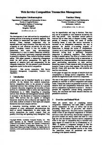
The inference algorithms are defined for a generic graph metamodel. The metamodel is a simplification of UML activity diagrams, and uses mostly the same notation. The new global and local performance constraints are represented as stereotyped annotations. A simplified UML class diagram for the ECore [7] graph metamodel is shown in figure 1. Graphs contain a set of FlowNodes and FlowEdges and have a manual global PerformanceAnnotation, which indicates all paths in the graph should finish in less than secsTimeLimit seconds while handling concurrentRequests requests concurrently. There are several kinds of FlowNodes:

Activities encapsulate some behavior, described textually in the attribute name. Activities can have manual or automatic performance annotations. Initial nodes are the starting execution points of the graphs. One per graph. Final nodes end the current execution branch. There can be more than one. Decision nodes select one execution branch among several, depending on whether the condition for their outgoing edge holds or not. Only the outgoing FlowEdges from a DecisionNode may have a non-empty condition and a probability less than 1. Fork nodes split the current execution branch into several parallel branches. Join nodes integrate several branches back into one, whether they started off from a decision node or a fork node. This is a simplification from UML, which uses different elements to integrate each kind of branch: join nodes and merge nodes, respectively.

0 ..*

Flo wEd g e co n d it io n : ESt rin g p ro b a b ilit y : EDo u b le Ob je ct

0 ..* o u t g o in g

0 ..* in co m in g Pe rfo rm a n ce An n o t a t io n co n cu rre n t Re q u e s t s : EDo u b le Ob je ct s e cs Tim e Lim it : EDo u b le Ob je ct m a n u a l : EBo o le a n

0 ..1 t a rg e t 0 ..1

Gra p h

0 ..*

Flo w No d e

0 ..1 s o u rce

0 ..1

Act ivit y n a m e : ESt rin g

In it ia lNo d e

Fin a lNo d e

Jo in No d e

Fo rkNo d e

De cis io n No d e

Fig. 1. Graph metamodel used in both algorithms

A sample model using this metamodel is shown in figure 2, which describes a process for handling an order. Execution starts from the initial node, and proceeds as follows: 1. The order is evaluated and is either accepted or rejected. 2. If rejected, close the order: we are done. 3. Otherwise, fork into 2 execution branches: (a) Create the shipping order and send it to the shipping partner. (b) Create the invoice, send it to the customer and receive its payment. 4. Once these 2 branches complete their execution, close the order. There are two manual performance annotations: a global one (using the stereotype) and a local one (using ). The whole process must be able to serve 5 concurrent requests in less than 1 second, and evaluating an order should be done in 0.4 seconds at most with 5 concurrent requests.

< < gpc> >

< < pc> >

concurrent Request s = 5

concurrent Request s = 4

t im eLim it = 1

t im eLim it = 0.4

m anual = t rue

m anual = false [ r e je ct e d] ( p = 0 .2 )

Evaluat e Order

Close Order

[ e lse ] ( p = 0 .8 ) Creat e Shipping Order

< < pc> >

< < pc> > concurrent Request s = 5

concurrent Request s = 5 t im eLim it = 0.4

Creat e Invoice

m anual = t rue

< < pc> >

Perform Paym ent

t im eLim it = 0.2 m anual = false

< < pc> >

concurrent Request s = 4

concurrent Request s = 4

t im eLim it = 0.2

t im eLim it = 0.2

m anual = false

m anual = false

Fig. 2. Sample graph model

3

Inference of concurrent requests

The first algorithm infers the number of concurrent requests that must be handled at each activity in the graph before its time limit in order to meet the performance requirements of the whole graph. It performs a pre-order breadthfirst traversal of every node and edge in the graph, starting from the initial node and caching intermediate results. The algorithm annotates each activity with its expected number of concurrent requests C(x). The definition of C(x) depends on the element type: – InitialNode: C(x) is the value of the attribute concurrentRequests of the global performance annotation of the graph. – FlowEdge: C(x) = P (x)C(s), where x is the edge, s is the source node of x, P (x) is the value of the attribute probability of x and C(s) is the computed number of concurrent requests for s. Most edges have P (x) = 1, except those which start from a decision node. – JoinNode: the least common ancestor LCA(P ) of all the parent nodes P is computed. This least common ancestor is the point from which the conditional P or parallel branches started off. If LCA(P ) is a decision node, C(x) = p∈P C(p), as requests can only visit one of the branches. Otherwise, it is a fork node, and C(x) = maxp∈P C(p), as requests can visit all the branches at the same time. To compute the LCA of several nodes, the naive method described by Bender et al. [8] works best for the sparse graphs which usually result from modeling service compositions. For a graph with n vertexes and e edges, its

preprocessing step requires O(n + e) operations and each query performed may require up to O(n2 ) operations. This only needs to be done once for each join node. – Otherwise, C(x) = C(i), where i is its only incoming edge. If the node is an activity with a manual performance annotation, the inferred value should match its value. Otherwise, the user will need to confirm if the annotation should be updated. Using these formulas, computing C(Create Invoice) for the example shown in figure 2 would require walking back to the initial node, finding an edge with a probability of p = 0.8, no merge nodes and a global performance annotation for G = 5 concurrent requests. Therefore, C(Create Invoice) = pG = 4.

4

Inference of time limits

The algorithm required to infer the time limits for each activity in the graph is more complicated than the previous one. It adds time limits to the activities in each path from the initial node to any of the final nodes, ensuring the inferred time limits meet several assumptions. This section starts with the requirements imposed on the results of the algorithm and lists the required definitions. The rest of the section describes the algorithm and shows an example of its application. 4.1

Design requirements

The inferred time limits must meet the following requirements: 1. The sum of the time limits of the activities in each path from the initial node to any of the final nodes must be less than or equal to the global time limit. 2. Available time should be split equally over the activities without any manual performance annotations. We cannot blindly assume that one activity will need to be more efficient than another. Ideally, we would like to split evenly the load over all activities. 3. Time limits should not be lower than strictly required: better performing systems tend to be more expensive to build and maintain. 4.2

Definitions

To describe the algorithm, several definitions are needed. These definitions consider paths as sets of activities, rather than sequences of nodes. – M (a) is true if the activity a has a manual time limit. – A(a) is true if the activity a has an automatic time limit. – U (p) = {a|a ∈ p ∧ ¬(A(a) ∨ M (a))} is the set of all activities in the path p which do not have time limits. These are said to be unrestricted.

– F (p) = {a|a ∈ p ∧ ¬M (a)} is the set of all activities in the path p which do not have manual time limits. These are said to be free. – TL (G) is the manual time limit for every path in the graph G. – TL (a) is the P current time limit for the activity a. – TL (p) = a∈P ∧(M (a)∨A(a)) TL (a) is the sum of the time limits in the path p. P – TM (p) = a∈(p−F (p)) TL (a) is defined as the sum of the manual time limits in the path p. – SA (p, G) = TL (G) − TM (p) is the slack which can be split among the free activities in path p of the graph G. – TE (p, G) = SA (p, G)/(1 + |F (p)|) is an estimate of the automatic time limit each free activity in path p would obtain using only the information in that path. More restrictive paths will have lower values of TE (p, G). 4.3

Description of the algorithm

The algorithm follows these steps: 1. All automatic time limits are removed. 2. The set P of all paths from the initial node to each final node is calculated. 3. For each path p ∈ P in ascending order of TE (p, G), so the more restrictive paths are visited first: (a) If SA (p, G) = 0, the condition |F (p)| > 0 is evaluated. If it is true, there is at least one free activity in p for which no time limit can be set. The user is notified of the situation and execution is aborted. Otherwise, processing will continue with the next path. (b) If SA (p, G) < 0, then TM (p) > TL (G) holds, by definition. This means that the sum of the manual time limits in p exceeds the global time limit. The user is notified of the situation and execution is aborted. (c) Otherwise, SA (p, G) > 0. If |F (p)| > 0 ∧ |U (p)| > 0, all activities in U (p) will be updated to the time limit (TL (G) − TL (p))/|U (p)|. 4.4

Example

To infer the automatic time limits of the running example shown in figure 2, we first need to list all existing paths: – p1 = {Evaluate Order, Close Order}. TE (p1 , G) = (1 − 0.4)/(1 + 1) = 0.3. – p2 = {Evaluate Order, Create Shipping Order, Close Order}. TE (p2 , G) = (1 − 0.4)/(1 + 2) = 0.2. – p3 = {Evaluate Order, Create Invoice, Receive Payment, Close Order}. TE (p3 , G) = (1 − 0.4)/(1 + 3) = 0.15. p3 has the lowest value for TE , so it is visited first. “Create Invoice”, “Perform Payment” and “Close Order” are in U (p3 ), so they are updated to l = (1 − 0.4)/3 = 0.2. p2 is visited next. Only “Create Shipping Order” is in U (p2 ), so it is updated to l = (1 − 0.6)/1 = 0.4. p1 is visited last. U (p1 ) = ∅, so nothing is updated, and we are done.

5

Integration in a SOA methodology

The algorithms described above work on a generic graph metamodel which needs to be adapted to the metamodels used in specific technologies and methodologies. In this section we show how the metamodel and the algorithms were adapted and integrated into a SOA methodology: SODM+Testing. Existing methodologies reduce the development cost of SOAs, but do not take testing aspects into account [9]. SODM+Testing is a new methodology that extends SODM [10] with testing tasks, techniques and models. 5.1

Metamodel adaptation

The original SODM service process and service composition metamodels were a close match to the generic graph metamodel described in section 2, as they were also based on UML activity graphs. Service process models described how a request for a service offered by the system should be handled, and service compositions provided details on how the tasks were split among the partners and what messages were exchanged between them. SODM+Testing refactors these models using the generic graph metamodel as their core. Each class in the SODM process and composition metamodels can now be upcasted to the matching class of the generic graph metamodel both inference algorithms are based on. For instance, ProcessFlowEdge (class of all flow edges in the SODM service process metamodel) has become a subclass of FlowEdge (class of all flow edges in the generic graph metamodel). The generic core differs slightly from that in figure 1. FlowEdges are split into ControlFlows and ObjectFlows, and performance annotations have also been split into several types according to their scope. In addition, the SODM+Testing service composition metamodel has been extended so activities can contain action sub-graphs with their own local and global performance annotations. 5.2

Tool implementation

SODM+T is a collection of Eclipse plug-ins that assists the SODM+Testing methodology with graphical editors for the SODM+Testing service process and composition models. It is available under the Eclipse Public License v1.0 [11]. To ensure the inference algorithms can be applied, models are validated automatically upon saving, showing the usual error and warning markers and Quick Fixes. Validation has been implemented using Epsilon Validation Language (EVL) scripts [12] and OCL constraints. The algorithms are implemented in the Epsilon Object Language (EOL) and can be launched from the contextual menu of the graphical editor. The EOL scripts include two supporting algorithms for detecting cycles in graphs and computing the least common ancestor of two nodes [8].

6

Evaluation

In this section we will evaluate each algorithm, pointing out their current limitations and how we plan to overcome them. Later on, we will evaluate their theoretical performance. Finally, we will discuss the current state of SODM+T. 6.1

Inference of concurrent requests

This algorithm performs a breadth-first traversal on the graph, and assumes the number of concurrent requests has already been computed for all parent nodes. For this reason, it is currently limited to acyclic graphs. We intend to extend the model to allow loops, limiting their maximum expected number of iterations. The algorithm requires edges to be manually annotated with probabilities. These could be simply initialized to assume each branch in each decision node has the same probability of being activated, in absence of other information. The algorithm assumes only the current workflow is being run, thereby providing a best-case scenario. More realistic estimations would be obtained if restrictions from all workflows in the system were aggregated. Assuming the naive LCA algorithm has been used, this algorithm completes its execution for a graph with n nodes after O(n3 ) operations, as its outer loop visits each node in the graph to perform O(n2 ) operations for JoinNodes and O(1) operations for the rest. This is a conservative upper bound, as the O(n2 ) time for the naive LCA algorithm is for dense graphs, which are uncommon in service compositions. 6.2

Inference of time limits

As there must be a finite number of paths in the graph, the current version requires the graph to be acyclic, just as the previous algorithm. The algorithm could reduce paths with loops to regular sequences, where the activities in the loop would be weighted to take into account the maximum expected number of iterations. The algorithm only estimates maximum deterministic time limits. Probability distributions are not computed, as it does not matter which path is actually executed: all paths should finish in the required time. In addition, the user cannot adjust the way in which the available slack is distributed to each task. For instance, the user might know that a certain task would usually take twice as much time as some other task. Weighting the activities as suggested above would also solve this problem. Finally, like the previous algorithm, the time limit inference algorithm is currently limited to the best-case scenario where only the current workflow is being run. A formal proof of the correctness of the time limit inference algorithm is outside the scope of this paper. Nevertheless, we can show that the results produced by the algorithm meet the three design requirements listed in § 4.1. We assume

the model is valid (acyclic and weakly connected, among other restrictions) and that the algorithm completes its execution successfully: 1. The first requirement is met by sorting the paths from most to least restrictive. For the i-th path pi , only the nodes for which pi provides the strictest constraints (that is, U (pi )) are updated so TL (pi ) < TL (G). Since the activities from the previous (and stricter) paths were not changed, TL (pj ) < TL (G), j ≤ i. Once all paths have been processed, TL (p) < TL (G) holds for all p ∈ P . 2. The second requirement is met by simply distributing equally the available slack using a regular division. 3. The third requirement is met by visiting the most restrictive paths first, so activities obtain the strictest time limits as soon as possible, leaving more slack for those who can use it. The running time of the algorithm is highly dependent on the number of unique paths in the graph. With no loss of generality, we assume all forks and decision nodes are binary. If there are b decision and fork nodes in total among the n nodes, there will be 2b unique paths to be considered. Enumerating the existing paths requires a depth-first traversal of the graph, which may have to consider the O(n2 ) edges in the graph. Each path in the graph will have to be traversed a constant number of times to compute TE (p, G), SA (p, G), |F (p)| and other formulas which require O(n) operations. Therefore, the algorithm requires O(n2 + n2b ) time. We can see that the number of forks and decisions has a large impact on the running time of the algorithm. This could be alleviated by culling paths subsumed in other paths. We are also looking into alternative formulations which do not require all paths to be enumerated. 6.3

SODM+T

SODM+T has been successfully used to model the abstract logic required to handle a business process from a medium-sized company, generating performance annotations for graphs with over 60 actions nested in several activities. However, SODM+T could be improved: future versions will address some of the issues found during this first experience. WSDL descriptions and test cases (for tools such as soapUI [13] or JUnitPerf [14]) need to be generated from the models. Performance annotations should be more fine-grained, letting the user specify only one of the attributes so the other is automatically inferred. Finally, the tools could be adapted to other metamodels more amenable to code generation. Business Process Modeling Notation [3] models are a good candidate, as partial automated translations to executable forms already exist [15].

7

Related work

Several UML profiles for modeling the expected performance of a system have been approved by the Object Management Group: SPTP [16], QFTP [17] and

MARTE [18]. To study the feasibility of our approach, we have kept our constraints much simpler, but we intend to adapt them to either SPTP or QFTP in the future. Existing works on performance estimation in workflows focus on aggregating workflow QoS from task QoS, unlike our approach, which estimates task QoS from workflow QoS. Silver et al. [19] annotated each task in a workflow with probability distributions for their running times, and collected data from 100 simulation runs to estimate the probability distribution of the running time of the workflow and validate it using a Kolmogorov-Smirnov goodness-of-fit test. Simulating the workflow allows for flexibly modeling the stochastic behavior of each service, but it has a high computational overhead due to the number of simulation runs that are required. Our work operates directly on the graph, imposing less computational overhead, but only modeling deterministic maximum values. Other authors convert workflows to an existing formalism and solve it using an external tool. The most common formalisms are layered queuing networks [20], stochastic Petri networks [21] and process algebra specifications [22]. These formalisms are backed by in-depth research and the last two have solid mathematical foundations in Markov chain theory. However, they introduce an additional layer of complexity which might discourage some users from applying these techniques. Our work operates on the models as-is, with no need for conversions. This makes them easier to understand. Finally, some authors operate directly on the workflow models, as our approach does. The SWR algorithm proposed by Cardoso et al. [4] computes workflow QoS by iteratively reducing its graph model to a single task. SWR only works with deterministic values, like our algorithms, but its QoS model is more detailed than ours, describing the cost, reliability and minimum, average and maximum times for each service. We argue that though average and minimum times might be useful for obtaining detailed estimations, they provide little value for top-down development, which is only interested in establishing a set of constraints which can be used for conducting load testing and monitoring for each service. However, cost and reliability could be interesting in this context as well. It is interesting to note that Cardoso et al. combine several data sources to estimate the QoS of each task [4]: designer experience, previous times in the current instance, previous times in all instances of this workflow, and previous times in all workflows. The designer is responsible for specifying the relative importance of each data source. Results from our algorithms could be used as yet another data source. Our metamodels have been integrated into SODM+Testing, a SOA modeldriven methodology which extends the SODM methodology [10] with testing aspects. Many other SOA methodologies exist: for instance, Erl proposes a highlevel methodology focused on governance aspects in his book [1] and IBM has defined the comprehensive (but proprietary) SOMA methodology [23]. SODM was selected as it is model-driven and strikes a balance between scope and cost.

8

Conclusions and future work

Service compositions allow several WS to be integrated as a single WS which can be flexibly reconfigured as business needs change. However, setting initial performance requirements for the integrated services in a top-down methodology so the entire composition works as expected without incurring additional costs is difficult. At an early stage of development, there is not enough information to use more comprehensive techniques. This work has presented the first version of two algorithms which infer missing information about response times under certain loads from models inspired in UML activity graphs. Though a formal proof was outside the scope of this paper, we have found them to meet their design requirements: they infer local constraints which meet the global constraints, distribute the load equally over the composition and allow for as much slack as possible. These algorithms and their underlying metamodel have been successfully integrated into a model-driven SOA methodology, continuing the previous work shown in [9]. The tools [11] implement a graphical editor which allows the user to define performance requirements at several levels and offers automated validation and transformation. Nevertheless, the algorithms and tools could be improved. The underlying metamodel should allow for partially automatic annotations and use weights for distributing the available slack between the activities. In the future, the annotations could be adapted to the OMG SPTP [16], QFTP [17] or MARTE [18] UML profiles. The algorithms will be revised to handle cyclic graphs and aggregate constraints for a service from several models. The performance of the time limit inference algorithm depends on the number of unique graphs from the initial node to each final node in the tree. We are looking into ways to reduce the number of paths which need to be checked. Finally, it is planned to adapt the tools to service composition models more amenable to executable code generation, such as BPMN [3], and to generate test cases for existing testing tools such as soapUI [13] or JUnitPerf [14].

References 1. Erl, T.: SOA: Principles of Service Design. Prentice Hall, Indiana, EEUU (2008) 2. OASIS: Web Service Business Process Execution Language (WS-BPEL) 2.0. http: //docs.oasis-open.org/wsbpel/2.0/OS/wsbpel-v2.0-OS.html (April 2007) 3. Object Management Group: Business Process Modeling Notation (BPMN) 1.2. http://www.omg.org/spec/BPMN/1.2/ (January 2009) 4. Cardoso, J., Sheth, A., Miller, J., Arnold, J., Kochut, K.: Quality of service for workflows and web service processes. Web Semantics: Science, Services and Agents on the World Wide Web 1(3) (April 2004) 281–308 5. Hwang, S., Wang, H., Tang, J., Srivastava, J.: A probabilistic approach to modeling and estimating the QoS of web-services-based workflows. Information Sciences 177(23) (2007) 5484–5503

6. Yu, T., Zhang, Y., Lin, K.: Efficient algorithms for web services selection with end-to-end QoS constraints. ACM Transactions on the Web 1(1) (2007) 7. Eclipse Foundation: Eclipse Modeling Framework. http://eclipse.org/ modeling/emf/ (2010) 8. Bender, M.A., Pemmasani, G., Skiena, S., Sumazin, P.: Finding least common ancestors in directed acyclic graphs. Proceedings of the 12th Annual ACM-SIAM Symposium on Discrete Algorithms (SODA’01) (2001) 845–853 9. García-Domínguez, A., Medina-Bulo, I., Marcos-Bárcena, M.: Hacia la integración de técnicas de pruebas en metodologías dirigidas por modelos para SOA. In: Actas de las V Jornadas Científico-Técnicas en Servicios Web y SOA, Madrid, España (October 2009) 10. de Castro, M.V.: Aproximación MDA para el desarrollo orientado a servicios de sistemas de información web: del modelo de negocio al modelo de composición de servicios web. PhD thesis, Universidad Rey Juan Carlos (March 2007) 11. García-Domínguez, A.: Homepage of the SODM+T project. https://neptuno. uca.es/redmine/projects/sodmt (March 2010) 12. Kolovos, D., Paige, R., Rose, L., Polack, F.: The Epsilon Book. http://www. eclipse.org/gmt/epsilon (2010) 13. eviware.com: Homepage of soapUI. http://www.soapui.org/ (2009) 14. Clark, M.: JUnitPerf. http://clarkware.com/software/JUnitPerf.html (October 2009) 15. Küster, T., Heßler, A.: Towards transformations from BPMN to heterogeneous systems. In Mecella, M., Yang, J., eds.: BPM2008 Workshop Proceedings, Milan, Italy (September 2008) 16. Object Management Group: UML Profile for Schedulability, Performance, and Time (SPTP) 1.1. http://www.omg.org/spec/SPTP/1.1/ (January 2002) 17. Object Management Group: UML Profile for Modeling Quality of Service and Fault Tolerance Characteristics and Mechanisms (QFTP) 1.1. http://www.omg. org/spec/QFTP/1.1/ (April 2008) 18. Object Management Group: UML Profile for Modeling and Analysis of RealTime Embedded systems (MARTE) 1.0. http://www.omg.org/spec/MARTE/1.0/ (November 2009) 19. Silver, G.A., Maduko, A., Rabia, J., Miller, J., Sheth, A.: Modeling and simulation of quality of service for composite web services. In: Proceedings of 7th World Multiconference on Systemics, Cybernetics and Informatics, International Institute of Informatics and Systems (November 2003) 20. Petriu, D.C., Shen, H.: Applying the UML Performance Profile: Graph Grammarbased Derivation of LQN Models from UML Specifications. In: Proceedings of the 12th International Conference on Computer Performance Evaluation: Modelling Techniques and Tools (TOOLS 2002). Volume 2324 of Lecture Notes in Computer Science. Springer Berlin, London, UK (2002) 159—177 21. López-Grao, J.P., Merseguer, J., Campos, J.: From UML activity diagrams to Stochastic Petri nets: application to software performance engineering. SIGSOFT Softw. Eng. Notes 29(1) (2004) 25–36 22. Tribastone, M., Gilmore, S.: Automatic extraction of PEPA performance models from UML activity diagrams annotated with the MARTE profile. In: Proceedings of the 7th International Workshop on Software and Performance, Princeton, NJ, USA, ACM (2008) 67–78 23. Ghosh, S., Arsanjani, A., Allam, A.: SOMA: a method for developing serviceoriented solutions. IBM Systems Journal 47(3) (2008) 377–396