progressive type-II censored samplesâ, The American Statistician, 49, 229â230. Chandrasekhar, B., Childs, A., Balakrishnan, N. (2004), âExact likelihood ...
Inference under progressively Type II right censored sampling for certain lifetime distributions Bing Xing Wang Zhejiang Gongshang University, P.R. China
Keming Yu Brunel University, UK
M.C. Jones The Open University, UK
Abstract In this paper, estimation of the parameters of a certain family of two-parameter lifetime distributions based on progressively Type II right censored samples (including ordinary Type II right censoring) is studied. This family, of reverse hazard distributions, includes the Weibull, Gompertz and Lomax distributions. A new type of parameter estimation, named inverse estimation, is introduced for both parameters. Exact confidence intervals for one of the parameters and generalized confidence intervals for the other are explored; inference for the first parameter can be accomplished by our methodology independently of the unknown value of the other parameter in this family of distributions. Derivation of the estimation method uses properties of order statistics. A simulation study in the particular context of the Weibull distribution illustrates the accuracy of these confidence intervals and compares inverse estimators favorably with maximum likelihood estimators. A numerical example is used to illustrate the proposed procedures. Key words: confidence interval, inverse estimator, order statistics, proportional reverse hazard distribution.
1
1
Introduction Lifetime distributions under censored sampling have been attracting great interest owing
to their wide application in sciences, engineering, social sciences, public health and medicine. It would be impossible to cite them all in a single paper. Take the simplest lifetime distribution — the one-parameter exponential distribution — as an example. Censored sampling associated with the exponential distribution has received much attention in the literature for many years (e.g. Saleh, 1967, Pettitt, 1977; Wright et al., 1978; Lam, 1994; Sundberg, 2001; Chandrasekhar et al., 2004; Balakrishnan et al., 2008). Censored data are of progressively Type II right type when they are censored by the removal of a prespecified number of survivors whenever an individual fails; this continues until a fixed number of failures has occurred, at which stage the remainder of the surviving individuals are also removed/censored. See, for example, Balakrishnan & Aggarwala (2000) and Balakrishnan (2007). This scheme includes ordinary Type II right censoring and complete data as special cases. Our methods not only apply to (progressively) Type II right censored data but also give new estimators in the complete data case. Let F (x; λ, α) be a lifetime distribution with parameters λ and α. Consider parameter estimation for the family with F (x; λ, α) = 1 − [1 − G(x; λ)]α
(1)
where G(·; λ) is a distribution function dependent only on λ. This family of distributions — without necessarily confining attention to a one-parameter G — is discussed in Marshall and Olkin (2007, Section 7.E. & ff.). They call (1) a ‘resilience parameter’ or ‘proportional reverse hazards’ family. When α is an integer, (1) is the distribution function of the minimum of a random sample of size α from the distribution G(·; λ). Examples of family (1) include the Weibull distribution, the Gompertz distribution and the Lomax distribution. For example, λ
when G(x; λ) = 1 − e−x in family (1), we have the two-parameter Weibull distribution. In the Gompertz and Lomax special cases, λ is the scale parameter and α the shape parameter; in the Weibull case, the roles of the parameters are reversed. We will call α the power parameter and λ the G-parameter. Maximum likelihood estimation (MLE) is a popular statistical method used for fitting these lifetime distributions, and confidence intervals for parameters of these distributions 2
under censored sampling are of particular interest in many applications. In this paper, in contrast to MLE, a new type of parameter estimation, named inverse estimation, is proposed for inference in the family of lifetime distributions under progressively Type II censored sampling, and their efficiency relative to MLE is investigated. Of particular interest is a neat method which is introduced to derive exact confidence intervals for the G-parameter λ, which is independent of the power parameter α. The paper is organized as follows. To make things clear, we first concentrate our discussion on the Weibull distribution, then generalize our work to the distribution family (1). Under progressively Type II right censoring, Section 2 gives exact confidence intervals for λ (independent of α), then gives generalized confidence intervals for α, as well as for other quantities (mean, quantiles and reliability function). A new type of parameter estimation, named inverse estimation, is introduced for both parameters. Section 3 extends the discussion to the family (1), including Gompertz and Lomax distributions. In Section 4.1, in the context of progressively Type II right censoring from the Weibull distribution we study by simulation the coverage probabilities of the proposed generalized confidence intervals for parameter α as well some important quantities of the distribution, and also compare the proposed estimators to MLE. In Section 4.2, a numerical example is given to illustrate the proposed procedures.
2
Progressive Type II right censoring from the Weibull distribution In this section, confidence intervals for the Weibull distribution are firstly derived in the
presence of progressively Type II right censored observations, then inverse estimators for both shape and scale parameters are introduced. Let the cumulative distribution function of the Weibull distribution Wei(λ, α) be given by λ
F (x; α, λ) = 1 − e−(αx) ,
x > 0,
where α > 0, λ > 0 are unknown parameters. Note that, in the Weibull case, α in (1) is reparameterized as αλ .
3
Suppose that n units are placed on a life test. Prior to the experiment, a number m (< n) P is fixed and the censoring scheme R = (R1 , R2 , . . . , Rm ) with Rj ≥ 0 and m j=1 Rj + m = n
is specified. At the first failure time X1:m:n , R1 units, chosen at random, are removed from the n − 1 surviving units. At the second failure time X2:m:n , R2 randomly chosen units from
the remaining n − 2 − R1 units are removed. The test continues until the mth failure time P Xm:m:n . At this time, all remaining units are removed; there are Rm = n − m − m−1 j=1 Rj
of these. The set of observed lifetimes X = (X1:m:n , X2:m:n , . . . , Xm:m:n ) is a progressively
Type II right censored sample. If R1 = R2 = . . . = Rm−1 = 0, then Rm = n − m which corresponds to the ordinary Type II right censoring scheme. If m = 0, there is no censoring. In order to derive our confidence intervals for the parameters λ and α as well as other quantities, the following well known properties of order statistics and Poisson processes are required: (I) If Vi:m:n = − log(1 − F (Xi:m:n ; α, λ)), i = 1, ..., m, then V1:m:n , . . . , Vm:m:n is a progressively Type II right censored sample from the standard exponential distribution with sample size n and censoring scheme R = (R1 , ..., Rm ). Note that, in the Weibull case, Vi:m:n = (αXi:m:n )λ . (II) If W1 = nV1:m:n , Wi = [n −
Pi−1
j=1 (Rj
+ 1)](Vi:m:n − Vi−1:m:n ), i = 2, . . . , m, then
W1 , . . . , Wm are independent standard exponential random variates. Pi (III) If Si = j=1 Wj , i = 1, . . . , m, and U(i) = Si /Sm , i = 1, . . . , m − 1, then
U(1) < . . . < U(m−1) are order statistics from the uniform (0, 1) distribution with sample P P size m − 1. Note that Si = ij=1(Rj + 1)Vj:m:n + [n − ij=1 (Rj + 1)]Vi:m:n , i = 1, . . . , m.
Fact (I) is obvious. Fact (II) can be found in Viveros & Balakrishnan (1994) and fact (III) in, for example, Stephens (1986).
2.1
Interval estimation of parameter λ
We now discuss interval estimation of the parameter λ. Consider the pivotal quantity W (λ) =
m−1 X
−2 log U(i) = 2
i=1 m−1 X
= 2
i=1
�
log
(
m−1 X
log (Sm /Si )
i=1
Pm
+ 1)Vj:m:n Pi Pi j=1 (Rj + 1)]Vi:m:n j=1 (Rj + 1)Vj:m:n + [n − 4
j=1 (Rj
)
= 2
m−1 X i=1
log
Pi
j=1 (Rj +
Pm
λ j=1 (Rj + 1)Xj:m:n P λ 1)Xj:m:n + [n − ij=1 (Rj
λ + 1)]Xi:m:n
(2)
From (2), it is of great importance to note that, for the Weibull distribution, W is a function of λ only and does not depend on α. It is clear that W (λ) can take any positive value. Moreover, it is also the case that W (λ) has the χ2 distribution with 2(m − 1) degrees of freedom. To see this, note that � Pm−1 P −2 log U = i=1 (−2 log Ui ) . And U1 , . . . , Um−1 form a random sample W (λ)= m−1 (i) i=1 from the uniform (0, 1) distribution.
It remains to show that W (λ) is a strictly monotonic function of λ. Write Q(j,i) = Vj:m:n /Vi:m:n = (Xj:m:n /Xi:m:n )λ . Note that Sm Sm − Si =1+ =1+ Si Si
Pm
j=i+1 (Rj Pi j=1 (Rj
P + 1)Q(j,i) − (n − ij=1(Rj + 1)) . P + 1)Q(j,i) + n − ij=1 (Rj + 1)
It is clear that W (λ) is a strictly increasing function of λ because Q(j,i) is strictly increasing (resp. decreasing) for j > (resp. 0, W −1 (t) is the solution in λ of the equation W (λ) = t.
2.2
Interval estimation of parameter α and other quantities
We now derive generalized confidence intervals for the parameter α and some important quantities of the Weibull distribution, such as its mean, quantiles and reliability function.
5
We utilise again the unique solution to W (λ) = t which we denote by g(W, X). Note also that V = 2Sm = 2αλ T (λ) has the χ2 distribution with 2m degrees of freedom, where T (λ) =
m X
λ (Rj + 1)Xj:m:n .
j=1
Therefore we have that α = (V /2T (λ))1/λ. According to the substitution method given by Weerahandi (1993, 2004), we substitute g(W, X) for λ in the expression for α and obtain the following generalized pivotal quantity for the parameter α: !1/g(W,x) V Y1 = , P g(W,x) 2 m j=1 (Rj + 1)xj:m:n
(3)
where x = (x1:m:n , ..., xm:m:n ) is the observed value of X = (X1:m:n , ..., Xm:m:n ). Notice that Y1 reduces to α when X = x, and the distribution of Y1 is free of any unknown parameters. If Y1,β denotes the upper β percentile of Y1 , then Y1,1−β and Y1,β are the 1 − β generalized lower and upper confidence limits for α, respectively. The values Y1,1−β and Y1,β can be obtained using Monte Carlo simulations. This can be done by using the following algorithm. For a given data set (n, m, x, R), generate W ∼ χ2 (2m − 2) and V ∼ χ2 (2m), independently. Using these values, we compute the values of Y1 in (3). This process of generating the value of Y1 is repeated m1 times for the fixed values of (n, m, x, R). Based on the generated values of Y1 , the values Y1,1−β and Y1,β can be obtained. Now note that the mean, pth quantile (0 < p < 1) and reliability function of the Weibull distribution are given by µ = Γ(1 + 1/λ)/α, xp = [− log(1 − p)]1/λ /α and R(x0 ) = exp[−(αx0 )λ ] respectively. Along the same lines as the derivation of Y1 for parameter α, we obtain the following generalized pivotal quantities Y2 , Y3 and Y4 for µ, xp and R(x0 ) respectively: Y2 =
Y3 =
2
Pm
g(W,x)
j=1 (Rj + 1)xj:m:n V
− log(1 − p) · 2
m X
1 ! g(W,x)
(Rj +
j=1
� Γ 1+
g(W,x) 1)xj:m:n /V
1 g(W, x)
1 ! g(W,x)
!
V g(W,x) . · x0 Y4 = exp − Pm g(W,x) 2 j=1 (Rj + 1)xj:m:n 6
,
�
,
(4)
(5)
(6)
Let Y2,β , Y3,β , Y4,β denote the upper β percentiles of Y2 , Y3, Y4 respectively. Then Y2,β , Y3,β , Y4,β are the 1 − β lower confidence limits for µ, xp and R(x0 ), respectively. Just as in the case of Y1 , the percentiles of Y2 , Y3, Y4 can be obtained by Monte Carlo simulations. Although the distributions of Y1 , Y2, Y3 , Y4 do not depend on any unknown parameters, the coverage probabilities of their generalized confidence intervals may depend on nuisance parameters. We study the performance of coverage probabilities of these confidence intervals by simulation. Such simulation results are reported in Section 4.1.
2.3
Inverse estimation of parameters λ and α
Since W (λ) has the χ2 distribution with 2(m − 1) degrees of freedom, W (λ)/ {2(m − 2)} converges with probability one to 1. Therefore, we can obtain a correspondˆ of λ from the following equation: ing point estimator λ ˆ = 2(m − 2). W (λ)
(7)
By the results in Section 2.1, equation (7) has a unique solution. Also, again using the fact that 2Sm has the χ2 distribution with 2m degrees of freedom, we obtain estimator α ˆ of α from the following equation: !1/λˆ m−1 α ˆ= . ˆ T (λ)
(8)
The estimators given by (7) and (8) are named as inverse estimators (IE) of parameters (Wang, 1992) and we continue to use this terminology here. We shall study the finite sample properties of the proposed estimators in Section 4. They turn out to be very good and consistently supeerior to MLEs. ˆ ˆ and [log(ˆ ˆ are Remark: It is easy to prove that λ/λ, [log(α) ˆ − log(α)]/λ xp ) − log(xp )]/λ pivotal quantities for the parameters λ, α and xp respectively. Hence, confidence intervals for these parameters can alternatively be obtained based on these pivotal quantities. The percentiles of these pivotal quantities can also be obtained by Monte Carlo simulations. This approach is much more computationally intensive than our exact confidence interval for λ while there is no alternative pivotal quantity, and hence no alternative condifence interval, for µ. This is very similar to the approach taken in the maximum likelihood case in Balakrishnan et al. (2004), except that the latter work uses the inferior MLEs instead of IEs. 7
3
Parameter estimation for the general family of lifetime distributions As we saw in Section 2 in the case of the Weibull distribution, we basically start with
′ m uniform order statistics in the shape of U(i) = F (Xi:m:n ; α, λ), i = 1, ..., m, and then go
through a series of transformations to get back to uniform order statistics again, this time m − 1 of them, U(i) , i = 1, ..., m − 1. The beauty of this, however, turned out to be that ′ while a summary statistic based directly on the U(i) depends on both α and λ, the final
summary statistic based on the U(i) ’s depends only on λ. This neat way can be generalized to progressively Type II censored sample from family (1), as follows. If X = (X1:m:n , X2:m:n , ..., Xm:m:n ) is a progressively Type II censored sample from distribution (1) with sample size n and censoring scheme R = (R1 , R2 , ..., Rm ), they can be accommodated by defining V(i) = − log(1 − F (Xi:m:n ; α, λ)) = −α log(1 − G(Xi:m:n ; λ)),
i = 1, ..., m,
in Step (I) of the development in Section 2. Everything else will follow through much as in Section 2 for the Weibull distribution. For example, W (λ) = 2
m−1 X
log (Tm /Ti ) ,
i=1
where Ti =
i X
(Rj +1) log[1−G(Xj:m:n ; λ)]+[n−
j=1
i X
(Rj +1)] log[1−G(Xi:m:n ; λ)], i = 1, ..., m. (9)
j=1
The key remains that α does not appear in this formula. Otherwise, we need to show on a case-by-case basis that W (λ) is a strictly monotone function of λ. This in turn will follow from showing that Q(i,j) = Vi::m:n /Vj:m:n is a strictly monotone function of λ for i < j. If the Q(i,j) , i < j, are monotone decreasing, then Theorem 1 applies as it is; if the Q(i,j) , i < j, are monotone increasing, then Theorem 1 applies with confidence limits reversed. For inference on α and other quantities depending on α as well as λ, note that in general V = 2αT (λ) where T (λ) =
m X (Rj + 1){− log(1 − G(Xi:m:n ; λ))}. j=1
8
Notice that what was αλ in V in the Weibull case has reverted to α in general. This means that the pivotal quantities in the work on generalized confidence intervals are changed a little (the power of 1/λ or 1/g(W, x) is not taken). For example, the generalized pivotal quantity for inference on the parameter α itself is Y1 =
2
V . j=1 (Rj + 1){− log(1 − G(xi:m:n ; g(W, x)))}
Pm
(10)
Equation (7) continues to give the point estimate of λ while ˆ α ˆ = (m − 1)/T (λ)
(11)
with the above definition of T (λ). Example 3.1: Progressive Type II right censoring from the Gompertz distribution The Gompertz distribution is of family (1) with G(x; λ) = 1 − exp(1 − eλx ). Thus, Vi;m;n = α(eλXi:m:n − 1) and Q(i,j) =
eλXi;m;n − 1 , eλXj:m;n − 1
i = 1, ..., m.
Lemma 1 below shows that Q(i,j) is strictly decreasing in λ for i < j and hence that Theorem 1 applies. Lemma 1 Let f (λ) = (eaλ − 1)/(ebλ − 1), where b > a > 0 are constants. Then f (λ) is strictly decreasing on (0, ∞). Proof.
f (λ) = g(λ)(eaλ − 1)/(ebλ − 1) where g(λ) =
a b − . −aλ 1−e 1 − e−bλ
From consideration of its derivative with respect to a, it is straightforward to see that a/(1 − e−aλ ) is strictly decreasing in a for λ > 0 so that g(λ) < 0 and the result follows. � Example 3.2: Progressive Type II right censoring from the Lomax distribution The Lomax (or Pareto II) distribution is of family (1) with G(x; λ) = λx/(1 + λx). This time, Q(i,j) = log(1 + λX(i) )/ log(1 + λX(j) ) proves to be strictly increasing in λ (proof not 9
given to save space) and hence W (λ) is a strictly decreasing function of λ. The resulting confidence interval for λ is therefore of the reversed form � −1 2 � W {χβ/2 (2(n − r − 1))}, W −1{χ21−β/2 (2(n − r − 1))} .
Remark: A parallel development is available for the less practically important situation of Type II left censored data from distributions of the form F (x; λ, α) = [G(x; λ)]α (such as the generalized exponential distribution, Gupta & Kundu, 1999).
4
Numerical analysis
4.1
Simulation study
In order to assess the finite sample properties of the proposed procedures, a simulation study was conducted to study the coverage probabilities of the proposed generalized confidence intervals and to compare the performance of the proposed point estimators with maximum likelihood estimators for the Weibull distribution under a variety of progressively Type II right censored sampling schemes. (There is no need to perform a simulation study of coverage of our intervals for λ because they are exact.) Since α is the scale parameter and estimators are appropriately scale equi- and in-variant, we take α = 1 in our simulation study and consider different values of λ. For different choices of sample sizes and censoring schemes, we generated progressively Type-II censored samples from the Weibull distribution using the algorithm presented in Balakrishnan and Sandhu (1995). We report the coverage probabilities of the generalized confidence intervals at 0.9 and 0.95 confidence levels for each of α, x0.1 , µ and R(1.2) in Tables 1–3. These were computed over 1,000 replications for each different case using m1 = 10, 000. Clearly, from so many different combinations of censoring schemes and sample sizes, the simulated probabilities for 0.9 and those for 0.95 are quite close to 0.9 and 0.95 respectively. We also report the average relative biases and average relative mean square errors (MSEs) in point estimation of α and λ over 10,000 replications for the same set of cases. The results are presented in Tables 4–6. Again it is quite clear from all three tables that, for a fixed sample size, as right censored number r increase the average relative biases and average relative MSEs increase as expected. It is also clear that the average biases and the average 10
Table 1: The coverage probabilities of the generalized confidence intervals when λ = 0.6 α
x0.1
µ
R(1.2)
(n, m)
(r1 , ..., rm )
0.90
0.90
0.95
(10,5)
(0,...,0,5)
0.887 0.945 0.917 0.961 0.879 0.928 0.888
0.947
(10,5)
(5,0,...,0)
0.898 0.946 0.901 0.947 0.886 0.933 0.899
0.945
(10,5)
(1,1,...,1)
0.898 0.939 0.899 0.947 0.888 0.937 0.901
0.940
(10,8)
(0,...,0,2)
0.887 0.944 0.902 0.946 0.888 0.946 0.890
0.947
(10,8)
(2,0,...,0)
0.904 0.957 0.897 0.948 0.896 0.943 0.907
0.956
(20,10)
(0,...,0,10)
0.894 0.947 0.882 0.944 0.895 0.951 0.893
0.944
(20,10)
(10,0,...,0)
0.899 0.950 0.886 0.954 0.910 0.951 0.900
0.951
(20,10)
(1,1,...,1)
0.905 0.951 0.896 0.938 0.889 0.952 0.900
0.950
(20,15)
(0,...,0,5)
0.909 0.959 0.904 0.944 0.902 0.961 0.909
0.959
(20,15)
(5,0,...,0)
0.905 0.958 0.903 0.944 0.914 0.961 0.905
0.958
(30,10)
(0,...,0,20)
0.914 0.958 0.892 0.944 0.904 0.954 0.913
0.958
(30,10)
(20,0,...,0)
0.896 0.950 0.891 0.953 0.911 0.953 0.898
0.952
(30,10)
(2,2,...,2)
0.913 0.954 0.893 0.947 0.906 0.954 0.910
0.954
(30,15)
(0,...,0,15)
0.911 0.955 0.899 0.948 0.897 0.942 0.908
0.958
(30,15)
(15,0,...,0)
0.906 0.957 0.905 0.945 0.911 0.961 0.907
0.957
(30,15)
(1,1,...,1)
0.912 0.958 0.909 0.944 0.902 0.956 0.919
0.962
(30,20)
(0,...,0,10)
0.905 0.955 0.907 0.955 0.890 0.949 0.907
0.949
(30,20)
(10,0,...,0)
0.898 0.950 0.891 0.948 0.900 0.949 0.897
0.951
(30,20) (5,0,...,0,5)
0.892 0.953 0.896 0.946 0.904 0.954 0.901
0.950
(50,12)
(0,...,0,38)
0.890 0.952 0.899 0.947 0.892 0.950 0.891
0.950
(50,12)
(38,0,...,0)
0.886 0.945 0.897 0.952 0.883 0.944 0.878
0.948
(50,20)
(0,...,0,30)
0.896 0.952 0.913 0.959 0.898 0.953 0.899
0.952
(50,20)
(30,0,...,0)
0.916 0.954 0.896 0.947 0.905 0.952 0.919
0.954
(50,25)
(0,...,0,25)
0.904 0.959 0.912 0.962 0.897 0.951 0.906
0.959
(50,25)
(25,0,...,0)
0.873 0.939 0.884 0.938 0.890 0.944 0.881
0.941
(50,25)
(1,1,...,1)
0.899 0.955 0.911 0.957 0.910 0.952 0.897
0.951
0.95
0.90
0.95
11
0.90
0.95
Table 2: The coverage probabilities of the generalized confidence intervals when λ = 1 α
x0.1
µ
R(1.2)
(n, m)
(r1 , ..., rm )
0.90
0.90
0.95
(10,5)
(0,...,0,5)
0.904 0.949 0.895 0.948 0.877 0.932 0.899
0.942
(10,5)
(5,0,...,0)
0.884 0.938 0.897 0.946 0.877 0.934 0.884
0.936
(10,5)
(1,1,...,1)
0.902 0.951 0.894 0.947 0.885 0.936 0.899
0.949
(10,8)
(0,...,0,2)
0.895 0.958 0.914 0.959 0.898 0.949 0.906
0.956
(10,8)
(2,0,...,0)
0.898 0.936 0.879 0.942 0.891 0.942 0.901
0.941
(20,10)
(0,...,0,10)
0.902 0.946 0.894 0.945 0.897 0.944 0.903
0.945
(20,10)
(10,0,...,0)
0.899 0.950 0.886 0.954 0.908 0.955 0.899
0.951
(20,10)
(1,1,...,1)
0.912 0.955 0.890 0.951 0.912 0.951 0.913
0.953
(20,15)
(0,...,0,5)
0.893 0.943 0.920 0.956 0.886 0.943 0.893
0.946
(20,15)
(5,0,...,0)
0.909 0.954 0.902 0.946 0.906 0.952 0.908
0.950
(30,10)
(0,...,0,20)
0.884 0.951 0.896 0.944 0.882 0.948 0.885
0.951
(30,10)
(20,0,...,0)
0.884 0.940 0.910 0.954 0.875 0.939 0.881
0.942
(30,10)
(2,2,...,2)
0.915 0.954 0.888 0.952 0.908 0.956 0.913
0.956
(30,15)
(0,...,0,15)
0.918 0.960 0.908 0.947 0.902 0.956 0.914
0.963
(30,15)
(15,0,...,0)
0.906 0.957 0.905 0.945 0.905 0.960 0.906
0.958
(30,15)
(1,1,...,1)
0.912 0.958 0.909 0.944 0.906 0.961 0.917
0.961
(30,20)
(0,...,0,10)
0.905 0.955 0.907 0.955 0.896 0.945 0.904
0.949
(30,20)
(10,0,...,0)
0.909 0.955 0.890 0.950 0.899 0.953 0.908
0.953
(30,20) (5,0,...,0,5)
0.901 0.951 0.907 0.953 0.897 0.947 0.905
0.955
(50,12)
(0,...,0,38)
0.904 0.945 0.901 0.948 0.894 0.947 0.900
0.946
(50,12)
(38,0,...,0)
0.903 0.954 0.901 0.949 0.899 0.956 0.902
0.956
(50,20)
(0,...,0,30)
0.903 0.949 0.896 0.949 0.896 0.948 0.904
0.949
(50,20)
(30,0,...,0)
0.908 0.955 0.920 0.959 0.899 0.946 0.904
0.943
(50,25)
(0,...,0,25)
0.904 0.939 0.900 0.960 0.895 0.944 0.901
0.940
(50,25)
(25,0,...,0)
0.907 0.956 0.913 0.960 0.908 0.955 0.900
0.955
(50,25)
(1,1,...,1)
0.899 0.955 0.911 0.957 0.897 0.956 0.902
0.949
0.95
0.90
12
0.95
0.90
0.95
Table 3: The coverage probabilities of the generalized confidence intervals when λ = 2 α
x0.1
µ
R(1.2)
(n, m)
(r1 , ..., rm )
0.90
0.90
0.95
(10,5)
(0,...,0,5)
0.904 0.949 0.895 0.948 0.886 0.935 0.900
0.942
(10,5)
(5,0,...,0)
0.884 0.938 0.897 0.946 0.877 0.931 0.880
0.941
(10,5)
(1,1,...,1)
0.902 0.952 0.895 0.947 0.887 0.938 0.899
0.942
(10,8)
(0,...,0,2)
0.887 0.943 0.891 0.947 0.890 0.941 0.902
0.941
(10,8)
(2,0,...,0)
0.904 0.952 0.901 0.945 0.891 0.938 0.902
0.945
(20,10)
(0,...,0,10)
0.905 0.960 0.901 0.949 0.897 0.955 0.915
0.961
(20,10)
(10,0,...,0)
0.891 0.951 0.897 0.952 0.877 0.935 0.908
0.945
(20,10)
(1,1,...,1)
0.908 0.958 0.905 0.948 0.905 0.957 0.910
0.961
(20,15)
(0,...,0,5)
0.903 0.946 0.896 0.951 0.888 0.939 0.901
0.948
(20,15)
(5,0,...,0)
0.843 0.947 0.893 0.952 0.895 0.942 0.899
0.952
(30,10)
(0,...,0,20)
0.914 0.958 0.892 0.944 0.910 0.955 0.903
0.955
(30,10)
(20,0,...,0)
0.899 0.961 0.909 0.960 0.901 0.961 0.897
0.954
(30,10)
(2,2,...,2)
0.905 0.963 0.884 0.946 0.899 0.959 0.903
0.962
(30,15)
(0,...,0,15)
0.903 0.950 0.903 0.951 0.894 0.946 0.897
0.946
(30,15)
(15,0,...,0)
0.887 0.948 0.900 0.948 0.895 0.947 0.891
0.943
(30,15)
(1,1,...,1)
0.892 0.947 0.905 0.939 0.887 0.946 0.896
0.949
(30,20)
(0,...,0,10)
0.902 0.951 0.895 0.958 0.876 0.943 0.881
0.943
(30,20)
(10,0,...,0)
0.888 0.948 0.889 0.951 0.879 0.934 0.897
0.953
(30,20) (5,0,...,0,5)
0.903 0.951 0.903 0.895 0.889 0.944 0.898
0.948
(50,12)
(0,...,0,38)
0.907 0.957 0.887 0.954 0.906 0.956 0.913
0.960
(50,12)
(38,0,...,0)
0.891 0.947 0.905 0.956 0.886 0.957 0.912
0.958
(50,20)
(0,...,0,30)
0.904 0.948 0.894 0.945 0.903 0.949 0.897
0.942
(50,20)
(30,...,0,0)
0.910 0.955 0.907 0.953 0.910 0.954 0.901
0.955
(50,25)
(0,...,0,25)
0.902 0.948 0.911 0.958 0.903 0.949 0.904
0.952
(50,25)
(25,0,...,0)
0.907 0.956 0.913 0.960 0.904 0.959 0.903
0.952
(50,25)
(1,1,...,1)
0.899 0.955 0.911 0.957 0.897 0.956 0.902
0.949
0.95
0.90
13
0.95
0.90
0.95
Table 4: The relative biases and relative MSEs of the estimators of Wei(0.6, 1) Bias
MSE
α
λ
α
λ
(n, m)
(r1 , ..., rm )
(10,5)
(0,...,0,5)
0.0278 1.1415 -0.0168 0.5555 3.2281 10.3066 0.3882 1.2780
(10,5)
(5,0,...,0)
0.1987 0.7841 -0.0425 0.2810 2.4319
5.5694
0.1702 0.3780
(10,5)
(1,1,...,1)
0.0648 0.9706 -0.0263 0.4322 2.7846
7.9178
0.2852 0.8031
(10,8)
(0,...,0,2)
0.0850 0.3844 -0.0138 0.2477 0.7509
1.3362
0.1348 0.2770
(10,8)
(2,0,...,0)
0.1707 0.3539 -0.0204 0.1930 0.9019
1.4128
0.1012 0.1871
(20,10)
(0,...,0,10)
0.0089 0.4299 -0.0072 0.2123 0.6086
1.2050
0.1253 0.2310
(20,10)
(10,0,...,0)
0.1275 0.2849 -0.0205 0.1147 0.5425
0.8495
0.0633 0.0937
(20,10)
(1,1,...,1)
0.0387 0.3646 -0.0128 0.1645 0.5171
0.9441
0.0911 0.1507
(20,15)
(0,...,0,5)
0.0389 0.1853 -0.0038 0.1215 0.2748
0.3850
0.0626 0.0938
(20,15)
(5,0,...,0)
0.0914 0.1666 -0.0085 0.0916 0.3177
0.3978
0.0457 0.0633
(30,10)
(0,...,0,20)
0.0368 0.6516 -0.0059 0.2241 1.0260
2.3507
0.1337 0.2525
(30,10)
(20,0,...,0)
0.1228 0.3156 -0.0232 0.0939 0.5363
0.8239
0.0531 0.0741
(30,10)
(2,2,...,2)
0.0350 0.4861 -0.0128 0.1645 0.7158
1.4503
0.0911 0.1507
(30,15)
(0,...,0,15)
0.0118 0.2699 -0.0023 0.1339 0.3485
0.5674
0.0702 0.1085
(30,15)
(15,0,...,0)
0.0877 0.1798 -0.0110 0.0766 0.3092
0.3941
0.0391 0.0519
(30,15)
(1,1,...,1)
0.0314 0.2265 -0.0061 0.1044 0.2978
0.4510
0.0519 0.0740
(30,20)
(0,...,0,10)
0.0158 0.1434 -0.0029 0.0911 0.1845
0.2480
0.0468 0.0641
(30,20)
(10,0,...,0)
0.0659 0.1204 -0.0073 0.0641 0.2075
0.2442
0.0319 0.0402
(30,20) (5,0,...,0,5) 0.0337 0.1281 -0.0049 0.0791 0.1816
0.2310
0.0404 0.0535
(50,12)
(0,...,0,38)
0.0709 0.7059 -0.0054 0.1835 1.0784
2.5448
0.1014 0.1773
(50,12)
(38,0,...,0)
0.1008 0.2556 -0.0201 0.0674 0.4162
0.6020
0.0382 0.0494
(50,20)
(0,...,0,30)
0.0057 0.2370 -0.0018 0.0997 0.2876
0.4442
0.0522 0.0732
(50,20)
(30,0,...,0)
0.0632 0.1285 -0.0092 0.0524 0.2021
0.2446
0.0273 0.0331
(50,25)
(0,...,0,25)
0.0006 0.1446 -0.0018 0.0754 0.1688
0.2274
0.0392 0.0510
(50,25)
(25,0,...,0)
0.0501 0.0947 -0.0068 0.0449 0.1502
0.1765
0.0233 0.0274
(50,25)
(1,1,...,1)
0.0137 0.1208 -0.0041 0.0585 0.1415
0.1820
0.0289 0.0352
IE
MLE
IE
14
MLE
IE
MLE
IE
MLE
Table 5: The relative biases and relative MSEs of the estimators of Wei(1, 1) Bias
MSE
α
λ
α
λ
(n, m)
(r1 , ..., rm )
(10,5)
(0,...,0,5)
-0.1271 0.4180 -0.0168 0.5555 0.4648 0.9675 0.3882 1.2780
(10,5)
(5,0,...,0)
0.0129
(10,5)
(1,1,...,1)
-0.0829 0.3605 -0.0263 0.4322 0.3988 0.7958 0.2852 0.8031
(10,8)
(0,...,0,2)
-0.0028 0.1549 -0.0138 0.2477 0.1702 0.2495 0.1348 0.2770
(10,8)
(2,0,...,0)
0.0428
(20,10)
(0,...,0,10)
-0.0478 0.1836 -0.0072 0.2123 0.1636 0.2428 0.1253 0.2310
(20,10)
(10,0,...,0)
0.0335
(20,10)
(1,1,...,1)
-0.0209 0.1572 -0.0128 0.1645 0.1369 0.1997 0.0911 0.1507
(20,15)
(0,...,0,5)
-0.0022 0.0802 -0.0038 0.1215 0.0789 0.0977 0.0626 0.0938
(20,15)
(5,0,...,0)
0.0270
(30,10)
(0,...,0,20)
-0.0592 0.2682 -0.0059 0.2241 0.2517 0.4098 0.1337 0.2525
(30,10)
(20,0,...,0)
0.0310
(30,10)
(2,2,...,2)
-0.0371 0.2074 -0.0128 0.1645 0.1806 0.2776 0.0911 0.1507
(30,15)
(0,...,0,15)
-0.0262 0.1197 -0.0023 0.1339 0.1019 0.1346 0.0702 0.1085
(30,15)
(15,0,...,0)
0.0253
(30,15)
(1,1,...,1)
-0.0090 0.1010 -0.0061 0.1044 0.0855 0.1107 0.0519 0.0740
(30,20)
(0,...,0,10)
-0.0093 0.0641 -0.0029 0.0911 0.0574 0.0686 0.0468 0.0641
(30,20)
(10,0,...,0)
0.0196
0.0507 -0.0073 0.0641 0.0612 0.0678 0.0319 0.0402
(30,20) (5,0,...,0,5)
0.0021
0.0560 -0.0049 0.0791 0.0556 0.0648 0.0404 0.0535
(50,12)
(0,...,0,38)
-0.0456 0.2874 -0.0054 0.1835 0.2717 0.4530 0.1014 0.1773
(50,12)
(38,0,...,0)
0.0259
(50,20)
(0,...,0,30)
-0.0260 0.1063 -0.0018 0.0997 0.0894 0.1133 0.0522 0.0732
(50,20)
(30,0,...,0)
0.0185
(50,25)
(0,...,0,25)
-0.0176 0.0661 -0.0018 0.0754 0.0546 0.0642 0.0392 0.0510
(50,25)
(25,0,...,0)
0.0149
(50,25)
(1,1,...,1)
-0.0067 0.0554 -0.0041 0.0585 0.0453 0.0527 0.0289 0.0352
IE
MLE
IE
MLE
IE
MLE
IE
MLE
0.2901 -0.0425 0.2811 0.3549 0.6474 0.1702 0.3779
0.1435 -0.0204 0.1933 0.1913 0.2552 0.1012 0.1870
0.1246 -0.0205 0.1149 0.1353 0.1773 0.0633 0.0936
0.0699 -0.0085 0.0916 0.0868 0.0996 0.0457 0.0632
0.1334 -0.0232 0.0939 0.1341 0.1805 0.0531 0.0741
0.0765 -0.0110 0.0766 0.0848 0.0998 0.0391 0.0519
0.1097 -0.0201 0.0674 0.1083 0.1394 0.0382 0.0494
0.0557 -0.0092 0.0524 0.0598 0.0676 0.0273 0.0331
0.0413 -0.0068 0.0450 0.0463 0.0506 0.0233 0.0274
15
Table 6: The relative biases and relative MSEs of the estimators of Wei(2.0, 1) Bias
MSE
α
λ
α
λ
(n, m)
(r1 , ..., rm )
(10,5)
(0,...,0,5)
-0.1163 0.1477 -0.0168 0.5555 0.1055 0.1226 0.3882 1.2780
(10,5)
(5,0,...,0)
-0.0257 0.1000 -0.0425 0.2811 0.0642 0.0902 0.1702 0.3779
(10,5)
(1,1,...,1)
-0.0827 0.1280 -0.0263 0.4322 0.0824 0.1045 0.2852 0.8031
(10,8)
(0,...,0,2)
-0.0195 0.0554 -0.0138 0.2477 0.0361 0.0440 0.1348 0.2770
(10,8)
(2,0,...,0)
0.0024
(20,10)
(0,...,0,10)
-0.0435 0.0699 -0.0072 0.2123 0.0392 0.0438 0.1253 0.2310
(20,10)
(10,0,...,0)
0.0024
(20,10)
(1,1,...,1)
-0.0261 0.0601 -0.0128 0.1645 0.0313 0.0369 0.0911 0.1507
(20,15)
(0,...,0,5)
-0.0102 0.0300 -0.0038 0.1215 0.0181 0.0201 0.0626 0.0938
(20,15)
(5,0,...,0)
0.0039
(30,10)
(0,...,0,20)
-0.0603 0.0997 -0.0059 0.2241 0.0615 0.0687 0.1337 0.2525
(30,10)
(20,0,...,0)
0.0012
(30,10)
(2,2,...,2)
-0.0395 0.0794 -0.0128 0.1645 0.0419 0.0486 0.0911 0.1507
(30,15)
(0,...,0,15)
-0.0253 0.0465 -0.0023 0.1339 0.0244 0.0267 0.0702 0.1085
(30,15)
(15,0,...,0)
0.0033
(30,15)
(1,1,...,1)
-0.0144 0.0394 -0.0061 0.1044 0.0198 0.0223 0.0519 0.0740
(30,20)
(0,...,0,10)
-0.0115 0.0246 -0.0029 0.0911 0.0137 0.0148 0.0468 0.0641
(30,20)
(10,0,...,0)
0.0028
IE
MLE
IE
MLE
IE
MLE
IE
MLE
0.0492 -0.0204 0.1933 0.0380 0.0452 0.1012 0.1870
0.0454 -0.0205 0.1149 0.0287 0.0338 0.0633 0.0936
0.0245 -0.0085 0.0916 0.0191 0.0208 0.0457 0.0632
0.0496 -0.0232 0.0939 0.0286 0.0342 0.0531 0.0741
0.0279 -0.0110 0.0766 0.0187 0.0207 0.0391 0.0519
0.0179 -0.0073 0.0641 0.0140 0.0148 0.0319 0.0402
(30,20) (5,0,...,0,5) -0.0055 0.0209 -0.0049 0.0791 0.0130 0.0141 0.0404 0.0535 (50,12)
(0,...,0,38)
-0.0564 0.1053 -0.0054 0.1835 0.0672 0.0769 0.1014 0.1773
(50,12)
(38,0,...,0)
0.0012
(50,20)
(0,...,0,30)
-0.0240 0.0414 -0.0018 0.0997 0.0220 0.0234 0.0522 0.0732
(50,20)
(30,0,...,0)
0.0024
(50,25)
(0,...,0,25)
-0.0155 0.0260 -0.0018 0.0754 0.0134 0.0140 0.0392 0.0510
(50,25)
(25,0,...,0)
0.0021
(50,25)
(1,1,...,1)
-0.0088 0.0219 -0.0041 0.0585 0.0109 0.0117 0.0289 0.0352
0.0412 -0.0201 0.0674 0.0235 0.0274 0.0382 0.0494
0.0205 -0.0092 0.0524 0.0137 0.0147 0.0273 0.0331
0.0149 -0.0068 0.0450 0.0108 0.0114 0.0233 0.0274
16
MSEs decrease as sample size increases. But the most striking information given by the simulation results is that the proposed inverse estimators outperform the maximum likelihood estimators from both bias and MSE viewpoints in all cases. The two differ less for larger n. For λ, the positive finite sample bias of the MLE is replaced by a smaller negative bias for the IE. For α, more (small) negative, as opposed to positive, biases are obtained as λ increases. According to these simulation results, we suggest using the proposed estimators, having particular merit for small and moderate sample sizes.
4.2
An illustrative example
Let us consider the data on times to breakdown of an insulating fluid from Table 1 of Viveros and Balakrishnan (1994) which is also reproduced in Balakrishnan et al. (2004) and Balakrishnan (2007). These data were artifically progressively censored by Viveros and Balakrishnan from a complete dataset given in Table 6.1 of Nelson (1982). Here, n = 19, m = 8 and R = (0, 0, 3, 0, 3, 0, 0, 5). Following each of these previous authors, we assume that the lifetimes follow the Weibull distribution. According to Section 3.2 of Viveros and Balakrishnan (1994), the MLEs of α ˆ M = 1/1.026 ≃ 0.97, respectively. Viveros and Balakrand λ are α ˆ M = e−2.222 ≃ 0.11 and λ ishnan also give a (conditional) 90% confidence interval for the parameter λ as (0.46, 1.38) and a (conditional) 95% confidence interval for the parameter α as (0.02, 0.20); Balakrishnan et al. (2004) obtain very similar confidence intervals by their unconditional approach based on the MLE. ˆ = 0.76, respectively. The inverse estimators of α and λ, on the other hand, are α ˆ = 0.08, λ Clearly, the inverse estimators for parameters (α, λ) are quite different from their MLEs. We have good reason to claim that the inverse estimators are preferable because the inverse estimators are very close to the IEs based on the complete sample which are α ˆ = 0.08 and ˆ = 0.73 (the MLEs based on the complete sample are α ˆ M = 0.77). λ ˆM = 0.04 and λ According to Theorem 1, the 90% and 95% exact confidence intervals for the parameter λ are (0.45, 1.37) and (0.39, 1.49), respectively. The 90% and 95% generalized confidence intervals for α are (0.03, 0.18) and (0.02, 0.20) respectively. Where comparable, these intervals are very similar to those obtained via maximum likelihood considerations in this case;
17
this is really rather remarkable given the quite different procedures employed. Further, according to results in Section 2, we also have 95% generalized confidence intervals for other quantities as follows: x0.1 is estimated to be within (0.08, 2.29), µ within (5.27, 165.96) and the 95% generalized confidence lower limit for R(2) is 0.63. These confidence intervals or limits are also close to those provided by Viveros and Balakrishnan (1994).
5
References
Balakrishnan, N. (2007), “Progressive censoring methodology: an appraisal,” Test, 16, 211259. Balakrishnan, N., Aggarwala, R. (2000), Progressive censoring: theory, methods, and applications, Boston: Birkh¨auser. Balakrishnan, N., Kannan, N., Lin, C.T., Wu, S.J.S. (2004), “Inference for the extreme value distribution under progressive type-II censoring”, Journal of Statistical Computation and Simulation, 74, 25–45. Balakrishnan, N., Rasouli, A., Farsipour, N.S. (2008), “Exact likelihood inference based on an unified hybrid censored sample from the exponential distribution”, Journal of Statistical Computation and Simulation, 78, 475–488. Balakrishnan, N., Sandhu R.A. (1995), “A simple simulational algorithm for generating progressive type-II censored samples”, The American Statistician, 49, 229–230. Chandrasekhar, B., Childs, A., Balakrishnan, N. (2004), “Exact likelihood inference for the exponential distribution under generalized type-I and type-II hybrid censoring”, Naval Research Logistics, 51, 994–1004. Gupta, R.D., Kundu, D. (1999), “Generalized exponential distributions”, Australian and New Zealand Journal of Statistics, 41, 173–188. Lam, Y. (1994), “Bayesian variable sampling plans for the exponential distribution with Type I censoring”, Annals of Statistics, 22, 696–711. Lawless, J.F. (1982), Statistical models and methods for lifetime data, New York: Wiley. Marshall, A.W., Olkin, I. (2007), Life distributions; structure of nonparametric, semiparametric, and parametric families, Springer. Nelson, W. (1982), Applied life data analysis, New York: Wiley. 18
Pettitt, A.N. (1977), “Tests for the exponential distribution with censored data using Cramervon Mises statistics”, Biometrika, 64, 629–632. Saleh, A.K.M.E. (1967), “Determination of the exact optimum order statistics for estimating the parameters of the exponential distribution from censored samples” . Technometrics, 9, 279–292. Stephens, M. (1986), “Tests for the exponential distribution”. In: D’Agostino R.B. and Stephens M. (Eds.), Goodness-of-fit techniques, 421–459, Marcel Dekker, New York. Sundberg, R. (2001), “Comparison of confidence procedures for type I censored exponential lifetimes”, Lifetime Data Analysis, 7, 393–413. Viveros, R., Balakrishnan, N. (1994), “Interval estimation of parameters of life from progressively censored data”, Technometrics, 36, 84-91. Wang, B.X. (1992), “Statistical inference for Weibull distribution,” (in Chinese) Chinese Journal of Applied Probability and Statistics, 8, 357–364. Weerahandi, S. (1993), “Generalized confidence intervals,” Journal of the American Statistical Association, 88, 899–905. Weerahandi, S. (2004), Generalized inference in repeated measures: exact methods in MANOVA and mixed models, New Jersey: Wiley. Wright, F.T., Engelhardt, M., Bain, L.J., (1978), “Inferences for the two-parameter exponential distribution under type I censored sampling”, Journal of the American Statistical Association, 73, 650–655.
19