Inferring Agent Dynamics from Social Communication Network Hung-Ching (Justin) Chen Department of Computer Science, RPI Troy, New York 12180
Malik Magdon-Ismail
Mark Goldberg
Department of Computer Science, RPI Troy, New York 12180
Department of Computer Science, RPI Troy, New York 12180
[email protected]
[email protected]
[email protected] William A. Wallace Department of Decision Systems and Engineering Science, RPI Troy, New York 12180
[email protected] ABSTRACT We present a machine learning approach to discovering the agent dynamics or micro-laws that drives the evolution of the social groups in a community. We set up the problem by introducing a parameterized probabilistic model for the agent dynamics: the acts of an agent are determined by micro-laws with unknown parameters. Our approach is to identify the appropriate micro-laws which corresponds to identifying the appropriate parameters in the model. To solve the problem we develop heuristic expectation-maximization style algorithms for determining the micro-laws of a community based on either the observed social group evolution, or observed set of communications between actors. We present the results of extensive experiments on simulated data as well as some results on real communities, e.g., newsgroups.
Keywords Social Network, Agent-Based Modeling, Machine Learning, EM Algorithm
1.
INTRODUCTION
The social evolution of a community can be captured by the dynamics of its social groups. A social group is a collection of agents, or actors1 who share some common context [19]. The dynamics of the social groups are governed by the actor dynamics – actors change groups, leave groups and join new groups. An actor’s actions are governed by micro-laws which may be: personal attributes, e.g. some people are “social” or “outgoing” and others are not; the actions of other actors, e.g. the actor may join a group because his/her 1
An actor generically refers to an individual entity in the society.
friend is a member of that group; the social structure in the community, e.g. the actor may join a group because it is powerful or “central”. In summary, any reasonable model for an agent based evolving community must necessarily involve complex interactions between actors’ attributes and the social group structure itself. What makes one community different from another? Consider the community of college students versus the community of bloggers. The same sorts of people form a large fraction of both of these communities (young adults between the ages of 16-24), yet the group structure in both of these communities is quite different. For example, an actor typically belongs to one college, but may belong to many blog-communities. It is intuitively clear why such significant differences exist between these two communities. For example the process of gaining admission into a social group is considerably harder and more selective for the college community than a typical online community. The micro-laws (e.g. actors’ group size preferences) which govern actors’ dynamics are different in these two cases, and hence the resulting communities look quite distinct. The explosion of online communities provides an ideal pasture on which to groom and test social science theories, in particular the most natural question is: what are the micro-laws which govern a particular society? An efficient approach to answering this question for a given community yields a powerful tool for a sociologist, that can be used for discovering the dominant factors that determine how a community evolves. There are a number of challenges, the first and foremost being the complex nature of the micro-laws needed to represent even a very simple society – actors may have discrete attributes together with continuous parameters, which inevitably leads to a mixed optimization problem, and each actor has his/her own attributes, which also interact with others’ attributes, suffering from combinatorial and dimensionality curses. Another challenge is that the data upon which to answer the question is not available – typically social groups (especially online groups) do not announce their membership and one has to infer groups from observable macro-quantities such as communication statistics. Given the recent explosion in online communities, it is now recognized that understanding how
communities evolve is a task of rising importance. We take a machine learning approach to these challenges. Our Contributions. We present a machine learning methodology (models, algorithms, and experimental data) for determining the micro-laws of a community based on either the observed social group evolution, or observed set of communications between actors; most of time, we are only able to collect communications between actors in a real world. Our approach uses a parameterized probabilistic micro-law based model2 of social group evolution, and we develop some algorithms to identify the appropriate micro-laws which corresponds to identifying the appropriate parameters in the model. We identify the appropriate micro-laws by solving a mixed optimization problem because our model contains discrete parameters as well as continuous parameters. And to avoid the resulting combinatorial explosion, we appropriately approximate and optimize the objective within a coordinate-wise gradient ascent (search) setting. To test the quality of our approximations and the feasibility of the approach, we present the results of extensive experiments on simulated data as well as some results on real data, e.g., newsgroups. Related Work. There is significant literature on modeling of social networks and social network analysis [2, 5, 7, 8, 10, 11, 13, 14, 15, 17, 18, 19]. Most of this work focuses on modeling of evolving social networks. In [17] the authors address model fitting in a very limited setting using very simple models. Our work addresses the problem using a much more general setting. While we present our methodology in the context of a specific model, it can be appropriately extended to any parameterized model. In [1], the authors use decision-tree approach to determine some properties of the social network. The decision-tree approach is a deterministic process. This is different from our approach in using the stochastic process to determine actors’ behaviors. The reason is that in the social network, even under the same environment, actors do not necessary possess or reflect the same behaviors. Paper Organization. Next, we give an overview of the probabilistic social group evolution model called ViSAGE 3 in Section 2.Then, we present our approach to learning the appropriate parameters of the model from given the data of groups evolution in Section 3, and followed by learning from communications data, which most of time, we can only collect from real communities, in Section 4. We discuss what we are going to predict in Section 5. Then, we give experimental results on simulation data and real data in Section 6 and conclude in Section 7.
affected. After being influenced, each actor eventually performs the Real Action. Depending on the feedbacks from actors’ Normative Action and Real Action, properties of actors and groups are updated accordingly. State: Properties of Actors and Groups
State
Decision to Actors’ Actions
State State update
Normative Action
State
Feedback to Actors
Real Action
Actor Choice
Process of Actors’ Action
Figure 1: Framework for step by step evolution in the social group model.
2.1 Properties of Actors and Groups Many parameters govern how actors decide whether to join or leave a group, or do nothing, and also which group the actor desires to join or leave; i.e., parameters such as the group memberships, how long each actor has been in a group, the ranks of the actors and the amount of resources available to an actor (in excess of what is currently being used to maintain the actor’s current group memberships). In the following sections, we briefly present some important parameters:
2.1.1 Type Each actor has a private set of attributes, which we refer to as its type. In our current model, the type of an actor simply controls the actor’s group size preferences and her “ambition” (how quickly her rank increases in a group). There are 3 kinds of type in the current model: 1. Leader who prefers small groups and is the most ambitious. 2. Socialite who prefers medium sized groups. 3. Follower who prefers large groups and is the least ambitious. We use notation ai for actor i and typei for actor i’s type.
2.
OVERVIEW OF SOCIAL GROUP MODEL
We give a brief overview of the probabilistic evolving social group model ViSAGE , details of which can be found in the appendix material . Figure 1 shows the general framework for the step by step evolution in the social group model. In the current model, there are actors, groups, the state of the society which is defined by properties of the actors and groups, and three kinds of actions – join a group, leave a group, and do nothing. Based on the state of the society, each actor decides which action the actor most likely wants to execute, which is known as the Normative Action. Nonetheless, under the influence of the present communities, actions of actors are 2 A complete description of the model together with its justification through social capital theories [14, 16] is beyond the scope of this presentation. 3 The full name of ViSAGE is “Virtual Laboratory for Simulation and Analysis of Social Group Evolution”.
2.1.2 Rank Each actor has a rank in each group to present the actor’s position in the group. As actors spend more time in a group, their position in the group changes. There is a tendency for more senior members of a group to have a higher position within the group than junior members. Also, Leader have a higher tendency to increase their position within the group than F ollower. The definition of rank is as follow: timeli δ i , l j j∈Gl timej δ
ril = P
(1)
where we use notation Gl for social group l, ril for the rank of actor ai in group Gl , timeli for the amount of time that actor i has spent in group Gl , and δ i indicates how quickly actor i’s rank increases in a group each time step, which depends on actor i’s type (typei ).
2.1.3 Qualification Each actor has a qualification (qi ) to represent an actor’s prestige. It is determined as the average rank of the actor among all the groups the actor has been a member, and the rank is weighted to give a stronger weight to ranks from larger groups. The qualification of an actor is used for an actor to determine which group she more likely join or leave. The definition of qualification is as follow: P l i∈G ri |Gl | qi = P l , (2) i∈Gl |Gl | where we use |Gl | to denote the size of group l, and it means how many actors are in that group.
Similarly, each group has its qualification, defined as the average qualification of actors currently participating in the group. The higher a group’s qualification, the more attractive it will appear to other actors looking for a group to join. The qualification of group Gl is defined by the formula X Ql = qi ril . (3) i∈Gl
2.1.4 Actor Resources
the size and qualification of the group during decision making. The size preference is defined by a function of actor’s type and groups’ size, SizeAf fil = F unction(typei , |Gl |),
(6)
which indicates the size preference for actor i to group l. Then the probability of which group the actor decides to join or leave depends on the qualification of the group and the actor’s ranks, size preference and qualification. The probability actor i would like to select group l to join or leave is defined as follow: P robabilityil = F unction(ri , SizeAf fil , qi , Ql ),
(7)
where ri denotes the set of ranks of actor ai in all her groups. Then, if actor i chooses group l to join, group l can accept or reject actor i’s application based a stochastic process, which is related to the group’s qualification and the actor’s qualification. The probability of group l rejecting actor i is as follow: P rob Rejectli = F unction(qi , Ql ).
(8)
2.4 State Update The final step of the process at each time step is to update the properties of actors and groups. To update properties of actors and groups is based on all actors’ N ormative actions and real actions and the society reward/penalty parameters θreward . The reward/penalty parameters θreward determine how to update an actor’s resources, and it is summarized heuristically by ` ´ 1 Reward action, RE , θaction , θreward ,
i as the available resources for actor ai and Ei as the We use RE i initial value of the actor’s resources. RE depends on how many resources an actor needs to maintain a membership in a group. In addition, the actors’ ranks and the number of groups the actor is in influences how many resources an actor needs to maintain a memi bership in a group. And RE also influences what kind of action an actor can complete at next time step, described in §2.2.
where θaction indicates some parameters related to actors’ actions.
2.2 Actors’ Normative Actions
2.5 Example
At each time step, every actor needs to decide on leaving one group, joining one group, or remaining in the same groups. The decision i depends on an actor’s available resources (RE ), where i indicates i actor i. If RE is positive, the actor will tend to use the available i is negative, the actor will resources in joining another group. If RE i tend to leave a group in order to lessen the cost needed. If RE is near zero, the actor may decide to remain in all the same groups i for the current time step. Based on the RE , we can determine the probabilities for actor i to join, leave, or do nothing, and we use the notations P+ , P0 , and P− to denote the probabilities, respectively. And P+ + P0 + P− = 1. We define the N ormative action as
Figure 2 gives an illustrative example of an evolving community from time t to t + 1. We use this example to describe the essential details of the model, which easily extends to an arbitrary number of actors and groups.
Actnormative = argmax(Px ),
(4)
action
where Px = {P+ , P0 , P− }.
In this example (Fig. 2), there are five actors, a1 , a2 , a3 , a4 and a5 , and three social groups G1 , G2 and G3 at time t and t + 1; we use Gtl for social group l at time t. Focus on actor a1 at time t. Some 1 of the properties of actor a1 have been indicated: type1 , r1 , RE . As indicated, r11 depends on type1 through how long the actor a1 has been in the group G1 ; it also depends on the ranks of the other actors, a2 and a4 , in the group, through the fact that the sum of all ranks of actors in a group is 1. X l ri = 1 (9) i∈Gl
2.3 Actors’ Real Actions Ideally, the actor would always choose to perform the N ormative action, since this creates a state of stability. However, we assume that the actors sometimes make non-rational decisions, regardless of the amount of available resources they have. An actor chooses an action she will perform based on a stochastic process as follow: Actchoice = random(P+ , P0 , P− ),
(5)
where random(P+ , P0 , P− ) means randomly choose an action based on the values of P+ , P0 , and P− . After an actor has chosen which action she would like to perform, she needs to decide which group to join or leave. Each type of actors has a size preference; therefore, the actor takes into account
Thus r11 indirectly depends on type2 and type4 . Based on her properties, a1 decides to join a new group through the stochastic process denoted by Action() in Fig. 2, which depends on a set of parameters θaction ; two other possible actions are to leave a group or to do nothing. Having decided to join a group, a1 must now decide which specific group to join. This is accomplished by a stochastic hand-shaking process in which a1 decides which group to “apply” to, G2 in this case, and G2 decides whether or not to accept a1 into the group. This process is indicated by Group() in Fig. 2 and is governed by its own set of parameters θgroup , together with the properties of some of the other actors (a2 , a4 in this case) and the group structure. Actor a1 learns about which other groups are out there to join
Gt2
a3
Gt3 a5
a2
a4
t
a1
`
´ ´ ` type1 , r11 type1 , r21 , r41 , R1E
Gt1 ` ´ Reward JOIN, r1 , R1E , θaction , θreward
We first introduce some notation. The set of actors is A; we use +1 is the set of i, j, k to refer to actors. The data D = {Dt }Tt=1 social groups at each time step, where each Dt is a set of groups, Dt = {Gtl }l , Gtl ⊆ A; we use l, m, n to refer to groups – Fig. 3 shows an example of training data which includes the information about group evolution. Collect all the parameters which specify the model as ΘM , which includes all the parameters specific to an actor (e.g. type) and all the global parameters in the model (e.g. θaction , θreward , θgroup ). We would like to maximize the likelihood L(ΘM ) = P rob(D|ΘM ).
We define the path of actor i, = (pi (1), . . . , pi (T )), as the set of actions it took over the time steps t = 1, . . . , T . The actions at time t, pi (t), constitute deciding to join, leave or stay in groups, as well as which groups were left or joined. Given D, we can con|A| struct pTi for every actor i, and conversely, given {pTi }i=1 , we can reconstruct D. Therefore, we can alternatively maximize
´ ` Action r1 , R1E , θaction
L(ΘM ) = P rob(pT1 , . . . , pT|A| kΘM ). Enter Group (Q, a2 , a4 , θgroup ), ¯ ˘ where Q = Q2 , Q3 , |Gt2 |, |Gt3 |, {r2 , r3 }, {r4 , r5 }, r1 , type1
Gt+1 2
a3 a2
t+1
a1
Gt+1 3 a5
a4
Gt+1 1
T ime Figure 2: An example of the probabilistic social group evolution model through its neighbors a2 , a4 – i.e., the groups they belong to, and thus only applies to other groups by reference; the potential joining groups are G2 and G3 in this case. Actor a1 then decides which group to apply to based on her qualification, as measured by her average rank in all her groups, and the qualification thresholds and sizes of the groups. A group also decides whether to accept a1 based on similar properties. In the example, a1 applied to G2 and in this particular case was accepted. The resources of a1 now get updated by some reward, through a stochastic process denoted by Reward() in Fig. 2, which additionally depends on the actual action and some parameters θreward . This process is analogous to society encouragement or penalty for doing expected versus unexpected things. After all actors go through a similar process in batch mode and independently of each other, the entire state of the society is updated in a feedback loop as indicated in Fig. 1 to obtain the state at time t + 1.
3.
(10)
pTi
LEARNING FROM GROUP EVOLUTION
(11)
It is this form of the likelihood that we manipulate. Typical ways to break up this optimization is to iteratively first improve the continuous parameters and then the combinatorial (discrete) parameters. The continuous parameters can be optimized using a gradient based approach, which involves taking derivatives of L(ΘM ). This is generally straightforward, though tedious, and we do not dwell on the technical details. The main problem we face is an algorithmic one, namely that typically, the number of actors, |A| is very large (thousands or tens of thousands), as is the number of time steps, T , (hundreds). From the viewpoint of actor i, we break down ΘM into three types of parameters: θi , the parameters specific to actor i, in particular its type and initial capital; θ¯i , the parameters specific to other actors; and, θG , the parameters of the society, global to all the actors. The optimization style is iterative in the following sense. Fixing parameters specific to actors, one can optimize with respect to θG . Since this is a fixed number of parameters, this process is algorithmically feasible. We now consider optimization with respect to θi , fixing θ¯i , θG . This is the task which is algorithmically non-trivial, since there are Ω(|A|) such parameters. In our model, the actors at each time step take independent actions. At time t, the state of the society It can be summarized by the group structure, the actor ranks in each group and the actor surplus resources. Given It , each actor acts independently at time t. Thus, we can write L(ΘM ) =
−1 |ΘM )× P rob(pT1 −1 , . . . , pT|A|
(12) Q|A|
i=1 P rob(pi (T )|ΘM , IT ).
Continuing in this way, by induction, YY P rob(pi (t)|ΘM , It ). L(ΘM ) =
Instead, we maximize the log-likelihood ℓ, XX log P rob(pi (t)|ΘM , It ). ℓ(ΘM ) = i
(13)
t
i
(14)
t
Now consider optimization with respect to a particular actors parameters θi , P ℓ(θi ) = t log P rob(pi (t)|ΘM , It )+ (15) P P (t)|Θ , I ). log P rob(p ¯ M t ¯ i i6=i t
Gt3
G13
GT4
GT3
G12
GT2 Gt1
G11
GT1 T ime
1
t
T
Figure 3: An example of training data which includes the information about group evolution The actions of ¯i 6= i depends on θi only through It , which is a second order dependence, therefore we ignore the second term in optimizing the parameters specific to actor i, X log P rob(pi (t)|ΘM , It ). (16) θi∗ ← argmax t
Thus the maximization over a single actor’s parameters only involves that actors path and is a factor of |A| more efficient to compute than if we looked at all the actor paths. Therefore, the entire learning process can be summarized by maximizing over each parameter successively, where to maximize over the parameters specific to an actor, we use only that actor’s path.
3.1 Example of learning process We are going to use learning actors’ type (§ 2.1.1) to illustrate the learning process. We have a data set which includes the information about group evolution. The group evolution gives us the information about actors’ actions (join a group, leave a group, or do nothing) and which groups actors join or leave in each time step. In our model, an actor’s type controls which group she most likely joins or leaves (§ 2.3), and how quickly an actor’s rank increases in a group (§ 2.2). Therefore, if we have the data of the group evolution, we can use the path of which groups an actor joins or leaves to learn the actor’s type. Assume that we know all the values of parameters except the actors’ type, then, based on equations (6), (7), and (8), we compute the probability of the path for each actor with different types. So, what is an actor’s type is based on which actor’s type have the highest probability of the path. The learning algorithm is as follow: Algorithm 1 Maximum log-likelihood learning algorithm +1 Input: The set of social groups at each time step, D = {Dt }Tt=1 Output: The best value for θi 1: x ←− {Leader, Socialite, F ollower} 2: for each actor i do 3: find pTi , the set of actions, to determine which group actor i joined and left. 4: for each possible Pvalue x for θi do 5: P robx ←− t log P rob(pi (t)|θi = x, ΘM , It ) 6: end for 7: θi∗ ←− argmax(P robx ) 8: end for 9: return all θi∗
Sometimes, we don’t know the probability distributions, which are used in equation (6), for actors’ group size preference. We develop an expectation-maximization (EM) algorithm to learn the actors’ type and also the probability distributions of actors’ group size preference. We know different type of actor has different probability distribution of group size preference, and we also know the group size preference influence which group an actor most likely joins or leaves. Based on the group evolution, we are able to find out which size of groups an actor joins and leaves, and we can use this information for all actors with same type to determine the group size preference distribution for that actor’s type. Assume the group size preference for each actor type is a Gaussian distribution, which is different from our model, then we need to determine the means and variances for those Gaussian distributions. We use standard K-means algorithm [12, 4] to cluster actors based on the average size of groups each actor joined into 3 clusters. We, then, compute the mean and the variance of the average group size for each cluster. This is a simple heuristic based on the observation that leaders join small groups, followers large groups, and socialites median groups. The clustering algorithm is as follow: Algorithm 2 Cluster 1: for each actor i do 2: sizei ←− the average size of groups actor i joined 3: end for 4: cluster {sizei }|A| i=1 into 3 clusters using the standard 3-means algorithm. 5: for each cluster c do 6: µc ←− E(sizek ) where k ∈ cluster c 7: σc ←− V ar(sizek ) where k ∈ cluster c 8: end for 9: return all µc and σc
We use the means (µc ’s) and variances (σc ’s) found in Algorithm 2 as initial means and variances for those Gaussian distributions of group size preference in Algorithm 1. After Algorithm 1, we are able to obtain a new set of clusters, from which we can calculate the new means and variances. Repeat the whole process to obtain a set of clusters which have maximum probability for all paths of actors’ actions. The EM algorithm is as Algorithm 3, and we show the results in Section 6.
Algorithm 3 EM algorithm for learning actors’ type +1 {Dt }Tt=1
Input: The set of social groups at each time step, D = Output: The best value for θi 1: compute µc ’s and σc ’s using Algorithm 2, Cluster 2: repeat 3: apply µc ’s and σc ’s to Algorithm 1 4: calculate µc and σc for each actor type based on new θi∗ 5: until exceed threshold 6: return all θi∗
4.
LEARNING FROM COMMUNICATIONS
The challenge with real data is that the groups structure and their evolution are not known, especially in online communities. Instead, one observes the communication dynamics, e.g. Fig. 4 presents an example of training data which only includes the communication dynamics. However, the communication dynamics are indicative of the group dynamics, since a pair of actors who are in many groups together are likely to communicate often. One could place one more probabilistic layer on the model linking the group structure to the communications, however, the state space for this hidden Markov model would be prohibitive. We thus opt for a simpler approach. The first step in learning is to use the communication dynamics to construct the set of groups and convert the problem to one of learning from groups as in Section 3. Imagine that communications between the actors are aggregated over some time period τ to obtain a weighted communication graph Gτ . The actors are nodes in Gτ and the edge weight wij between two actors is the communication intensity (number of communications) between i and j. The sub-task we would like to solve is to infer the group structure from the communication graph Gτ . Any reasonable formulation of this problem is NP-hard, and so we need some efficient heuristic for finding the clusters in a graph that correspond to the social groups. In particular, the clusters should be allowed to overlap, as is natural for social groups. This excludes most of the traditional clustering algorithms, which partition the graph. We use the algorithms developed by Baumes et al. [3], which efficiently find overlapping communities in a communication graph. We consider time periods τ1 , τ2 , . . . , τT +1 and the corresponding communication graphs Gτ1 , Gτ2 , . . . , GτT +1 . The time periods need not be disjoint, and in fact we have used the overlapping timeperiods to cluster the communication data into groups as a way of obtaining more stable and more reliable group structure estimates for learning on real data since there is considerable noise in the communications – aggregation, together with the overlap smoothens the time series of communication graphs. This does not affect the probabilistic model approximation of independence among actor paths, or independence among transitions from timestep to time step. Given a single graph Gτt , the algorithms in [3] output a set of overlapping clusters, which we then use as the data Dt (the social group structure at time step t). However, in order to use the learning prescription as in Section 3, one needs to construct the paths of each actor. This means we need the correspondence between groups of time step t and t + 1, in order to determine the actions of the actors. Formally, we need a matching between the groups in Dt and Dt+1 for t = 1, 2, . . . , T − 1: for each group in Dt , we must identify the corresponding group in Dt+1 to which it evolved. If there are more groups in Dt+1 , then some new groups arose. If there are fewer groups in Dt+1 , then some of the exist-
ing groups disappeared. In order to find this matching, we use a standard greedy algorithm as follow: Algorithm 4 Finding matchings 1: Let X = {X1 , . . . , Xn } and Y = {Y1 , . . . , Yn } be two collections of sets, and we allow some of the sets in X or Y to be empty. 2: We use the symmetric set difference d(x, y) = 1−|x∩y|/|x∪ y| as a measure of error between two sets. 3: Then, we consider the complete bipartite graph on (X , Y) and would like to construct a matching of minimum total weight, where the weight on the edge (Xi , Yj ) is d(Xi , Yj ).
This problem can be solved in cubic time using max-flow techniques [9]. However, for our purposes, this is too slow, so we use a simple greedy heuristic. First find the best match, i.e. the pair (i∗ , j ∗ ) which minimizes d(Xi , Yj ) over all pairs (i, j). This pair is removed from the sets and the process continues. An efficient implementation of this greedy approach can be done in O(n2 log n), after d(Xi , Yj ) has been computed for each pair (i, j). The algorithm is shown as follow: Algorithm 5 Finding matchings using a simple greedy heuristic Input: X = {X1 , . . . , Xn } and Y = {Y1 , . . . , Yn } Output: Pairs of best matching groups. 1: S ←− ∅ 2: M ←− ∅ 3: for Xi ∈ X do 4: for Yj ∈ Y do 5: compute d(Xi , Yj ) 6: S ←− S ∪ {i, j, d(Xi , Yj )} 7: end for 8: end for 9: sort S based on d(Xi , Yj ) 10: while S 6= ∅ do 11: find pair (i∗ , j ∗ ) which minimizes d(Xi , Yj ) 12: M ←− M ∪ {i∗ , j ∗ , d(Xi∗ , Yj ∗ )} 13: S ←− S − {k, l, d(Xk , Yl )} where k = i∗ or l = j ∗ 14: end while 15: return M
5. PREDICTION Unlike in a traditional supervised learning task, where the quality of the learner can be measured by its performance on a test set, in our setting, the learned function is a stochastic process, and the test data are a realization of the stochastic process. Specifi+1 and test cally, assume we have training data Dtrain = {Dt }Tt=1 T +K data Dtest = {Dt }t=T +2 . We learn the parameters governing the micro-laws using Dtrain , and use multi-step prediction to test on the test data. Specifically, starting from the social group structure DT +1 at time T +1, we predict the actions of the actors, i.e. the actor paths into the future. Based on these paths, we can construct the evolving social group structure and compare these predicted groups with the observed groups on the test data using some metric. Here, we use the distribution of group sizes to measure our performance. Specifically, let Nkpred (t) and Nktrue (t) be the number of groups of size k at time t for the predicted and true societies respectively. We report our results using the squared error measure (normalized) between the frequencies as well as the squared error difference be-
1
t
T ime
T
Figure 4: An example of training data which only includes the communication dynamics tween the probabilities, s Ef (t) =
The accuracy of learning acotrs type 0.95 ” P “ pred true (t) 2 (t)−Nk k Nk , P 2 true (t) ) k (Nk
0.9 0.85
(17)
pred
P
k
„
pred Nk (t) N pred (t)
−
pred (t) k Nk
P
true (t) Nk N true (t)
true
«2
0.8
, true (t). k Nk
P
where N (t) = and N (t) = Ep measures the difference in the shape of the histograms, whereas Ef takes into account the actual number of groups.
6.
EXPERIMENTS
In our model, the parameters can be learned using the approach described in Section 3 and Section 4. Here we focus on three parameters, the actor’s type typei (see §2.1.1), the initial resource allocation Ei (see §2.1.4), and the society reward/penalty parameters θreward (see §2.4).
6.1 Learning Actors’ Types
Accuracy
Ep (t) =
s
Learn Cluster EM
0.75 0.7 0.65 0.6 0.55 0.5 50
100
150
200
250
Time step of training data set
Figure 5: The accuracy of learning actors’ type using algorithm Learn, Cluster, and EM
In learning actors’ type, we evaluate the results from 7 different algorithms: • Learn: Only use Algorithm 1 with true distributions for group size preference. • Cluster: Only use Algorithm 2 to classify actors’ type based on leaders joining small groups, followers large groups, and socialites median groups. • EM: Use Algorithm 3 with unknown distributions for group size preference. • Optimal: The ground truth model. (For comparison and only available on simulated data.) • Leader, Socialite, Follower: benchmarks which assign all actors to leader, socialite or follower types respectively. To evaluate performance, we use an instance of the model to generate simulation data for training and testing. Since we know the model, we can compare the true type with the learned type to compute the accuracy. And we are also able to collect the information about group evolution which avoid pre-processing the training data mentioned in Section 4. We used 50, 100, 150, 200 and 250 time steps of training data (averaged over 20 data sets). Each data set was created by randomly assigning about 1/3 of the actors to each
class and simulating for 50, 100, 150, 200 and 250 time steps. All others parameters except types and distributions of group size preference were held fixed. Figure 5 and Table 1 show the accuracy of Learn, Cluster and EM algorithms with different time steps of training data set, and for comparison, the accuracy of randomly assigning type is 0.33. The results tell that the accuracy for Learn algorithm is the best because it knows the true distribution of group size preference, and only need to learn actors’ type. The Cluster algorithm has the worst result, and our EM algorithm does improve the results from the Cluster algorithm, even though we don’t know the true distribution of group size preference. In §2.1, we know the type of an actor governs not only the actor’s preferences for group size but also her ”ambition.” The Cluster algorithm is only based on the average size of groups the actor joined which can be detected from group evolution data. On the other hand, the Learn and EM algorithms can also learn actors’ ambition, which cannot be observed from the group evolution data. From the results, we also can tell when the length of the time period of training data set increases, we obtain better results from all algorithms. The reason is that more data points we can learn from, more accuracy of the results we can achieve.
Accuracy Learned Actors’ Types 61.64% L S F True L 68.25 66.75 2.4 Actors’ S 0.75 88.5 119.25 Class F 0.0 2.65 151.45 (a) Cluster algorithm Accuracy Learned Actors’ Types 71.59% L S F True L 126.05 11.24 0.11 Actors’ S 46.55 125.2 36.75 Class F 3.47 43.93 106.7 (b) EM algorithm Accuracy Learned Actors’ Types 90.38% L S F True L 137.15 0.25 0.0 Actors’ S 20.1 185.75 2.65 Class F 8.3 16.8 129 (c) Learn algorithm Table 1: Confusion matrix in learning types for Cluster, EM and Learn algorithms. The accuracies are (a) 61.64%, (b) 71.59%, and (c) 90.38% on 250 time steps of training data.
The multi-step predictive performance of the algorithms on test data according to the metrics in equation (17) is shown in Fig. 6, from which it is clear that Learn surpasses all the algorithms because the prediction from Learn is most close to Optimal (which is unattainable in reality), and the worst cases are Leader and Follower which assign all actors to leader or follower types. In a similar fashion, one could learn Ei and θreward , but we do not give detailed results here. Instead, in the following section, we consider using the model to determine which parameters are worth learning and which are not based on predictive performance.
6.2 Impact of Learning on Prediction The learning process is time consuming; for instance, in a community, there are N actors and K groups. Then, in each time step, there are (2(NK) /K!) possible actors’ combinations to establish groups. If we have data for T time steps, the complexity of finding NK the optimal path using dynamic programming is O(T × 2K! ) ≈ K(N−logK) O(T × 2 ). Even though, we are able to develop some approximate and efficient algorithms, but when having this complexity, the learning process is still very time consuming. Therefore, it is better to know if the parameter has significantly improved the predictive performance before the learning takes place. From Fig. 6, it is clear that the types of actors significantly impact the predictive performance as compares to other learning algorithms. While we could learn {Ei } and θreward , perhaps it is not useful to learn them if they don’t significantly improve predictive performance. Figure 7 shows the impact of the optimal predictor (all parameters set to their true values) vs. choosing a random θreward , and for various choices of {Ei } (every actor assigned some fixed E according to max{Ei }, min{Ei } or average{Ei }). We compute the average errors from 20 runs. As can be seen, the wrong θreward does significantly affect the performance, but using the wrong {Ei } does not (which results mixed with the optimal predictor have the average error around 0.29 in (a) and 0.08 in (b))
– which might be expected as the effects of initial conditions should equilibrate out.
6.3 Results on Real Data Our results on real data are based on communications because it is difficult to collect data that includes the group evolution from the real world. Hence, we need to use the algorithms in Section 4 to obtain the group evolution from communication dynamics – using the overlapping clustering algorithm [3] to obtain the groups information in each time step, and then apply the matching algorithm, Algorithm 5, to find out the group evolution. After we have the data about the group evolution, then apply the technique mentioned in Section 3 to learn the parameters. We collected the communication data from a movie newsgroup, which includes 1528 active actors in 206 days. We use each 2 days as one time step, and have total 103 time steps. Here, we are going to show the process of learning actors’ type. We use the algorithms in Section 4 to obtain the group evolution, and then apply the learning algorithms, Algorithm 2 or Algorithm 3 in Section 3 to learn the appropriate values of actors’ type. The results in previous section indicate that one can learn types and improve predictive performance. We apply both EM and Cluster algorithms on the real data set, and the results are shown in Table 2. The results are interested because based on Cluster algorithms, the majority of actors are leaders which only mean they prefer joining small groups, a finding that was made by hand on newsgroups data through social analysis by Butler [6]. It makes sense because it is easy to observe which size of groups an actor is most likely to join by hand; however, it is difficult to determine how an actor’s ambition in its activities by hand. Accounting to the results of EM algorithm, the number of Follower increases 30.9%, the number of Leader decreases 19%, and the number of Socialite decreases 11.9%. The results discover the behavior that a lot of actors are not so ambitious. It is also make sense because in a newsgroup community, the majority of actors would more like to read news than post news. Our algorithms additionally identify which actors are of which type, group size preference and ambition, and are fully automated. Learned Actors’ Types Leader Socialite Follower Number of Actor 822 550 156 Percentage 53.8% 36.0% 10.2% (a) Cluster algorithm Learned Actors’ Types Leader Socialite Follower Number of Actor 532 368 628 Percentage 34.8% 24.1% 41.1% (b) EM algorithm Table 2: The result of learning actors’ type on a movie newsgroup using EM and Cluster algorithms.
7. DISCUSSION We have presented a parameterized stochastic model for learning the micro-laws governing a society’s social group dynamics. Parameterized stochastic models in machine learning are not uncommon, however in the context of learning social laws, they have scarcely been applied. Our main contributions are the application of efficient algorithms and heuristics toward learning the parameters in the specific application of modeling social groups. Our re-
The difference between the distribution of group size
The difference between the distribution of group size (normalized)
2.5 Cluster Learn Optimal Leader Socialite Follower
2
Cluster Learn Optimal Leader Socialite Follower
0.35
Error Ep(t)
Error Ef(t)
0.3
1.5
0.25
0.2
1 0.15
0.5
0.1
0
50
100
150
200
250
300
0
50
Time step of prediction
100
150
200
250
300
Time step of prediction
(a) Ef
(b) Ep
Figure 6: The predictive error for various algorithms to learn type.
The difference between the distribution of group size
The difference between the distribution of group size (normalized)
0.44
0.125 0.12
0.42
0.115 0.4 0.11
Error Ep(t)
Error Ef(t)
0.38 Control Max Initial Resource Min Initial Resource Avg Initial Resource Random θreward
0.36
0.34
0.105 Control Max Initial Resource Min Initial Resource Avg Initial Resource Random θreward
0.1 0.095 0.09
0.32
0.085 0.3 0.08 0.28 0.075 0.26 0
50
100
150
200
Time Step of Prediction
(a) Ef
250
300
0
50
100
150
200
Time Step of Prediction
(b) Ep
Figure 7: Impact of using incorrect θreward and {Ei } on predictive error.
250
300
sults on simulated data indicate that when the model is well specified, the learning is accurate. Since the model is sufficiently general and grounded in social science theory, some instance of the model should be appropriate for any given society. In this sense almost any general model of this form which is founded in social science theory should yield similar results. Within our model, one of the interesting conclusions from a social science point of view is the ability to identify which parameters have a significant impact on the future evolution of the society. In particular, the initial resource allocation (a fixed intellectual resource of the actor) does not seem to be a dominant factor, but the actor ambition and size preference, as well as the penalty/reward structure for the society have significant impact on the evolution. These types of conclusions are exactly the types of information a social scientist is trying to discern from observable data. Our results are not completely surprising. A community which excessively penalizes traitors (say by sever dismemberment), does necessarily see far fewer changes in its social group structure than one that doesn’t. Our observations indicate that learning effort should be focused on certain parameters and perhaps not as importantly on others, which can further enhance the efficiency of the learning. Having determined what the important parameters are, one can then go ahead and learn their values for specific communities.
8.
ACKNOWLEDGMENTS
This material is based upon work partially supported by the National Science Foundation under Grants No. 0324947 and No. 0634875, and by the ONR Grant No. N00014-06-1-0466. Any opinions, findings, and conclusions or recommendations expressed in this material are those of the author(s) and do not necessarily reflect the views of the National Science Foundation or U.S. Government.
9.
REFERENCES
[1] L. Backstrom, D. Huttenlocher, J. Kleinberg, and X. Lan. Group formation in large social networks: Membership, growth, and evolution. In KDD ’06: Proceedings of the 12th ACM SIGKDD international conference on Knowledge discovery and data mining, pages 44–54, 2006. [2] J. A. Baum and J. Singh, editors. Evolutionary Dynamics of Organizations. Oxford Press, New York, 1994. [3] J. Baumes, M. Goldberg, and M. Magdon-Ismail. Efficient identification of overlapping communities. In IEEE International Conference on Intelligence and Security Informatics (ISI), pages 27–36, 2005. [4] C. M. Bishop. Neural Networks for Pattern Recognition. Clarendon Press, Oxford, 1995. [5] H. Bonner. Group Dynamics. Ronald Press Company, New York, 1959. [6] B. Butler. The dynamics of cyberspace: Examining and modeling online social structure. Technical report, Carnegie Melon University, Pittsburgh, PA, 1999. [7] K. Carley and M. Prietula, editors. Computational Organization Theory. Lawrence Erlbaum associates, Hillsdale, NJ, 2001. [8] K. Chopra and W. A. Wallace. Modeling relationships among multiple graphical structures. Computational and Mathematical Organization Theory, 6(4), 2000. [9] T. H. Cormen, C. E. Leiserson, R. L. Rivest, and C. Stein. Introduction to Algorithms. Mcgraw-Hill, Cambridge, MA, 2nd edition, 2001.
[10] P. Holland and S. Leinhardt. Dynamic model for social networks. Journal of Mathematical Sociology, 5(1):5–20, 1977. [11] R. Leenders. Models for network dynamics: A Markovian framework. Journal of Mathematical Sociology, 20:1–21, 1995. [12] J. B. MacQueen. Some methods for classification and analysis of multivariate observations. In Proceedings of 5-th Berkeley Symposium on Mathematical Statistics and Probability, pages 281–297. University of California Press, 1967. [13] T. F. Mayer. Paries and networks: Stochastic models for relationship networks. Journal of Mathematical Sociology, 10:51–103, 1984. [14] P. Monge and N. Contractor. Theories of Communication Networks. Oxford University Press, 2002. [15] M. E. J. Newman. The structure and function of complex networks. SIAM Reviews, 45(2):167–256, June 2003. [16] R. D. Putnam. Bowling alone : the collapse and revival of American community. Simon and Schuster, 2000. [17] A. Sanil, D. Banks, and K. Carley. Models for evolving fixed node networks: Model fitting and model testing. Journal oF Mathematical Sociology, 21(1-2):173–196, 1996. [18] T. Snijders. The statistical evaluation of social network dynamics. In M. Sobel and M. Becker, editors, Sociological Methodology Dynamics, pages 361–395. Basil Blackwell, Boston & London, 2001. [19] S. Wasserman and K. Faust. Social Network Analysis. Cambridge University Press, 1994.