Inferring Alternative Splicing Combinations from Comprehensive

http://www.psi.toronto.edu

Inferring Alternative Splicing Combinations from Comprehensive Putative-Junction Microarray Data Leo J. Lee, Brendan J. Frey, Qun Pan, Christine Misquitta, and Benjamin J. Blencowe

October 16, 2008

PSI TR 2008–01

Abstract Research indicates that alternative splicing (AS) is a major source contributing to the cellular and functional complexity of metazoan organisms and an important cause of disease if normal splicing is disrupted. While very recent AS sensing technologies such as microarrays and next generation sequencing can potentially be used to understand how AS operates in a tissue-specific manner, noisy data and the possibility of multiple splicing events in a single gene make analysis difficult. We describe a Bayesian MCMC method that detects combinations of AS in a gene with n exons, using microarray measurements for the n exons, but also all n(n − 1)/2 potential splice junctions. The method incorporates priors over local splicing events and sensor parameters, plus constraints requiring that the numbers of differently-spliced RNA molecules must add up to the total RNA abundance. We report results on recently-acquired mouse and human data.

Inferring Alternative Splicing Combinations from Comprehensive Putative-Junction Microarray Data

Leo J. Lee, Brendan J. Frey, Qun Pan, Christine Misquitta, and Benjamin J. Blencowe University of Toronto

1

Introduction

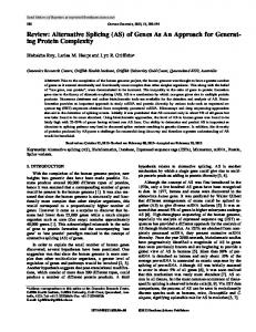
The modern view of gene expression is that DNA is transcribed into RNA containing introns and exons (called a ‘primary transcript’), and then the introns are spliced out to form a final RNA transcript which is translated into protein. Alternative splicing (AS) is a process in higher eucaryotes whereby various exons also can be spliced out, producing different RNAs (called isoforms) that can code for different proteins. AS is often tissue-dependent, so that one gene can have different tissue-dependent functions. As revealed by genome sequencing projects, apparently more complex metazoan organisms (e.g. humans) have a similar number of protein coding genes as much simpler organisms (e.g. nematodes), but AS is thought to be a major factor contributing to additional complexity in metazoans. Although there are many anecdotal, albeit well-studied, examples supporting such a view, the full extent and complexity of AS has yet to be determined [2]. As shown in Figure 1, AS can occur in different ways and the number of potential isoforms within a gene is typically quite large. In a gene with n exons, a simple analysis indicates that there are 2n − 1 possible isoforms. A relatively small number of these are expected to occur in actual tissues, but even so, compiling a genome-wide tissue-specific library of isoforms using the traditional full-length transcript (cDNA) sequencing approach is not currently feasible. There is a much larger number of transcript sub-sequence (EST) data available (200-500nt from either end of a transcript) and indeed most AS events were first discovered by mining EST databases. However, EST data does not accurately reflect tissue-dependent expression and it is biased toward the ends of transcripts. Microarray have recently been used to carry out quantitative AS studies under different physiological and pathological conditions, and to discover novel AS events. Most recently, next generation sequencing (NGS), which can generate large numbers of more uniformly-distributed transcript subsequences, has been proposed as an alternative (e.g., the Solexa system generates millions of reads about 35nt long within a day). The above technologies produce noisy data, so analyzing the many potential complex tissue-dependent AS patterns is a challenging problem. A recent review of computational methods [3] reveals that most available methods can provide only a non-quantitative analysis. For a small number of quantitative methods, the number and structure of AS isoforms has to be known in advance. More recently, the SPACE algorithm [1] based on non-negative matrix factorization (NMF) has overcome some of these limitations and appears to be able to infer both the number and structure of AS isoforms when the total number of AS isoforms is small. We describe a method that does not rely on assumptions about the number or structure of the underlying AS isoforms, but infers the frequency of different possible exon-exon junctions among AS isoforms, using microarray data. While the output of the algorithm does not identify exactly which of the exponential number of potential isoforms are expressed (only the impractical full-transcript sequencing method can do that), it does provide estimates of

PSI-Group Technical Report TR 2008– 01

University of Toronto

(a)

(b)

(c)

(d)

1

(e)

1

Constitutive exons

2 2

Alternative exons

Figure 1: Common types of AS: (a) cassette AS; (b) 5’ AS; (c) 3’ AS; (d) intron retention AS; (e) mutually exclusive AS. AS can also occur at the ends of a transcript (not shown). More complicated AS can arise from different combinations of the basic types at different exons in the same gene. local splicing event frequencies that are consistent across each gene. We present results on microarray data, but our model can be modified for use with other technologies, such as nextgeneration sequencing.

2

A Bayesian model of multi-event alternative splicing

Our model can be applied to different types of AS data. The data we used was obtained by extensively mining existing mouse and human EST and cDNA databases and established a procedure to map them to the corresponding genomic sequences and identify exons and splice junctions. With reference to popular gene annotation pipelines (Ensembl and UCSC), a comprehensive set of exons for a subset of genes of our interest was obtained. The model described here accounts for exon skipping (types (a) & (e) in Fig. 1), which is the most common category and constitutes most of the known, functional examples of AS. It does not account for alternative start and stop (polyadenylation) and assumes transcription always starts from the first exon and ends at the last exon. To account for skipping of the first or last exon, dummy exons can be included at the beginning and end of the transcript, which are never skipped. In fact, the model can be extended to account for all other types of AS in a straightforward fashion. For a gene with N exons, our model takes as input a microarray measurement for each exon (determined from a ‘body probe’) plus a microarray measurement for every possible exon-exon junction (determined from a ‘junction probe’). yi,j is the measurement for the exon i - exon j junction probe (i < j), whereas yi,i is the body probe measurement for exon i. For tissue t, the set of measurements Yt can be thought of as an upper-triangular matrix. The total number of measurements for such a gene is N + N (N − 1)/2, and our dataset consists of measurements for thousands of genes. Microarrays were designed to probe all exons and possible exon junctions when the number of exons in a gene is small, but for genes with many exons, we adopted a sliding window approach, where splicing junction probes are designed between an upstream exon and up to W downstream exons. Here, we are assuming that functional AS very rarely skips a large number of exons. At the whole-gene level, we define the following joint probability distribution over all

2

PSI-Group Technical Report TR 2008– 01

University of Toronto

observed and hidden variables in a microarray experiment: p(B, C, O, X1:T , Y1:T ) = p(B)p(C)p(O)

T Y t=1

p(Xt )

T Y

p(Yt | B, C, O, Xt ),

(1)

t=1

where B is a set of microarray probe binding affinities, Y is the set of microarray measurements and X is the set of true exon and exon junction abundances to be estimated. C accounts for cross-hybridization signals (e.g., a junction probe may stick to a molecule missing one of the exons, because 1/2 of the probe will match). O contains binary indicators that account for outlier probe measurements caused by fingerprints on the microarray, etc. p(Yt | B, C, O, Xt ) is the measurement model while p(B), p(C), p(O) and p(Xt ) are prior distributions incorporating (often weak) biological knowledge.

2.1 Microarray measurement model Similar to other analytical chemistry technology, the measurement error of a microarray probe intensity consists of a multiplicative component as well as an additive one [5]. The measured t = b xt ew + u, where b expression level is yi,j i,j is the tissue-independent probe binding i,j i,j t affinity and xi,j is the true (unknown) tissue-dependent RNA abundance for that probe. w and u are normally distributed and account for multiplicative and additive noise (w is zero mean but u may not be). A two-component noise model is quite inconvenient to work with in practice, but if the data is first normalized using variance-stabilizing normalization (VSN) [4]1 , the above exprest = arsinh(b xt ) + v, where v is assumed to be standard normally dission simplifies to yi,j i,j i,j tributed. The original multiplicative and additive noise components have been merged into a single component in the arsinh domain. We expect there to be significant cross-hybridization, i.e., hybridization of transcripts to probes that do not closely match. In particular, either half of every junction probe will match up with a corresponding exon even if the other exon is not part of the isoform. To account for cross-hybridization, we extend the above model as follows, for junction probes i 6= j: t = arsinh(b xt + c xt + d xt ) + v. The coefficients c and d (represented by C above) yi,j i,j i,j i i,i j j,j account for the degree of cross-hybridization and are inferred from the data. Note that the level of cross-hybridization is approximated as being the same for all probes matching with an exon i. t will not fit the model, because of experimental Sometimes a microarray measurement yi,j artifacts or an unexpected biological process. We use a binary variable oti,j to indicate whether (o = 0) or not (o = 1) the measurement is an outlier. If it is an outlier, the measurement noise is assumed to be quite large, with variance σ02 set equal to the data set variance. Otherwise, the measurement noise is assumed to take on the smaller value σ12 , which is inferred. The measurement model is p(Yt | B, C, O, Xt ) =

N Y

t N (yi,i ; arsinh(bi,i xti,i ), σo2i,i )·

i=1

Y

t N (yi,j ; arsinh(bi,j xti,j + ci xti,i + dj xtj,j ), σo2i,j ),

(2)

i 1, i−1 ³ ´ X p(xi,i |x1,i , . . . , xi−1,i ) = δ xi,i − xk,i , (5) k=1 2

Since the number of molecules (people) we are interested in is huge, we will assume these counts are real numbers.

4

PSI-Group Technical Report TR 2008– 01

University of Toronto

which enforces that the number of people visiting booth i equals the sum of the number of people arriving at booth i from all previous booths. For N > j > i, we have j−1 X

p(xi,j |xi,i , . . . , xi,j−1 ) = 0, if xi,j > xi,i −

xi,k ,

(6)

k=i+1

which enforces that the number of people going from i to j is upper-bounded by the number of people visiting i minus the sum of people that went from i to k where k < j. In fact, xi,j P can only depend on the difference xi,i − j−1 k=i+1 xi,k , which is the number of people that could possibly enter booth j. Define j−1 X zi,j = xi,i − xi,k . (7) k=i+1

Then, we can express p(xi,j |xi,i , . . . , xi,j−1 ) concisely as follows:   f (xi,j /zi,j ) zi,j p(xi,j |zi,j ) =  0

0 ≤ xi,j ≤ zi,j ,

(8)

otherwise,

where f can be any (user-defined) valid distribution on [0, 1], and the factor 1/zi,j is a Jacobian that spreads that distribution over the interval [0, zi,j ]. For i < N , we have N −1 h X ¢i ¡ p(xi,N |xi,i , xi,i+1 , . . . , xi,N −1 ) = δ xi,N − xi,i − xi,j

(9)

j=i+1

to make sure that all the people eventually leave the food fair via the exit. We use a beta distribution for the pdf p(xij |zij ): p(xij |zij ) =

Beta(xij /zij ; αij , βij ) . zij

(10)

If we further restrict the beta distribution parameters αij , βij to be independent of i, j, then {xi,i+1 , ..., xi,N } is the (truncated) stick-breaking construction of the Chinese restaurant (Dirichlet) process [6], while {xi,i+1 , xi,i+1 ∪ xi+1,i+2 , ..., xi,i+1 ∪ · · · ∪ xN −1,N } corresponds to the (truncated) stick-breaking construction of the Indian buffet (beta) process [8]. In our AS application, a beta prior with α = β = 0.5 is used to reflect the prior knowledge that exons are more likely to be completely included or excluded at each splicing step.

2.4 Identifiability If there were no noise, the extra information provided by the exon balance constraints would enable exact estimation of the unkown abundances, if there were enough tissue samples (and variability across tissue samples) so that the binding affinities and cross-hybridization levels could be estimated. This is in contrast to most previous microarray applications where mRNA/cDNA abundances measured by different probes either are deemed to be not quantitatively comparable or have to be compared under unjustified assumptions on the probe binding affinities. For a gene with N exons, N (N + 1)/2 probes need to be designed for exon bodies and all possible splice junctions. Under noise-free measurement conditions and ignoring cross-hybridization, the microarray measurement equation simply becomes t yi,j = bi,j xti,j ,

5

(11)

PSI-Group Technical Report TR 2008– 01

University of Toronto

where x’s can be exactly determined from the measurement once b’s are known. Therefore, the exon balance equations can be used to solve b’s by substituting x’s with (y/b)’s. For an N -exon gene measured under T different conditions, there are 2(N −1)T equations with N (N +1)/2−1 unknowns (“ − 1” is due to a common scaling factor). A necessary condition to have unique solutions for b is thus 2(N − 1)T ≥ N (N + 1)/2 − 1, (12) which gives T ≥ (N + 2)/4.

(13)

In practice, we will need more samples to offset noise, cross hybridization and the fact that AS is sparse. Another property exhibited by (13) is that the larger the gene, the more independent samples are needed to resolve B and X. However, if we adopt the sliding window probe design strategy described previously and assume that AS won’t happen outside of the window, such a dependency is reduced, leading to a number of independent samples for a sliding window size W of T ≥ 2W , which also allows cross-hybridization modeling for the exon junction probes.

3

Inference using MCMC

Here, we consider how to sample the ‘food fair process’ {xi,j } using MCMC. Suppose you would like to perturb xi,j , the number of people going from booth i to j. To maintain the constraints along i, you also need to adjust either the number of people at booth i, or the number of people going from i to at least one other booth; both can be expressed as xi,n . Similarly, you also need to adjust either the number of people at j, or the number of people arriving at j from at least one other booth; both can be expressed as xm,j . To achieve minimum number of adjustments, you could adjust xm,n accordingly and close the loop. Viewing X as an upper-triangular matrix, this will give us a “box” shape sampler that adjust four x’s at once with one degree of freedom. Based on such an intuition, we can construct the following Metropolis-Hastings sampler: • Systematically or randomly choose a boxes with four x’s, whose current values are denoted by x[i,j,m,n] . • The single degree of freedom can be viewed as a hyperplane-terminating line in a 4dimensional space with all x’s constrained to be positive. Randomly perturb the current state, e.g.by sampling from a truncated Gaussian centered at x[i,j,m,n] , to get proposed values x0[i,j,m,n] for all four x’s on the box. • Compute the acceptance ratio a: a=

p(x0[i,j,m,n] )p(y[i,j,m,n] |x0[i,j,m,n] )q(x[i,j,m,n] |x0[i,j,m,n] ) p(x[i,j,m,n] )p(y[i,j,m,n] |x[i,j,m,n] )q(x0[i,j,m,n] |x[i,j,m,n] )

,

(14)

where q accounts for the asymmetry of the truncated Gaussian proposal distribution. More specifically, a simple box that can be used for sampling is a 2 × 2 square containing xi,j , xi,j+1 , xi+1,j and xi+1,j+1 . We could choose these systematically by starting from the first row at x1,2 , moving from left to right (x1,3 , . . . , x1,N −1 ) at each row, and then moving down one row after another (x2,3 , x3,4 , . . .) until we finally reach xN −2,N −1 . Such a sweep will allow us to perturb all elements of X except x1,1 and xN,N (which will be treated specially later on). To sample these four points while maintaining the exon balance constraint, we need to have x0i,j + x0i,j+1 = xi,j + xi,j+1 , x0i,j + x0i+1,j = xi,j + xi+1,j , x0i+1,j + x0i+1,j+1 = xi+1,j + 6

PSI-Group Technical Report TR 2008– 01

University of Toronto

xi+1,j+1 , x0i,j+1 + x0i+1,j+1 = xi,j+1 + xi+1,j+1 . if none of them are on the diagonal, where x0 and x represent the new and old values of these points respectively. If xi+1,j is on the diagonal, then x0i,j + x0i,j+1 = xi,j + xi,j+1 , x0i,j − x0i+1,j = xi,j − xi+1,j , x0i+1,j − x0i+1,j+1 = xi+1,j − xi+1,j+1 x0i,j+1 + x0i+1,j+1 = xi,j+1 + xi+1,j+1 . Define ∆ ≡ x0i,j − xi,j to represent the change of x between consecutive samplings. In order to satisfy the nonnegative constraint of x, i.e., xi,j ≥ 0 for all i, j, the valid range of ∆ is ∆min = − min(xi,j , xi+1,j+1 ), ∆max = min(xi+1,j , xi,j+1 ), if xi+1,j is not on the diagonal, and ∆min = − min(xi,j , xi+1,j , xi+1,j+1 ), ∆max = xi,j+1 , if it is. The sampler for this 2 × 2 square involves sampling ∆ from a truncated Gaussian centered at 0 and bounded by ∆min and ∆max , computing new values x0 of the four points from ∆, and calculating the acceptance ratio accordingly. The above MCMC sampling strategy will not change x1,1 or xN,N , which are equal and represent the total count. When it is necessary to sample x1,1 (and xN,N ), we can first sample a random variable r from some distribution (e.g., log-normal with parameter µ = 0) and use it as a scaling factor to obtain new proposal values x0 from the product r · x, for all elements of the upper triangular matrix. Other hidden variables (b, c and d) are sampled independently respecting their bounds.

4

Results and analysis

A key component of our algorithm is the box sampler for exon abundances. Since it sequentially perturbs 2 × 2 local squares, a potential weakness is that long range changes may not propagate well through these local moves, e.g., what if AS skips a relatively large number of exons while the initial configuration is that all exons are included. We test this with simulation data while fixing all other hidden variables, and an example is shown in Figure 2 (a)-(e), where probe intensities and exon abundances are displayed as Hinton graphs. It can be observed that the algorithm performs reasonably well for this artificial example of a 4 exon skipping event with the presence of a moderate amount of noise (mostly appear as multiplicative noise changing the size of the square relative to the true abundance while the additive noise is invisible in this scale). Starting from an all inclusive initialization, the sample means virtually converges to the true abundances after about 200,000 iterations. In practice, however, we expect this kind of large skipping events to be rare and we have observed that the sampler converges much quicker to more probable configurations without these events by extensive simulation. Figure 2 (f) shows a typical example for the convergence of hidden variables, where we have simulated a 6-exon gene with 3 underlying AS isoforms differentially expressed in 8 tissues, with the presence of a moderate amount of noise and cross hybridization effect. A state of the art quantitative AS analysis method is GenASAP [7], which is specialized in analyzing cassette AS events and output the ratio between two isoforms as AS exclusion levels. Although our method is designed to work on a whole gene level, it can nonetheless analyze such a simple case. We have run our algorithm and GenASAP on a mouse array probing 3,707 cassette AS events across 33 tissues, and also performed RT-PCR3 for a subset of 37 events across 26 tissues. We compare the AS exclusion level predictions from our method and GenASAP to RT-PCR, and also to a naive method by simply computing the ratio between exon body probes (BPR). The correlation on AS exclusion level predictions summarized in the following table shows that our method compares favorably to GenASAP, while the naive BPR method performs poorly due to variation of probe binding affinity and noise in the measurement. Ours vs RT-PCR GenASAP vs RT-PCR BPR vs RT-PCR Ours vs GenASAP correlation 0.72 0.68 0.47 0.81 3

RT-PCR is a laborious experimental technique that can be used to study AS quantitatively but only one event and one tissue at a time.

7

PSI-Group Technical Report TR 2008– 01

True Exon Abundance

University of Toronto

−log(p) vs iteration

Initial Exon Abundace

1

1

2

2

3

3

4

4

5

5

6

6

7

4000

3000

2000

1000

7 1

2

3

4 (a)

5

6

7

1

2

3

4

5

6

7

0

(c)

Measured probe intensity

Estimated Exon Abundace

2

3

3

800

4

4

600

5

5

400

6

6

7

7 4 (b)

5

6

7

4

6 5

−log(p) vs iteration

2

3

(e)

1200

1

2

2

x 10

1

1

0

1000

200 1

2

3

4 (d)

5

6

7

0

0

500

1000 (f)

Figure 2: (a)-(e) simulation on a 4 exon skipping event where probe binding affinities are fixed to be the same with no cross hybridization effect added; (f) convergence of hidden variables displayed as − log(p) vs iteration for a 6 exon, 8 tissue simulation.

8

PSI-Group Technical Report TR 2008– 01

brain 1 2 3 4 5 6 7 8 9 10

University of Toronto

heart 1 2 3 4 5 6 7 8 9 10

1 2 3 4 5 6 7 8 9 10 (a)

1 2 3 4 5 6 7 8 9 10

heart 1 2 3 4 5 6 7 8 9 10

1 2 3 4 5 6 7 8 9 10 (d)

1 2 3 4 5 6 7 8 9 10 (c)

(b)

brain 1 2 3 4 5 6 7 8 9 10

liver 1 2 3 4 5 6 7 8 9 10

liver 1 2 3 4 5 6 7 8 9 10

1 2 3 4 5 6 7 8 9 10 (e)

1 2 3 4 5 6 7 8 9 10 (f)

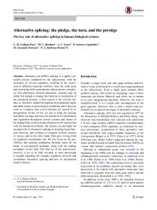
Figure 3: Data analysis of a human gene Hs.523550 shown as Hinton graphs: (a)-(c) probe intensity measurement (black boxes indicate no measurement); (d)-(e) estimated exon abundance. We have recently acquired data from our custom microarrays on 54 normal human tissues and an example of using our algorithm to analyze a gene is shown in Figure 3. For clarity of display, only 3 out of the 54 tissues analyzed are shown. Our method is able to remove most of noise in the raw data while also discover that exons 2 & 3 can be alternatively skipped, as supported by previous EST data. Interestingly, we also predicate that exons 8 & 9 can be skipped in some tissues such as liver. Novel predictions such as this are being verified and studied by biological experiments.

5

Conclusions and discussions

We introduced an MCMC procedure that infers tissue-dependent abundances of multiple splicing events in the same gene, binding affinities and cross-hybridization levels using noisy microarray measurements as input. Simulations have demonstrated the effectiveness of our method and initial, promising results have been obtained on real biological data. Besides working to obtain biologically significant results, we are also adapting the newly available SPACE algorithm to our data to perform further comparisons and possibly combine the strengths of two approaches. It should be noted that the core of our model, i.e., the exon balance constraints, is generally applicable whenever both exon and exon junction measurements are available. As a result, we are also extending the method to NGS data by modifying the noise model and using domain specific priors for that technology.

9

PSI-Group Technical Report TR 2008– 01

University of Toronto

References [1] M. A. Anton, D. Gorostiaga, E. Guruceaga, V. Segura, P. Carmona-Saez, A. PascualMontano, R. Pio, L. M. Montuenga, and A. Rubio. SPACE: an algorithm to predict and quantify alternatively spliced isoforms using microarrays. Genome Biology, 9(2):R46, 2008. [2] B. J. Blencowe. Alternative splicing: New insights from global analysis. Cell, 126:37–47, 2006. [3] M. Cuperlovic-Culf, N. Belacel, A. S. Culf, and R. J. Ouellette. Data analysis of alternative splicing microarrays. Drug Discovery Today, 11(21/22):983–990, 2006. ¨ [4] W. Huber, A. von Heydebreck, H. Sueltmann, A. Poustka, and M. Vingron. Variance stabilization applied to microarray data calibration and to the quantification of differential expression. Bioinformatics, 18(Suppl. 1):S96–S104, 2002. [5] D. M. Rocke and B. Durbin. A model for measurement error for gene expression arrays. J Comput Biol, 8(6):557–569, 2001. [6] J. Sethuraman. A constructive definition of Dirichlet priors. Statistica Sinica, 4:639–650, 1994. [7] O. Shai, Q. D. Morris, B. J. Blencowe, and B. J. Frey. Inferring global levels of alternative splicing isoforms using a generative model of microarray data. Bioinformatics, 22(5):606– 613, 2006. ¨ ur, ¨ and Z. Ghahramani. Stick-breaking construction for the Indian buffet [8] Y. W. Teh, D. Gor process. In Proceedings of the International Conference on Artificial Intelligence and Statistics, volume 11, 2007.

10