International Journal of Transportation Science and Technology · vol. 1 · no. 3 · 2012 – pages 229 – 246
229
Inferring Pavement Properties using an Embedded Accelerometer Eyal Levenberg Technion - Israel Institute of Technology, Technion City, Haifa 32000, Israel
[email protected]
ABSTRACT A high-end single-axis inertial sensor, capable of detecting minute accelerations, was embedded in an asphalt pavement system. A vehicle of known dimensions and overall weight was driven along a straight line, passing near the sensor’s embedment location at constant speed. Measured accelerations were analyzed as means to infer the pavement layer properties. For this purpose, instead of double integrating the accelerometer data to arrive at deflections, the raw measurements were first smoothed and then matched against computed accelerations. Vehicle speed and weight distribution between front and rear axles were also backcalculated. The paper describes the experimental details, analysis method, and results.
1. INTRODUCTION Pavements are layered systems made of geomaterials designed and built to serve as physical transportation infrastructure. Knowledge of the pristine layer properties and their evolution throughout the life of the system is valuable to the pavement engineers [1, 2], as it enables better construction quality control, monitoring of structural health, and improved performance forecastability. Study of layer properties in the laboratory is both challenging and difficult for three main reasons: (i) the necessity to recreate the prevailing in situ conditions such as stress levels, moisture contents, etc., (ii) the need for destructive field sampling to obtain specimens, and (iii) the unavoidable interruption of traffic flow. It is envisioned that future pavements will include sensory gear for detecting, measuring, recording, and even analyzing various mechanical responses. For such ‘smart pavements’ the aforementioned problems may be circumvented by deducing the sought after layer properties in-place. This can be potentially performed by way of inverse analysis making use of data collected under ordinary service conditions without interrupting traffic flow and without destructive sampling. In addition, the sensors may
230
Inferring Pavement Properties using an Embedded Accelerometer
also be used to capture traffic characteristics such as travel speeds, wheel loads, axle weight distributions, and vehicle dimensions. Traditionally, pavement engineers have been concerned with stresses, strains, and deflections resulting from moving loads. Perhaps for this reason the current commercial offering of pavement sensors targets such responses [3-5]. While these perform adequately in research applications, it is hard to envision their widespread usage due to high price tag and installation difficulties; moreover, the vast majority of available sensors require electric wiring that are vulnerable and pose limits on embedment options. Accelerometers are inertial sensors designed to detect velocity rates at the point of measurement in one, two, or three perpendicular directions. Despite the popularity these sensors enjoy in fields such as biology, medical, seismology, machinery, automotive, and consumer electronics, the usage of accelerometers in pavement systems (apart from seismic pavement testing) has received only limited attention [6-8]. Especially for a medium composed of geomaterials, measuring acceleration of a point in the system is fundamentally superior, i.e., more closely related to the physical reality, as compared to stresses and strains which are essentially mathematical abstracts. In recent years, due to increased commercial demand, accelerometer technology has improved in terms of sensitivity, frequency response, power consumption, physical size, and ruggedness of packaging; at the same time, end-user unit costs continued to drop. Consequently, inertial sensors should be considered as natural candidates to serve as (wireless) pavement sensors. In the work of Ryynänen et al. [6] a low-volume asphalt road, comprised of a thin asphaltic layer covering a granular structure, was instrumented with sensors - including displacement transducers and near-surface accelerometers. Loading experiments were conducted whereby a truck of known weight and dimensions was driven over the gauge array along different paths and speeds. Measured accelerations were double-integrated with respect to time to arrive at deflections. It is reported that calculation corrections were necessary (and applied) to offset artificial data drift. Even so, discrepancy was seen between deflections calculated from accelerations and the measurements of the displacement transducers. A layered elastic pavement model was used to match the deflections; the derived moduli, however, seemed unrealistic. As proclaimed in the paper (but not pursued), a possible remedy could be the introduction of nonlinearity into the model. In the work of Arraigada et al. [7, 8], accelerometers were implanted in two full scale asphalt pavements along with deflectometers. Measured accelerations generated by moving loads were double integrated in an attempt to calculate deflections. Difficulties were reported in arriving at deflections because of the sensitivity of the integration operation to signal noise and drift. Arraigada et al. suggested and applied a spline-based correction in an effort to alleviate the problem. This resulted in ‘reasonable qualitative correlation’ between direct deflection measurements and deflections calculated from double-integrating accelerations. In addition, difficulty was mentioned in dealing with slow-moving loads. The problem of obtaining displacement information from accelerations has been
International Journal of Transportation Science and Technology · vol. 1 · no. 3 · 2012
231
dealt with in numerous studies [9-13]. The first and trivial concern lies within the numerical process, which is only approximating the continuous core signal to be integrated. The resulting errors may be improved (minimized) by increasing the sampling rate and selecting appropriate integration method. The main problem however, is that of integrating a signal contaminated with noise and drift [14, 15], which leads to an output that has a root mean square value that increases with integration time even in the absence of any motion of the sensor. For velocities, errors are a function of the duration of the signal; for displacements, errors are a function of the square of the duration of the signal. This means that both amplitude and timing affect the error budget with early observations in the acceleration history record making a higher impact on the calculation results. Attempts to tackle the latter problem include rules for offsetting, smoothing, and filtering the raw data before integration [16-18]. Such approaches received limited success since in many applications the signal of interest and the noise have very close bands of frequency. At this time it is accepted that reliable displacements cannot be extracted from inertial sensors without other aided sensors or prior knowledge of motion characteristics. This study is part of a larger research effort intended to accommodate the ‘smart pavement’ vision. In this connection, previous studies by the author had focused on backcalculating layer properties using an embedded array of stain and stress gauges [1923]. These studies showed the potential of using implanted sensors to infer pavement attributes nondestructively, and without interrupting traffic flow. They tackled the challenges of forward modeling, formulation of the multi-criterion inverse problem, and explored a range of modeling complexities, including: isotropic elasticity, anisotropic elasticity, and linear viscoelasticity. The current study pursues the ability of inferring pavement properties using data registered by embedded inertial sensors. At this time, only a single sensor is used and hence a rudimentary pavement model is applied. An attempt is also included to backcalculate some traffic characteristics. 2. THE SENSOR The inertial sensor used in this study was model KB12VD manufactured by Metra Meß (Germany). It is a single-axis piezoelectric accelerometer designed for measuring low intensity vibrations. It has a relatively narrow measuring range of ±0.6 µgn accompanied by very high sensitivity of the order of 1 µgn; it responds linearly (±3 dB) in the frequency range of 0.08 to 260 Hz. A 24 bit high-accuracy data acquisition (DAQ) module, model NI 9234 manufactured by National Instruments, specifically designed for making measurements from integrated electronic piezoelectric (IEPE) sensors, was used to ‘drive’ and sample the KB12VD. A two-meter long cable was used for connecting the accelerometer to the NI 9234 unit, while the DAQ module itself was connected via USB to a computer. Referring to Figure 1, a protective enclosure shaped as ‘cage’ was designed for the accelerometer. It is composed of three aluminum disks (numbered sequentially in the figure), each 80 mm in diameter and 10 mm in thickness, and three narrow hollow cylinders, each 50 mm long. The underside of the accelerometer is firmly attached (screwed) to the middle disk (No. 2) while its circumference and top part are untouched.
232
Inferring Pavement Properties using an Embedded Accelerometer
A 50 mm gap between the top disk (No. 1) and middle disk (No. 2) is maintained using three long screws running through the hollow cylinders and through three holes in the middle disk (No. 2). These screws can only be tightened against the bottom disk (No. 3), resulting in a rigid structure. When performing measurements, the bottom disk (No. 3) is initially connected to a surface on (or in) the system being monitored; this can be done using glue or other means. The sensor ‘cage’ can then be fixed to the system by tightening the three screws. After taking measurements, by simple release of the screws, the sensor (along with disks 1 and 2), may be disconnected for storage or moved to another measurement location; the bottom disk remains in-place, glued to the system providing means for reattaching the sensor at a later time.
Figure 1.
View of ‘caged’ accelerometer
As means of elementary validation, the KB12VD was attached to the piston of a servo-hydraulic loading frame. A sinusoidal movement was applied to the piston with a frequency of 10 Hz and amplitude of 0.5 mm. Under such conditions, the sensor should measure a sinusoidal acceleration with an identical frequency (of 10 Hz) and amplitude of about 200,000 µgn. Because the load frame and sensor had separate data acquisition systems, data logging from the sensor began first (at t=10) and terminated last, employing a sampling rate of about 1652 Hz for a total duration of 18 seconds. In between, from t=7.3 to t=10.3 seconds, 300 sinusoidal cycles were executed by the piston (logged separately). Figure 2 presents a close view of the sensor readings, spanning half a second, beginning at t=8.5 seconds; measured accelerations are depicted in the figure using
International Journal of Transportation Science and Technology · vol. 1 · no. 3 · 2012
233
circular markers. Due to vibrations of the piston, which are typical for servo hydraulic machines, the raw data is ‘noisy’; nonetheless, a clear sinusoidal pattern can be identified with the correct frequency of 10 Hz. The smooth solid line seen passing through the markers was obtained by fitting a pure harmonic curve to the measurements using a leastsquares approach. The amplitude of the fitted curve is about 200,000 µgn (as anticipated), indicating that both the sensor and DAQ module are functioning correctly.
Figure 2.
Accelerometer measurements of a servo-hydraulic piston executing sinusoidal movements.
3. FIELD EXPERIMENT 3.1 Setup A field experiment was performed using the KB12VD; it basically consisted of embedding the sensor in an asphalt pavement, and driving a vehicle of known weight and dimensions close to the embedment location. A plan view of the tested scenario is depicted in Figure 3, showing the accelerometer as a crossed circle, and providing a schematic representation of the vehicle. For reference purposes, a right-handed Cartesian coordinate system is included in the figure with its origin located on the surface such that: (i) the X-axis coincides with the travel direction of the vehicle; (ii) the Y-axis is perpendicular to the travel direction; and (iii) the Z-axis (not shown) points downward into the pavement system, asserting that positive vertical acceleration means downward. The vehicle used was a Toyota Hiace van - model LXH12L-SBSRXW (1999), having a total weight of 18.5 kN (i.e., relatively lightweight) and dimensions as shown.
234
Inferring Pavement Properties using an Embedded Accelerometer
The four automobile tires are numbered counter clockwise starting from the left front side. The offset distance between the sensor and a line connecting the centers of tires 1 and 2 is denoted by y0.
Figure 3.
Schematic plan view of the field experiment setup.
The experiment was conducted over a low volume road with a relatively thin structural section comprised of a 100 mm thick asphalt concrete layer covering an aggregate base course layer with a thickness of about 120 mm. Auger drilling and visual inspection showed that the subgrade in the area is composed of lean clay with a moisture content that is slightly below the plastic limit; the top 200 mm of the subgrade contained 20% by volume of chalky gravel inclusions. A dual mass (8 kg) dynamic cone penetratrometer (DCP) with a 60 degree cone apex angle [24] was utilized to estimate the shear resistance of the pavement layers near the test location. After core drilling the asphaltic layer, the DCP test commenced from the top of the aggregate base course down to a depth of 1,000 mm from the surface. The penetration results are displayed in Figure 4, in which blow count is plotted vs. depth of penetration; layering of the pavement system is shown on the right hand side. As indicated by the chart, penetration rates (PRs) are almost four times higher for material deeper than 450 mm (i.e., the upper 450 mm are more resistant to penetration). Approximate California bearing ratio values appearing in the figure were related to PRs based on [25]. In order to install the accelerometer, the asphaltic layer was first core-drilled to a depth of 80 mm and disk No. 3 (refer to Figure 1) was fixed to the bottom of the blind hole with a two-component Epoxy glue. Then after, the accelerometer enclosure (with the sensor) was screwed to the base plate and connected via the DAQ module to a portable computer. The top and sides of the sensor (and ‘cage’) were covered with a piece of cotton fabric as shield from direct wind effects. Additionally, a Tekscan ‘map’ was placed on the pavement surface near the accelerometer. This ‘map’ is a thin pressure-sensitive sheet that can measure the load distribution within the tire footprint [26]. Specifically, map #3150 was used, which is rectangular in shape and contains 2188 individual load sensitive points arranged in a matrix that is 436 mm long and 369 mm wide. The experimental setup was such that tires 1 and 2 (refer to Figure 3) drove
International Journal of Transportation Science and Technology · vol. 1 · no. 3 · 2012
235
directly over the Tekscan map as the vehicle was passing next to the accelerometer. The map readings were scanned at a rate of 100 Hz, allowing direct measurement of the offset distance yo (refer to Figure 3) and providing validation information regarding the speed and intensity of the applied load.
Figure 4.
Dynamic cone penetrometer test results and pavement system layering.
3.2 Raw Data The field experiment contained several Toyota Hiace passes; the passes differed from one another in terms of offset distance yo, vehicle speed, and ambient temperature conditions. Presented and analyzed hereafter are data from a single pass, performed under a surrounding temperature of about 23 degrees Celsius. Based on the Tekscan sensor readings, the offset distance for this single pass was 570 mm, the vehicle was traveling at a speed of 5880 mm/s (i.e., about 21 km/h), and the front axle carried 52% of the total weight of the van. Figure 5 presents acceleration data collected by the sensor during the experiment. Four charts are included, each showing vertical acceleration on the ordinate vs. time on the abscissa. The sampled readings, at a rate of 2048 Hz, are shown using solid circular markers; for visual clarity, they are connected with straight thin line segments. The top left chart presents the entire experiment, it contains 60,000 points spanning almost 30 seconds during which the vehicle was approaching the accelerometer, passing by it, and moving further away. While the location of the vehicle relative to the sensor in the Xaxis direction (refer to Figure 3) was not monitored, it is graphically clear that the
236
Inferring Pavement Properties using an Embedded Accelerometer
movement was detected by the sensor between about t=22 and t=25 seconds. The top right chart provides a closer view of the acceleration data during these three seconds; no clear/distinct pattern can be recognized, as it is masked by other vibration sources, e.g., car engine mechanical and acoustical vibrations. The two bottom charts in Figure 5 provide a close view of data recorded before the moving load was apparently detected by the KB12VD. The bottom left chart contains 213 = 8,192 data points, between t=6 and t=10 seconds; the bottom right chart shows a closer view, covering a 0.1 second interval beginning at t=8.0 (204 data points). A band of noisy readings can be seen in these two charts, having a ‘thickness’ of about 120 µgn and mean level (or bias) of about -40 µgn (i.e., different from zero). These noisy accelerations are two orders of magnitude larger than the sensor sensitivity.
Figure 5.
Raw vertical acceleration readings.
A discrete Fourier transform was applied to the four seconds of noisy data in the bottom left chart of Figure 5 (after subtracting the mean from the measurements). The results of the transformation are shown in Figure 6 over a frequency range of 0.1 to 1000 Hz (note the double logarithmic scale). The average magnitude level is represented by the horizontal dashed line seen crossing the chart. Magnitudes larger than the average occur at low frequencies (less than 1.0 Hz), between 30 and 100 Hz, and also between 300 and 500 Hz (which is outside the linear sensor range). These vibrations most likely describe so-called ‘cultural noise’ originating from distant traffic and machinery. As the
International Journal of Transportation Science and Technology · vol. 1 · no. 3 · 2012
237
tested area was surrounded by buildings and pine trees, wind turbulence around topography irregularities, and the coupling of tree motion to the ground also contributed to the detected ambient noise [27-30]. It is also probable that radio frequency interferences, intercepted by the sensor and its cable, were also contributing to the observed noise.
Figure 6.
Fourier analysis of ambient noise detected by accelerometer.
4. ANALYSIS 4.1 Methodology and forward calculations In general terms, the analysis of the measured accelerations aims first and foremost at inferring the pavement layer properties by way of inverse analysis. The method herein proposed for achieving this objective consists of three steps: (i) simulating the moving vehicle in a pavement model and computing the acceleration history at the sensor location; (ii) smoothing the measured acceleration history to expose and ‘separate’ the effects of the moving load from other vibration sources; and (iii) matching the computations against the smoothed measurements by adjusting the model parameters at which point the derived layer properties are assumed to best represent the in situ pavement condition at the time of measurement. As described in what follows, the last two steps are intertwined because it was deemed necessary to utilize the pavement model for providing guidance and control over the smoothing efforts. A relatively simple mechanical model is selected to represent the pavement, presuming it is a stratified half-space comprised of two fully bonded linear elastic
238
Inferring Pavement Properties using an Embedded Accelerometer
layers, each isotropic, homogeneous and weightless. The top layer represents the structure, with a finite thickness h1 and elastic properties E1 and v1 (Young’s modulus and Poisson’s ratio respectively); the underlying half-space represents the subgrade, with elastic properties E2 and v2. The vehicle is simulated with four loaded regions representing tire-pavement contact; these are positioned relative to each other based on the van dimensions (Figure 3). Each region is circular, with a diameter of 190 mm equal to the tire width. In the model, horizontal shear forces are disregarded, and it is assumed that every tire exerts uniform vertical stress to the surface of the top layer; the intensity of this stress is simply calculated as half the axle weight divided by the area of contact. Movement at a constant speed along the X-axis (refer to Figure 3) is simulated quasi-statically (i.e., neglecting inertia effects) by applying the four tire loads in different locations relative to the origin of the coordinate system. Vertical displacements at the sensor location were first calculated instead of accelerations with the layered elastic program ELLEA1 [23]. A set of 62 computations was executed by the program for a two-layered system loaded by a single wheel. Each computation gave the vertical displacement at a different radial distance from the load centroid for a point embedded at a depth of 80 mm from the surface; radial distances ranged (non-uniformly) between zero and 50,000 mm. From this displacement set, a much larger and denser set, consisting of more than 8,000 displacements (each corresponding to a different radial distance within the abovementioned range), was generated using cubic spline interpolation. This denser set allowed simulating the deflection history of the sensor due to the moving vehicle at a given speed, for a period of 10 seconds at 0.005 second intervals. The effect of the four tires was obtained by way of superposition - exploiting linearity. Vertical accelerations at the sensor location where then computed from the deflection history by numerical differentiation with respect to time. Finally, additional interpolation step was applied, this time to the computed accelerations, in order to generate three seconds of closely spaced data points matching the sampling rate of the measurements. Before performing the inverse analysis, data smoothing was applied to the measured accelerations. Numerous methods are offered by the technical literature for this purpose, e.g., least-squares [31, 32], regularization [33, 34], signal filtering techniques [35-37], etc. Each method has its advantages and disadvantages, and each has user-changeable parameters that influence the outcome. The smoothing procedure selected herein (discussed below) is based on an iterative process proposed in [38]; it is relatively simple to program, fast to compute, and does not mandate evenly sampled data - although not an issue herein. Denoting Accn(0) as the measured acceleration at time tn where n is an integer ranging between 1 and the total number of points NT (i.e., 60,000), a single smoothing iteration consists of: (i) connecting all data points by straight lines; (ii) locating the center point (0) of each interval with coordinates tn+0.5 = 0.5tn + 0.5tn+1 and Acc(0) n+0.5 = 0.5Accn + (0) 0.5Acc n+1; (iii) connecting by straight lines this new set of ‘center points’; and (iv) finding new acceleration values Accn(1) corresponding to the original tn’s (n=1..NT) by linear interpolation over each interval. The resulting acceleration set is slightly smoother compared to the original ‘raw data’ and can be used as a starting point for another
International Journal of Transportation Science and Technology · vol. 1 · no. 3 · 2012
239
iteration. Accn(i) denotes a smoothed acceleration value after i iterations corresponding to time tn. The only ‘user-selectable’ parameter in this method is the number of iterations. The following expression enumerates the difference or ‘fitting error’ between a set of raw accelerations and the same set after i smoothing iterations. It is based on accumulating the squared differences between the two datasets:
Fitting_Error(i) =
1 N 2 − N1
n= N2
∑ ( Acc
(i ) n
− Accn( 0 )
n = N1
)
2
(1)
in which N1 and N2 are ‘place holders’ identifying the subset within the entire dataset (i.e., N1