In‡ation Projections in In‡ation Targeting: To Forecast or to Simulate? Michal Skorepa,¤Viktor Kotlan Monetary Policy Department Czech National Bank Prague September 2002
Abstract In‡ation targeting is a regime based to a great extent on in‡ation projections. Central banks, however, devote surprisingly little attention to some important issues connected with the projection. There are some nontrivial choices that need to be made on three distinct levels: construction, decision making and communication. One of the most important choices relates to the treatment of central bank’s behaviour within the projection. We …rst di¤erentiate between a forecast (most likely picture of the future) and a simulation (picture of the future if the behaviour of one or more agents is adjusted) and then discuss the pros and cons of using the two types of projections on the three mentioned levels.
Our thanks for useful comments received at the outset of the writing of this paper go to Nicoletta Batini, Jaromír Beneš, Aaron Drew, Mojmír Hampl, Douglas Laxton and Kateµrina Šmídková. The views expressed are those of the authors, and not necessarily those of the Czech National Bank. ¤ The corresponding author: Michal Skorepa, Monetary Policy Division, CNB, Na prikope 28, Prague 1, CZ-11503, Czech Republic,
[email protected].
1
1
Introduction and basic terms
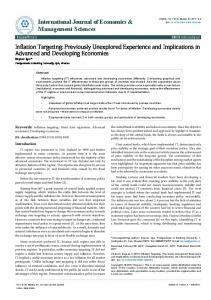
In‡ation projections are in the centre of today’s monetary policy conduct. This is true not only for direct in‡ation targeting (often labelled in‡ation forecast targeting after Svensson (1997)), but also for other less explicit ‡exible-exchangerate regimes. And yet, central banks devote surprisingly little attention to some important issues related to projections. This paper aims to …ll in this gap by discussing some non-trivial choices that need to be made regarding in‡ation projections on three distinct levels: construction, decision-making and communication. We focus on the very heart of in‡ation projections – on the treatment of the central bank’s behaviour within the projection. Before we discuss the pros and cons of the alternative treatments, we need to devote our attention to the terminology. Any outlook into the future will be referred to as a “projection”. The distinction between two particular types of projection, namely a “forecast” and a “simulation”, will be central for this paper. By a “forecast” we will mean a projection that tries to draw the most likely picture of the future in all respects - i.e., using the most likely scenario of each exogenous variable, at each time period selecting the most likely reaction of each economic agent represented in the model, taking the most likely value of each coe¢cient, etc. This is how the term “forecast” is understood generally. In central-banking circles, this “forecast” is often referred to as “unconditional forecast” to distinguish it from a “conditional forecast”, which is a purposeful attempt to draw not simply the most likely picture of the future, but the most likely picture of the future if one of the agents behaves in a speci…c (not necessarily the most likely) way - speci…cally, if the central bank does not change the level of its interest rate throughout the forecasted period of time (see, e.g., Tarkka and Mayes (1998)). Any such projection (not just the no-change one) in which the forecaster “forces” a given agent to behave in a speci…c (not necessarily the most likely) way, will be called a “simulation” here (sometimes the term “experiment” is used as well). This terminology is illustrated in Figure 1.
2
projection
forecast („unconditional forecast“)
simulation
assumed constant rate („conditional forecast“)
RF or assumed nonconstant rate
Figure1: Basic types of projections The labels “conditional” and “unconditional” are potentially misleading because in reality, all projections are conditional on some assumptions, while the above use of the terms restricts the terminology just to one special type of conditionality. That is why we think that the terminology introduced here is preferable, apart from being more natural. In practice, when building a model on which to base a forecast, the reactions of the central bank are usually generated by a reaction function. This is a speci…c equation in which the value of the decision variable (typically the central bank’s interest rate) is determined by past, current or expected values of various variables in a way that - at least in the opinion of the model builders approximates the decision-making criteria of the actual central bank’s decisionmakers (from now on simply “the board”). In simulations, the trajectory of the board’s decisions may be determined directly by the model builder without any modelling or it may be generated by inserting various reaction functions into the predictive model.1 Clearly enough, there is usually just one forecast at each point of time (except cases like multiple equilibria) because just one picture of the future is usually the most likely one. On the other hand, there can be as many simulations as we can devise trajectories of the central bank’s future decisions. At …rst sight, it may seem straightforward that obtaining and using a standard forecast, i.e., the most likely picture of the future is preferable and that it makes little sense to weaken the predictive value of the projection by making it a simulation, i.e., by assuming that one of the agents will behave in a way that is not necessarily the most likely one (so that the overall result of the projection may not be the most likely outlook). 1 With regard to exchange rate, note that we consider the short-term interest rate to be the only central bank’s instrument, think of the exchange rate as being determined within the model and abstract from possible FX interventions. If interventions were to be considered as a standard policy instrument, we would have to enrich the discussion of simulations accordingly.
3
Central bankers, however, do …nd simulations useful, as indicated in Table 1. The reason is that such simulations are one way how to “evaluate”,(as Lucas (1976) puts it) alternative policies.
Projection used for decision making
Published trajectory of
Simulation assumes
Examples of countries
constant IR and ER
Australia, Hungary
Simulation
IR
Sweden
ER constant as assumed
constant as assumed
yearly averages of EER
UK
constant as assumed
quarterly average of EER at end of forecast period
Canada
none
none
Czech Republic
basic shape verbally
basic shape verbally
New Zealand
quarterly averages of 3M IR
half-year averages of EER rounded to integers
constant IR
Forecast
Note: The table is based on the central banks‘ various publications available in Spring 2002. Since then, the practice at some of the banks may have changed. Abbreviations: IR = central bank‘s interest rate, ER = exchange rate, EER = effective exchange rate.
Table 1: Use and communication of projections at some in‡ation-targeting central banks
The goal of the present paper is to identify advantages and disadvantages of the use of forecasts and simulations in the areas of projection construction, monetary policy decision-making and projection communication. The rest of the paper is organised accordingly: sections 2 to 4 compare the two types of projection at these three levels and section 5 concludes and o¤ers some policy recommendations for the Czech National Bank.
2
Construction of simulations and forecasts
To avoid any misunderstanding, we emphasise that since the most common di¤erence between forecasts and simulations as used in central banking practice is their treatment of the central bank, the comparison in this and in the following sections will be based on this di¤erence alone. Problems that are common to both these types of projection will be suppressed here.2 In this section we want to compare simulations and forecasts in terms of their construction. 2 An example of problems common to both types of projections is that the board is composed of several decision-makers who may often have di¤erent preferences, information sources, perception of the situation, etc., so that wherever a judgment of „the board“ is required, we have to be ready to solve the delicate task of aggregating several di¤erent opinions.
4
2.1
Simulations and the Lucas critique
In reality, all agents quite naturally expect that all other agents will in the future behave the most likely way. If one of the agents, namely the central bank, then in fact behaves (as the simulation generally assumes) in a way that was not judged as the most likely, this will surprise the other agents and falsify to some extent their expectations. As a result, individual agents may change to some extent their perception of the central bank’s behaviour and, consequently, they may change their own behaviour. The simulation, in order to be the “most likely picture of the future, given that the central bank behaves in the assumed way”, has to predict all these changes and their implications for the behaviour of all agents. The simulation will be able to predict the changes the better, the closer the underlying predictive model will be to the ideal of a fully micro-founded, disaggregated, structural model of the economy. In practice, it is almost impossible to build the ideal, fully structural, micromodels where the decision-making of each agent is explicitly modelled. Instead, actual predictive models are of a more or less reduced, aggregated form and the structure of and coe¢cient values in many of their relationships are based on regularities observed in the past when all agents including the central bank behaved roughly the most likely, expected way. And so while an unexpected behaviour of the central bank would not necessitate a change in the structure and values of the fully structural models, it may imply the need to change structure and/or values in the reduced-form relationships. This is one interpretation of the Lucas (1976) critique: the assumption that the central bank behaves in an unexpected way may imply a need to change the structure and/or coe¢cient values in the rest of the predictive model. And here lies the key problem of simulations: it is very di¢cult to guess exactly how the structure and/or coe¢cient values should change. Indeed, it is so di¢cult that model builders often do not take these changes into account. The decision not to incorporate these changes, however, causes the results of the simulation to deviate from what they should be, namely the most likely picture of the future given that the central banks behaves in the assumed way. The simulation thus contains an error. We will call such an erroneous simulation “degenerated”. Of course, if the central bank’s trajectory assumed in the simulation is not far from the bank’s most likely trajectory (so that the simulation is close to a standard forecast), then the implied changes that should be done in the rest of the model may be negligible and also the error of the simulation may be negligible. An example may be a simulation where we want to see what would happen if a needed rate cut is postponed by the central bank by three months. Given all sorts of uncertainties in the practice of monetary policy, this delay may not surprise agents in the economy very much so that the existing forecasting model may remain roughly valid and the simulation may be close to a forecast. The less realistic is the assumed central bank’s trajectory, the more significant will be the implied changes and the larger will be the error, that is, the more degenerated the simulation will be. For example, consider a period of 5
rapidly growing domestic demand when a sharp rate hike is in order. In such a situation, a simple simulation with constant interest rates for the next several quarters may– if the above mentioned Lucas critique is not accounted for – show a picture that is very far from what would really happen if the central bank actually followed the no-change trajectory. Unfortunately, there is no way to assess the simulation’s error, to assess the degree of its degeneration. To sum up, on the level of construction, the main problem with simulations is that they may be more or less degenerated and therefore provide a more or less misleading information. On the other hand, by constructing simulations, we avoid a problem that has to be dealt with when constructing a forecast: the di¢culty of identifying the most likely reaction function of the central bank. In simulations, either no reaction function of the central bank is identi…ed and simply various trajectories of its future behaviour are assumed, or various reaction functions are inserted into the predictive model without trying to earmark the most likely one.
2.2
Forecasts and the speci…cation of the central bank’s reaction function
The construction of a forecast, on the other hand, is impossible without identifying the most likely reaction function. As with any economic agent’s reaction function, this is not an easy task. There are several approaches that come to mind. One approach, which we will call the “loss function” approach, is based on determining the loss function of the board and then transforming it through model optimisation into the “true”, or most likely reaction function. A second approach, which we will call the “shock response” approach, rests in presenting the board members with simulations showing model responses to di¤erent shocks under various arbitrarily chosen reaction functions. Another approach, which may be called the “estimation” approach, aims at extracting the reaction function from the board’s past decisions. We will now discuss these three approaches in more detail. In the …rst step of the “loss function approach”, the board members are shown a table with a few key variables and they …ll in relative weights they assign to (the stabilisation of) the given variables in comparison with the others. In the second step, the model builder constructs a loss function based on the answers. The last step is to transform the loss function through model optimisation into the most likely reaction function. This approach combines a very crude questionnaire part in the …rst two steps with a rigorous model optimisation in the last step. Although this way of identifying the central bank’s reaction function may seem attractive at …rst sight, the problem is that it depends heavily on the assumption that the board members are able (with the help of the model builder in the second step) to formalise their preferences and able to do it in a non-biased way. Moreover, the optimal reaction function that comes out of this approach is often too complex to be useful as a guide for policy discussions. The “shock response” approach is similar to the one above but it combines, in a sense, all the three steps into one. To begin, the model builder designs a 6
realistic reaction function, runs the model under various shocks (demand, supply, risk premium and other shocks) and then presents the board members with the responses of the key variables to the shocks. If the board members feel convenient with the response paths of the variables, the reaction function is chosen as the most likely one. If they are not satis…ed, the assumed reaction function is changed, responses to the same shocks under the new reaction function are presented to the board and assessed. This iterative process goes on until the board accepts the reactions, which means that the most likely reaction function has been found. Unfortunately, this is a rather demanding and time-consuming process. Moreover, since the individual iterations are simulations, they are subject to the “degeneration” problem described above, unless the model builder is able to adjust the rest of the model so that it captures the changes in the behaviour of the other agents corresponding to the changed reaction function of the central bank. The “estimation approach” builds on past data. This is not easy to do properly since there is a potentially strong simultaneity bias at play. As this is a common problem, we will now describe the way it may arise in more detail. If we believe the central bank responds in a forward-looking manner to ‡uctuations in future in‡ation and future real economic activity, it may occur natural at …rst sight to try to estimate the relationship between the central bank’s interest rate at a moment in time and later actual …gures on in‡ation, real economic activity, etc. But in practice, interest rates react in a forward-looking manner to shocks that would otherwise push in‡ation away from the target. This means that, if policy is successful, past data will show that interest rates have ‡uctuated, while in‡ation has stayed more or less at the target level.3 To sum up: if policy reacts to anticipated shocks that are later unobservable from actual data, then the estimation of the central bank’s reaction function from past data is impossible. Box: The simultaneity bias and the consumption of vitamins To further illustrate the simultaneity bias, let’s move from economics to the area of preventive healthcare. Suppose one attempts to evaluate the impact of vitamins’ consumption on one’s health-state by comparing the amount of consumed vitamins and the evolution of one’s health. Since it is relatively easier to catch a cold in the winter than in the summer, one’s consumption of vitamins will likely be higher in the winter than in the summer. While the consumption of vitamins ‡uctuates throughout the di¤erent seasons of a year, one’s health state should ideally stay unchanged. If one pre-emptively consumes a lot of vitamins in the winter and does not catch a cold, we would hardly conclude that there is no relationship between the consumption of vitamins and the health-state. Likewise, monetary policy doses interest rate changes (vitamins) according to expected evolution of economic cycle and various anticipated shocks (health). If the relationship between interest rates and in‡ation or GDP is 3 In this paper, when talking of ful…lling the central bank‘s in‡ation target, we implicitly mean a balanced ful…lment of the in‡ation target and any other targets the central bank may have (minimising the output gap, etc.).
7
not recognisable from past data, it can simply mean that the pre-emptive policy (cure) was successful and the state of the economy (of the patient) did not change.
Is there any way to avoid the simultaneity bias in the estimation of the central bank’s reaction function? It may seem that the way to proceed rests in realising that the board’s decisions are based on forecasts, not actual future data, and that the forecasts are always based on past and actual data. Reacting to forecasts then basically means reacting to a combination of past and actual data. One may therefore try to obtain the reaction function by constructing and estimating a VAR-type-relationships between interest rates and several other variables such as in‡ation, domestic and foreign output gap, exchange rate, etc. Some central banks may even have a time series of simulations of future development (usually based on the constant interest rate assumption) at their disposal. In that case, we could directly estimate the relationship between the divergence of the simulation from the target as an independent variable and (lagged) interest rates as a dependent variable. Although these two approaches seem attractive, one should be careful since they too are subject to some simultaneity bias. The reason is that concurrent and even past values of in‡ation and other variables already incorporate expectations about the future, including future interest rate policy. The di¢culties central banks have when trying to come up with the most likely reaction function may seem paradoxical, given that it is their own reaction function. In fact, however, the central bank’s model builders face similar di¢culties when modelling (through reaction functions or otherwise) the behaviour of the other agents in the economy. The model behaviour of the central bank is special only in the sense that the actual central bank has a choice: either to ask its model builders to model its own most likely reaction function (i.e., to construct a forecast) or to ask them to construct simulations instead of a forecast. If the …rst option is chosen, then one (or preferably a combination) of the above-mentioned or other approaches must be attempted, bearing in mind the limitations.
3
Use of simulations and forecasts the monetary policy decision-making
in
As in the previous section, we will start with simulations and we will - unless noted otherwise - assume away the problem of degeneration. The reason for the attractiveness of simulations in the area of decision-making is clear - they enable the central bank to do what Lucas (1976) calls „policy evaluation“. That is, they show what the results would be (in terms of in‡ation, output etc.) if the central bank follows alternative future interest rate trajectories. Speci…cally in in‡ation targeting, once we compare the simulation with the in‡ation target, we may get an idea about the direction in which the central bank‘s interest rate
8
trajectory assumed in the simulation needs to be adjusted, in order to bring in‡ation closer to the target at the policy horizon. Unfortunately, the policy advice a simulation gives is incomplete: it is qualitative (direction) but not quantitative (extent). The information about how much to adjust the trajectory has to be obtained elsewhere. For example, we can analyse the monetary policy transmission mechanism in order to get an idea of the sensitivity of in‡ation in various future horizons to a unitary change in the central bank‘s current interest rate. To do this with any reliability is, however, a very di¢cult task. Moreover, the sensitivity of in‡ation on the central bank’s interest rate is likely to depend on the particular shock in question. Another possibility how to supply the quantitative advice is to construct and present to the board members a fan of simulations, showing the future development of the economy assuming several alternative trajectories of the central bank‘s interest rate. The board members then simply select the simulation whose results they like most, ask for values of the interest rate trajectory upon which the selected simulation is based and set the actual interest rate in accord with the starting value of that trajectory. The process can even be iterative - the board selects a simulation out of a fan of simulations, the sta¤ prepares and presents a fan composed of a few variations of the selected simulation, the board selects again, etc. Note a link to a forecast: after a su¢ciently high number of iterations, the simulation selected at the end should be very close to a forecast. Understandably, the problem with the “fan approach” is that it is a rather time-consuming process. The link between a fan of simulations and a forecast clearly shows the basic di¤erence between simulations and a forecast: those who construct simulations do not need to understand the preferences of the board members into any depth. These preferences come to play only at the moment the board members select the simulation they like most - i.e., only after the simulations are …nished and lie on the table of the board members. On the other hand, to construct a forecast, the sta¤ need to understand the board members‘ preferences well because these preferences have to come to play already at the moment the forecast is being constructed - i.e., before it gets on the table of the board members. The last issue we want to discuss in connection with the use of simulations in monetary policy decision-making, is the assumption of unchanged central bank‘s interest rate. Theoretically, simulations can assume various trajectories of the central bank‘s interest rate, from completely ‡at trajectories (unchanged central bank’s interest rate) to very complex shapes. In practice, however, central banks (e. g., Bank of England, Sveriges Riksbank, Magyar Nemzeti Bank) tend to prefer the ‡at extreme, that is, trajectories which assume no change in the interest rate. Board members at these central banks apparently see advantages of the constant central bank‘s interest rate assumption over other, more complex assumptions. Maybe they think that such a simulation is easiest to grasp and work with because a constant nominal interest rate keeps the impact of monetary policy on the economy constant (which is not true, if in‡ation expectations change and if it is the real interest rate that matters). Or maybe the board 9
members think that such an assumption is just a naturally obvious choice for a simulation. Or they appreciate the extreme simplicity of the trajectory as showing most blatantly to the public that the projection is a mere simulation, not an actual forecast of the central bank‘s future interest rate trajectory (for a discussion of the publication of this trajectory, see section 4). On the other hand, the constant interest rate assumption has a disadvantage to which we alluded already in section 2 and which we have assumed away in this section so far. The more unrealistic (vis-´r-vis current and anticipated economic circumstances) is the no-change trajectory that the sta¤ is required to assume in the simulations, the higher is the risk of degeneration of the simulation. Less degeneration might be achieved by taking more complex and more realistic trajectories. Let’s now brie‡y discuss monetary policy decision-making based on forecasts. An integral part of the forecast is a trajectory of future central bank’s interest rates. The board is thus directly suggested what decision trajectory it should follow in order to ful…l its in‡ation target. Although this suggestion might also be arrived at through a series of simulations, the construction of a forecast seems to be a more straightforward way. The high “…xed costs” connected with arriving at the most likely reaction function are compensated by very low “variable costs” which in the case of simulations may get quite high (see section 2). The problem with the suggested trajectory of the central bank’s interest rate is that the board members may feel obliged to accept it, they may feel “locked up in it”. In reality, however, they do not have to agree to the suggestion. For example, they may attach various additional risks to the basic forecast presented, their preferences may have changed from the time the reaction function was determined, etc.
4
Use of simulations and forecasts in central bank’s communication
Today, many central banks strive for a high degree of transparency. Many central bankers would also agree that publishing in‡ation projections is a key characteristic of transparency. And yet, if you ask a central banker for reasons to publish in‡ation projections, you may get a long hesitation and unclear answer that “everybody else does that and it is necessary for transparency reasons”.
4.1
Why to publish the in‡ation projection?
Since the form of publishing a projection must re‡ect its goals, let us start by discussing the reasons to publish a projection. We see two basic reasons. The …rst is that the projection can anchor expectations in times when the central bank expects to miss its in‡ation target so that the target in itself ceases to serve as the usual expectation anchor. There are situations (mainly supply shocks) when it may be economically legitimate and substantiated for the central bank 10
not to react (or to react only partially) to an expectation that its in‡ation target will be missed. These situations arise with a particularly high frequency and severity in small open economies exposed to frequent external shocks.4 In such situations the public may ask what they should expect, given that in‡ation will diverge from the target; the central bank can answer by publishing its projection. In the other case, i.e., when the projection signals that the in‡ation target will be ful…lled, the projection’s publication won’t bring much added value in terms of anchoring expectations, but it won’t do any harm in this area either. Obviously, the only type of projection suitable for this purpose is the currently valid forecast, where by „currently valid“ we mean a forecast which incorporates also the board‘s latest decision. This implies that if the board makes its decision on the basis of a forecast but the decision is not as forecasted, then a new forecast has to be constructed to incorporate the actual decision (which may take some time). A simulation - or even a forecast that does not incorporate the board‘s last decision - is not a suitable expectation anchor as it is not the central bank‘s best guess about the future. The second reason for the central bank to publish its projection is that the projection can serve as an explanation of the decision that the board has just taken. This explanation can have two forms. First, it can show what unwelcome results would probably ensue if the decision were not taken. A simulation as well as a forecast not including the decision being explained, will serve well. However, only the appropriate direction, not the appropriate extent of the decision to be taken is shown. This form thus allows only a qualitative assessment of the appropriateness of the decision actually taken. Second, it can be shown what welcome results will probably ensue thanks to the decision having been taken. This form of explanation is informationally richer as it shows that the decision actually taken was the appropriate one both qualitatively and quantitatively, that is, in terms of both direction and extent. For this form, only the currently valid forecast can be used.
4.2
Publishing the trajectory of interest rate and other variables consistent with the forecast
The above analysis of the motivation for communicating the central bank’s projection into the future seem to imply that overall, a forecast may be preferable to a simulation. Several arguments can, however, be raised against publishing a forecast. We will mention two, calling them the “commitment argument” and the “destabilisation argument”. The “commitment argument” (e.g., Goodhart (2001)) runs as follows. If the in‡ation forecast is to be believed as credible, the agents need to know its key properties and assumptions. If the central bank is an important player in the economy, then the path of the central bank’s interest rate is an important component of the forecast and it should be made public. The problem is that 4 These central banks sometimes even explicitly state their in‡ation target may not be ful…lled under speci…c types of shocks. This arrangement is then referred to as „escape clauses“.
11
agents in the economy may view the trajectory as a commitment of the central bank to keep its future interest rate at the published level. Of course, there are reasons why the trajectory should not be viewed in this way. First, the board members may have other decision inputs beside the forecast, they may - as mentioned in the previous section - attach various additional risks to the forecast, etc.5 Moreover, the trajectory, just as the whole forecast, is based on today’s information, so that any new piece of information obtained later may potentially modify the forecast and thus the future part of the central bank’s interest rate trajectory. These reasons, however, may be di¢cult to communicate to the general public and therefore the perception of commitment may remain very strong. The second argument against publishing a forecast, the “destabilisation argument”, is more economic in nature. The argument is that if the central bank is perceived to produce high quality forecasts and if it publishes a forecasted trajectory of certain …nancial variables, namely the short-term market interest rates and the exchange rate, this may have a highly destabilising e¤ect on the respective markets. More speci…cally, if the central bank publishes a forecast showing an exchange rate appreciation, this forecast may concentrate market expectations at the forecasted level of appreciation as well as decrease future uncertainty. This concentration of expectations and reduction in uncertainty may then cause the appreciation to occur much faster. An easy pragmatic solution to this problem is to publish the forecasted trajectory of the exchange rate with some fuzziness added, e.g., by publishing the forecasted trajectory of an e¤ective exchange rate without publishing the weights in the basket of currencies used to calculate it (see Table 1). While we think that the destabilisation argument may be true for the exchange rate, we believe the same argument does not hold in the case of shortterm market interest rates. The reason is that the central bank is usually able to control current short-term market interest rates at the forecasted level and the market is aware of this ability of the central bank. This has a useful implication: the published forecast of the central bank’s interest rate trajectory may help concentrate market expectations of future short-term market interest rates at the level suggested by the central bank’s forecast, thus concentrating, through the term structure, today’s long-term interest rates at a level consistent with the forecast. To conclude this section, there are arguments both for and against publishing the interest rate trajectory consistent with the given forecast. Fortunately, a compromise solution similar to the exchange rate case may be found. Namely, the central bank may choose how explicit it is while communicating the future interest rate trajectory. The Reserve Bank of New Zealand, for instance, publishes both a chart and a table of future quarterly averages of the 90-day interest rate. As an example of a less explicit publication, the Czech National Bank describes in simple words the direction in which interest rates consistent 5 In other words, publishing a forecast with the interest rate trajectory does not necessarily mean a „policy bias“ in the sense of, for example, the Fed’s “bias announcements“ published between May 1999 and January 2000.
12
with the presented forecast will move in the future.6
5
Policy recommendations National Bank
for
the
Czech
As we saw, the choice between simulations and forecasts has several dimensions and it is certainly not a straightforward choice. Before opting for one of the two approaches or switching between them, speci…c circumstances at the given central bank have to be considered - the sophistication of the modelling apparatus available, the length and quality of the data series that can be used, the degree of risk of the public misunderstanding the communicated message, etc. Of course, the ultimate choice will to a large extent depend on which of the two options will seem more “user-friendly” to the board members. In what follows, we will brie‡y o¤er some policy recommendations for the practice of the Czech National Bank (CNB). In the area of terminology, our recommendation is that, both internally and in its communication, the CNB should avoid the terms “conditional forecast” and “unconditional forecast” and prefer the terms “simulation” and “forecast”. In the area of projection construction, the sta¤ as well as the board should be aware of the degeneration problem whenever simulations are being used. Suggestions to build simulations on extremely unlikely assumed decision trajectories in order “to see the impact more clearly” may result in simulations that give a very misleading message. This problem may arise especially in the so called “policy experiments” conducted during the preparation of a new forecast. Related to the construction of projections is also the point that when identifying the most likely reaction function, one should preferably use the shock response approach together with the VAR-based estimation approach and avoid the loss function approach. In its decision making as well as communication, the CNB has recently switched to using forecasts. We want to emphasise two issues in the communication area, which - in our opinion - deserve a continued attention of the CNB’s sta¤ and board. First, if the actual decision taken by the board does not correspond to the forecasted trajectory of the central bank’s interest rate, the forecast is no longer valid and therefore cannot be used to anchor in‡ation expectations. In these cases the costs of producing a new forecast immediately after the decision need to be weighted against the potential harm caused by publishing such an obsolete forecast, admitting it is obsolete and waiting for the regular construction and publication of a new forecast. Second, as for publishing the interest rates consistent with the forecast, we suggest to continue with the current practice of verbal description of the 6 This may re‡ect the fact that in the case of the RBNZ, there is a single decision-maker, the governor of the RBNZ, whose (most likely) reaction function is mapped onto the forecast, whereas in the case of the CNB, there are seven decision-makers whose „average“ reaction function enters the forecast.
13
trajectory. After some time the accrued experience with this regime should be analysed and a more explicit approach may be adopted if no obstacles are found.
14
References Goodhart, C. A. E. (2001): Monetary transmission lags and the formulation of the policy decision on interest rates. FRB of St. Louis Review, July/August, pp. 165-186. Lucas, R. E. (1976): Econometric policy evaluation: A critique. In Brunner, K., Meltzer, A. H. (eds): The Phillips Curve and the Labor Markets, supplementary series to the Journal of Monetary Economics, pp. 19-46. Svensson, L. E. O. (1997): In‡ation Forecast Targeting: Implementing and Monitoring In‡ation Targets. European Economic Review, 41, pp. 1111-1146. Tarkka, J., Mayes, D. G. (1999): The Value of Publishing O¢cial Central Bank Forecasts. Bank of Finland Discussion Papers, No. 22/99.
15