Jul 19, 2011 - ... probability that indegree is d. We show that the quantity that characterizes the dynamic be-. arXiv:1107.3792v1 [cond-mat.dis-nn] 19 Jul 2011 ...
Influence and Dynamic Behavior in Random Boolean Networks C. Seshadhri, Yevgeniy Vorobeychik, Jackson R. Mayo, Robert C. Armstrong, and Joseph R. Ruthruff
arXiv:1107.3792v1 [cond-mat.dis-nn] 19 Jul 2011
Sandia National Laboratories, P.O. Box 969, Livermore, California 94551-0969, USA We present a rigorous mathematical framework for analyzing dynamics of a broad class of Boolean network models. We use this framework to provide the first formal proof of many of the standard critical transition results in Boolean network analysis, and offer analogous characterizations for novel classes of random Boolean networks. We precisely connect the short-run dynamic behavior of a Boolean network to the average influence of the transfer functions. We show that some of the assumptions traditionally made in the more common mean-field analysis of Boolean networks do not hold in general. For example, we offer some evidence that imbalance, or expected internal inhomogeneity, of transfer functions is a crucial feature that tends to drive quiescent behavior far more strongly than previously observed.
Introduction. Complex systems can usually be represented as a network of interdependent functional units. Boolean networks were proposed by Kauffman as models of genetic regulatory networks [1, 2] and have received considerable attention across several scientific disciplines. They model a variety of complex phenomena, particularly in theoretical biology and physics [3–8]. A Boolean network N with n nodes can be described by a directed graph G = (V, E) and a set of transfer functions. We use V and E to denote the sets of nodes and edges respectively, and denote the indegree of node i by Ki . Each node i is assigned a Ki -ary Boolean function fi : {−1, +1}Ki → {−1, +1}, termed transfer function. If the state of node i at time t is xi (t), its state at time t + 1 is described by xi (t + 1) = fi (xi1 (t), . . . , xiKi (t)). The state of N at time t is just the vector (x1 (t), x2 (t), . . . , xn (t)). Boolean networks are studied by positing a distribution of graph topologies and Boolean functions from which independent random draws are made. We denote the distribution of transfer functions by T . An early observation was that when the indegree of a network is fixed at K and each transfer function is chosen uniformly randomly from the set of all K-input possibilities, the network dynamics undergo a critical transition at K = 2, such that for K < 2 the network behavior is quiescent and small perturbations die out, while for K > 2 it exhibits chaotic features [2]. This result has been generalized to non-homogeneous distributions of transfer functions, when the output bit is set to 1 with probability p (called bias) independently for every possible input string [9]. The resulting critical boundary is described by the equation 2K p(1− p) = 1. All analysis of Boolean networks to date uses mean-field approximations, an annealed approximation [9], simulation studies [1, 7], or combinations of these, to understand the dynamic behavior. Many previous studies rely solely on shortrun characteristics (e.g., Derrida plots that consider only a very short, often only a single-step, horizon [4, 5, 7]) and extrapolate to understand long-term dynamics. Hamming distance between Boolean network states that diverges exponentially over time for small perturbations to initial state suggests sensitivity to initial conditions typically associated with chaotic dynamical systems. Nonetheless, the connection be-
tween short-run and long-run sensitivity is not a foregone conclusion [10] and remains an open question. We provide a formal mathematical framework to analyze the behavior of Booleam networks over a logarithmic (in the size of the graph) number of discrete time steps, and give conditions for exponential divergence in Hamming distance in terms of the indegree distribution and influence of transfer functions in T . Assumptions. We assume that the Boolean network N is constructed as follows. First, we specify an indegree distribution D with a maximum possible indegree Kmax , and for each node i independently draw its indegree Ki ∼ D. We then construct G by choosing each of the Ki neighbors of every node i uniformly at random from all n nodes. Next, for each node i we independently choose a Ki -input transfer function according to T . We assume that the family T has either of the following properties: • Full independence: Each entry in the truth table of a transfer function is i.i.d., or • Balanced on average: Transfer functions drawn from T have, on average, an equal number of +1 and −1 output entries in the truth table. Formally, Pr f ,x [ f (x) = +1] = 1/2, where Pr f ,x denotes the probability of an event when f is drawn from T , and input x for f is chosen uniformly at random. Influence. The notion of influence of variables on Boolean functions was defined by Kahn et al. [11] and introduced to the study of Boolean networks by Shmulevich and Kauffman [4]. The influence of input i on a Boolean function f , denoted by Infi ( f ), is Infi ( f ) = Prx [ f (x) 6= f (x(i) )], where x(i) is the same as x in all coordinates except i. Given a distribution T of transfer functions, let Td denote the induced distribution over d-input transfer functions. The expected total influence under Td , denoted by I(Td ), is E f ∼Td [∑i Infi ( f )]. When Td is clear from the context we write this simply as I(d). Suppose that we have an indegree distribution where p(d) is the probability that indegree is d. We show that the quantity that characterizes the dynamic be-
2 havior of Boolean networks is I =
Kmax
∑
p(d)I(d).
d=1
Main Result. We present our main result that characterizes dynamic behavior of Boolean networks under the assumptions stated above. Define t ∗ = log n/(4 log Kmax ). The following theorem tracks the evolution of Hamming distance up to time t ∗ , starting with a small (single-bit) perturbation. We note that our theorem applies for any distribution of indegrees with a maximum bounded by Kmax , though increasing density (Kmax ) shortens the effective horizon t ∗ . Theorem 1 Choose a random Boolean network N having a random graph G with n nodes and a distribution of transfer functions T . Evolve N in parallel from a uniform random starting state x and its flip perturbation x(i) (with a uniform random i). The expected Hamming distance between the respective states of N at time t ≤ t ∗ lies in the range I t ± 1/n1/4 . The proof of this theorem is non-trivial and is provided in the supplement. It shows that the effects of flip perturbations vanish when I < 1 while perturbations diverge exponentially when I > 1. Thus, criticality of the system is equivalent to I = 1. Much of the past work assumed (or explicitly stated) that it suffices to consider the expected influence value I(K) for the mean indegree K. A direct consequence of Theorem 1 is that I(K) characterizes a critical transition iff I(d) is affine. To see this, observe that I(K) = I iff I(K) = I (∑d d p(d)) = ∑d p(d)I(d). This is true if and only if I(d) is affine. Applications. In this section we use Theorem 1 to recover most of the characterizations of critical indegree thresholds to date and prove results for new natural classes of transfer functions. We show that our assumptions are crucial in obtaining the observed results. An important step in applying the theorem is computing the quantity I(d) for a given class of transfer functions T . The following proposition (proven in the online supplement) facilitates this process. Let B d denote a d-dimensional Boolean hypercube. The edges of B d connect pairs of elements with Hamming distance 1. A function f : B d → B can be represented by labeling element x ∈ B d by f (x). An edge of B d is called f -bichromatic if one endpoint is labeled +1 and the other −1. Proposition 2 Consider a distribution Td over d-input functions. Then I(Td ) =
E f ∼Td [# f -bichromatic edges] . 2d−1
Uniform random transfer functions. We begin with the classical model of random Boolean networks in which each entry in the truth table of a transfer function is chosen to be +1 and −1 with equal probability. It has previously been observed that the critical transition occurs at mean indegree K = 2 [9]. We now demonstrate that it is a simple corollary of our theorem. First, we need to compute I(d) using Proposition 2.
In this model, the probability that an edge is f -bichromatic is exactly 1/2. Hence, I(d) = (total number of edges)/2d . Since the total number of edges (of B d ) is d2d−1 , we obtain I(d) = d/2. Notice that I(d) is linear in this case, and, consequently, considering I(K) = K/2 suffices for any distribution p(d). Applying Theorem 1 then gives us the well-known critical transition at K = 2. Transfer functions with a bias p. A simple generalization of uniform random transfer functions is to introduce a bias, that is, a probability p that an entry in the truth table is +1 (but still filling in the truth table with i.i.d. entries) [2]. In this case, the probability that an edge is f -bichromatic is 2p(1− p) and therefore I(d) = 2d p(1 − p). Since I(d) is linear, we can characterize the critical transition in this case at 2K p(1 − p) = 1 for any indegree distribution with mean K. Canalizing functions. Kauffman [2] and others have observed that since uniform random transfer functions are typically chaotic, they are unlikely to represent a distribution of transfer functions that accurately models real phenomena, such as genetic regulatory networks. Biased transfer functions only partially resolve this, as they still tend to fall easily into a chaotic regime for a rather broad range of p [6]. Empirical studies of genetic networks suggest another class of transfer functions called canalizing. A canalizing function has at least one input, i, such that there is some value of that input, vi , that determines the value of the Boolean function. Shmulevich and Kauffman [4] show heuristically that canalizing functions have I(K) = (K + 1)/4 and thus exhibit a critical transition at K = 3. We now show that this is a corollary of our theorem, using Proposition 2 to obtain I(d). To compute I(d), fix (without loss of generality) the canalizing input index to be 1 and the canalizing input and output values to +1. Consider the distribution of functions conditional on these properties. By symmetry, the expected number of bichromatic edges conditional on this is the same as the overall expectation. Hence, we can focus on choosing f from this conditional distribution. Split the hypercube B d into the (d − 1)-dimensional sub-hypercubes B 0 and B 00 such that B 0 has all inputs with x1 = +1 and B 00 has all inputs that have x1 = −1. Edges can be partitioned into three groups E 0 , E 00 , E ∗ . The set of edges E 0 (resp. E 00 ) are those that are internal to B 0 (resp. B 00 ). The set of edges E ∗ have endpoints in both B and B 0 . Note that |E 0 | = |E 00 | = (d − 1)2d−2 , and |E ∗ | = 2d−1 . Because the function is canalizing, the edges in E 0 are all f -monochromatic, and all other edges are f -bichromatic with probability 1/2. Hence, the expected number of bichromatic edges is ((d − 1)2d−2 + 2d−1 )/2 = 2d−1 (d + 1)/4. By Proposition 2, we then have I(d) = (d + 1)/4. Since this is affine in d, we can conclude that I(K) = (K + 1)/4 characterizes the short-run dynamic behavior for any indegree distribution with mean K. Threshold functions. A threshold function f (x) with d inputs has the form sgn[ f ∗ (x)] with f ∗ (x) =
1 ∑ wi xi − θ , d i≤d
3
When d is odd, bichromatic edges are those that connect the bd/2c-level to the dd/2e-level. For d even, these are the edges connecting the d/2-level to the (d/2 − 1)-level (or the (d/2 + 1)-level). In either case, the number of these edges d � is dd/2e bd/2c , giving I(d) as above. Consequently, when d = 1 or 2, I(d) = 1, while for d ≥ 3, I(d) ≥ 3/2. Thus, if a Boolean network has a fixed indegree K, it is critical for K ≤ 2 and chaotic for K > 2. Strong majority function. We now show an interesting and natural class of functions where the expected average influence goes down as the indegree d increases. Consider threshold functions where wi = 1 for all inputs i and the threshold is either θ or −θ with equal probability for some fixed θ ∈ [0, 1]. For example, when θ = 1/3, the function returns +1 iff a 2/3 majority of inputs have value +1. For this class of functions, bichromatic edges are those that connect the bd/2 + ρdc-level to the dd/2 + ρde-level, where ρ = θ /2. Thus, the expected number of bichromatic edges for a fixed d is � � d Be = (d − bd/2 − ρdc) , bd/2 + ρdc
2.5 1/5 1/6 1/7
2 Sensitivity parameter
where xi is the value of input i, wi ∈ {−1, +1} is its weight, which has a natural interpretation of an input being inhibiting (wi = −1) or excitatory (wi = +1) in regulatory networks, and θ is a real number in [−1, +1] representing an inhibiting/excitatory threshold for f . Such 2-input threshold functions have been studied by Greil and Drossel [12] and Szejka et al. [13] and are classified as biologically meaningful by Raeymaekers [14]. We now use Theorem 1 to show that random threshold functions lead to criticality for any indegree distribution. Consider T in which the value of wi for each input i, as well as θ , are chosen uniformly at random. To compute I(d), consider a threshold function with threshold θ and an edge (x, x(i) ). This edge is bichromatic exactly when the θ lies between f (x) and f (x(i) ). Note that | f ∗ (x) − f ∗ (x(i) )| = 2/d, regardless of the values w1 , . . . , wd . Since the range of θ has size 2, the probability that this happens is (2/d)/2 = 1/d. So I(d) = (# of edges)/d2d−1 = 1. Since it is independent of d, the result follows immediately by Theorem 1. Majority function. An important specific threshold function is a majority function, which has wi = 1 for all inputs i and θ = 0. Suppose T consists exclusively of majority functions. We demonstrate that the quiescence-chaos transition properties of this class are very different from those of general threshold functions. One detail that needs to be specified for T is what to do when the number of positive and negative inputs is exactly balanced. To satisfy the condition that T is balanced in expectation, we let the output be +1 or −1 with equal probability in such an instance (for a specific majority function this choice is determined, but it is randomized for any majority function generated from T ). Given this T , we now show that � � d dd/2e . I(d) = d−1 bd/2c 2
1.5
1
0.5
0 0
10
20
30
40
50
K
FIG. 1. The x-axis is K. The y-axis gives the average influence parameter I(K). We show the cases where ρ = 1/5, 1/6, 1/7. For larger ρ we reach quiescent behavior more rapidly with increasing K.
and, consequently, I(d) = Be /2d−1 . In Figure 1 we plot I(K), where K is a fixed indegree, for different values of ρ. There are two rather remarkable observations to be made about this class of transfer functions: first, the sawtooth behavior of I(K), and second, that the Boolean network actually becomes more quiescent with increasing K. To our knowledge, this is the first example in which there is no single critical transition from order to chaos, and increasing connectivity leads to greater order. We show that for d large enough, I(d) tends to 0. For convenience, assume that d is an even integer and θ d is non-integral. By � tail bounds on binomial coefficients, 2−d ∑r≥bd/2+ρdc dr < 2−cd for some constant c. (This can be proven using a Chernoff bound, such as Theorem 4.1 in [15].) Hence I(d) < 1 for large enough d, and tends to zero as d increases. We had previously noted that it is commonly assumed that I(d) is linear in d. Strong majority transfer functions feature I(d) that is clearly non-linear, and we therefore expect this assumption to be consequential. To illustrate, consider two network structures: one with a fixed K = 4, and another where the indegree distribution follows a power law with mean K = 4. Using θ = 1/3, in the former, we get I = I(K) = 1.5, while in the latter (with Kmax = 100), I = 0.79. Thus, while a fixed K yields decidedly chaotic dynamics, using a power law distribution with the same mean indegree produces quiescence. The importance of graph structure. Our results rely fundamentally on the fact that the inputs into each node are chosen independently. The fact that the size of the neighborhood at distance t grows exponentially with t is crucial for our proofs. Furthermore (for the random graphs we sample from), this neighborhood is a root directed tree, when t < t ∗ . When graphs exhibit only polynomial local growth, we do not expect chaotic dynamic behavior even when other conditions for it are met. We illustrate this point in Figure 2 (left), which compares a random network with K = 4 to a grid (a bidirectional square lattice that also has K = 4). While both initially appear to be in a chaotic regime, the Hamming distance stops diverging for a grid, but diverges exponentially in the random network. The importance of being balanced. The assumption that T is balanced is crucial. Balance has previously been noted to
(!"
:,/;9-""?@"A"&B"