Oct 14, 2009 - 044502 (2006); S.J. Chapman and G. Kozyreff, Physica. D (Amsterdam) 238 ... [22] D.J.B. Lloyd et al., SIAM J. Appl. Dyn. Syst. 7, 1049. (2008).
week ending 16 OCTOBER 2009
PHYSICAL REVIEW LETTERS
PRL 103, 164501 (2009)
Influence of Boundaries on Localized Patterns G. Kozyreff,1 P. Assemat,2 and S. J. Chapman3 1
Optique Nonline´aire The´orique, Universite´ Libre de Bruxelles (U.L.B.), CP 231, Belgium Nonlinear Physical Chemistry Unit, Universite´ Libre de Bruxelles (U.L.B.), CP 231, Belgium 3 OCIAM, Mathematical Institute, 24-29 St Giles’s, Oxford OX13LB, United Kingdom (Received 20 May 2009; published 14 October 2009)
2
We analytically study the influence of boundaries on distant localized patterns generated by a Turing instability. To this end, we use the Swift-Hohenberg model with arbitrary boundary conditions. We find that the bifurcation diagram of these localized structures generally involves four homoclinic snaking branches, rather than two for infinite or periodic domains. Second, steady localized patterns only exist at discrete locations, and only at the center of the domain if their size exceeds a critical value. Third, reducing the domain size increases the pinning range. DOI: 10.1103/PhysRevLett.103.164501
PACS numbers: 47.54.�r, 05.65.+b, 47.11.St, 89.75.Kd
Pattern formation, especially the Turing instability, is one of the principal shaping mechanisms of the macroscopic world [1]. In this context, periodic patterns of infinite extent are well understood, but localized patterns (LP) are much harder to study. Yet, their finite character makes them obviously more realistic from a physical point of view. This has motivated a very large body of research, starting perhaps with the quest of solutions having their own ‘‘natural boundaries’’ in reaction-diffusion systems [2]. Subsequently, LP have been found and studied in a wide variety of contexts where the Turing instability comes into play: chemistry [3], nonlinear cavity optics [4–7], mechanics [8–10], fluid mechanics [11,12], vegetation systems [13], electroconvection [14], and biochemistry [15]. Clearly, the underlying dynamics is universal, and it is therefore appropriate to try and understand it with a simple model. Perhaps the simplest such model is the quadratic-cubic Swift-Hohenberg equation, which often comes as a natural asymptotic reduction of more complicated models in some limit [16]. Previous studies of this equation in steady state have highlighted the peculiar bifurcation diagram associated to LP [8,17,18]. Plotting the size, or energy, of the LP as a function of the control parameter, LP are found to exist in a pinning range of parameters centered on the ‘‘Maxwell point.’’ On an infinite domain, the diagram mainly consists of two interlaced snaking curves, where each fold signals the appearance of a new peak in the LP. The two snaking curves are in addition connected by ‘‘ladder’’ branches of unstable asymmetric solutions [10,19]. This diagram has been described analytically only recently [20], when the amplitude of the pattern is small. Since then, general statements could be made about the structure of the snaking diagram even for large amplitude [21]. Recently, the snaking diagram was computed numerically for systems with two spatial dimensions [22] and was recorded experimentally both in one- and two-dimensional nonlinear optical cavities [7]. Despite the extensive research reviewed above, very little has been done in the way of a systematic investigation 0031-9007=09=103(16)=164501(4)
of boundary effects on LP. Recently, localized convection patterns were numerically studied for closed containers [23]. Existing analytical results are limited either very close to the Turing instability, i.e., to solutions that have not yet developed into a stable LP, or to patterns that fill most of the domain [24,25]. In the intermediate case, nothing is known in general. Usually, when the system is large enough, the influence of boundaries is considered negligible, and periodic boundary conditions are assumed for the sake of computational convenience. However, both of these attitudes can lead one to dangerous modeling avenues. Indeed, we will show that the presence of boundaries may strongly affect LP, even when they are far from the edges. Moreover, periodic boundary conditions produce quite distinct outcomes from what is obtained with more general boundary conditions. To demonstrate these claims, we analyze the SwiftHohenberg equation @u ¼ ru þ 3Eu2 � u3 � ð1 þ @2x Þ2 u; @t
0 < x < �; (1)
where � denotes the domain size. We make no assumption on the boundary condition, except that u be small there. In this sense, we consider solutions that are truly localized pffiffiffiffiffiffiffiffiffiffiffi within 0 < x < �. If E � 3=38, stable small amplitude patterns with unit wave number coexist with the stable homogeneous state. Focusing on this region and on steady states, we set uðx; tÞ ¼ ��fðxÞ;
r ¼ ��4 ;
(2)
and therefore study ð1 þ @2x Þ2 f þ �4 f þ 3�Ef2 þ �2 f3 ¼ 0:
(3)
Above, � fixes the amplitude of spatial oscillations and E is the main control parameter. LP exist in a narrow range of parameters described by
164501-1
E ¼ EM ð�Þ þ �E;
(4)
Ó 2009 The American Physical Society
pffiffiffiffiffiffiffiffiffiffiffi where EM ð�Þ ¼ 3=38 þ �2 E2 þ . . . is the Maxwell point and �E is a small deviation from it. EM ð�Þ was computed up to 4th order in [20] and, in particular, we have E2 � 0:534. As illustrated in Fig. 1, a LP is characterized by the distances ‘1 and ‘2 to the domain boundaries or, equivalently, by its center of mass R and size L. Our aim is to relate R and L to �E, and we shall now sketch how this can be done when � � 1. The following analysis, however, is found to give excellent qualitative and quantitative predictions, even for the moderately small value � ¼ 0:6 assumed in the numerical simulations. In order to treat the problem analytically, we need to assume that �, ‘1 , and ‘2 are all Oð1=�4 Þ. This ensures that the pattern amplitude at x ¼ 0, � is comparable to the 2 pinning force, which is Oð��4 e��=� Þ [20]. With this assumption, distinct asymptotic approximations fI , fII , fIII , and fIV of LP solutions hold in each of regions I to IV of Fig. 1. Once these approximations are obtained, the matching conditions between them lead to the bifurcation diagram. In the vicinity of x ¼ ‘1 , f is described by a front that ‘‘switches on’’ spatial oscillations. The asymptotic expression of this front is well known and given by the multiplescale expansion fII �
N�1 X n¼0
week ending 16 OCTOBER 2009
PHYSICAL REVIEW LETTERS
PRL 103, 164501 (2009)
~ þ RN ð~ ~ �n fn ð~ x; XÞ x; XÞ;
0.5 II
I
0
III
IV
0.5 0
R
1
2
FIG. 1 (color online). A numerical solution of (1) for � ¼ 0:6, � ¼ 20�, E ¼ 0:4195, and f ¼ fx ¼ 0 at x ¼ 0, �. The LP is composed of an up-switching front at x ¼ ‘1 , region II, and a down-switching front at x ¼ � � ‘2 , region III. Near the boundaries, regions I and IV, f � 1 and distinct asymptotic approximations can be derived. R is the center and L ¼ � � ‘1 � ‘2 is the size of the LP.
By the x ! � � x symmetry of (3), where � is a constant, the down-switching front in region III is given by ^ ^ XÞ; fIII ¼ fII ðx;
(7)
with x^ ¼ � � x þ ‘2 þ ’2 , X^ ¼ �2 ð� � x � ‘2 Þ. pffiffiffiffiffiffiffiffiffiffiffiffiffiffi Close to the left boundary, we set fI ¼ 19�=2 � expð��2 ‘1 =2ÞFðx; �Þ, and since ‘1 ¼ Oð1=�4 Þ, this is exponentially small in �. Hence, (3) becomes
(5)
2
ð1 þ @2x Þ2 F þ �4 F ¼ Oðe�� ‘1 =2 Þ;
where x~ ¼ x þ ‘1 þ ’1 , and X~ ¼ �2 ðx � ‘1 Þ. The leading order term in fII is given by [20] sffiffiffiffiffiffiffiffiffi ~ ~ ~ ¼ 19�ei~xþX=2 x; XÞ ð1 þ eX Þ�ð1þi�Þ=2 þ c:c:; (6) f0 ð~ 2 pffiffiffiffiffiffiffiffi where � ¼ 1= 734. As x~, X~ ! �1, (6) decreases exponentially and becomes Oð expð��2 ‘1 =2ÞÞ at the left boundary. On the other hand, the limit x~, X~ ! 1 is to the center of the LP where spatial oscillations have a uniform amplitude. The approximation (6) can be improved by computing further terms f1 ; f2 ; . . . in (5), but the resulting sum eventually diverges. By truncating it at order N where �N fN is smallest, one obtains a remainder RN that is exponentially small in �. It is this remainder that contains the information relative to the interaction between the slow and fast scales X~ and x~, as well as the deviation �E to the Maxwell point (see [20]). Presently, RN also contains terms produced by the boundaries. Some of these terms are necessary to achieve matching between the various approximations of f in regions I to IV. We omit the details here.
(8)
which is linear to a very good approximation. Solutions of (8)pare thusffi exponentials of the form expðikxÞ, where k ¼ ffiffiffiffiffiffiffiffiffiffiffiffiffiffiffi � 1 � i�2 � �ð1 � i�2 =2 þ . . .Þ. Consequently, 2
2
2
fI / e�� ‘1 =2 ðe� x=2 � a1 e�� x=2 Þeiðxþ’1 Þ þ c:c:;
(9)
where ’1 is the phase at x ¼ 0 and a1 is an integration constant. Through these, general boundary conditions can be imposed. For instance, f, fx ¼ 0 at the origin corresponds to a1 ¼ 1 and ’1 ¼ ��=2, while f, fxx ¼ 0 is achieved with a1 ¼ 1 and ’1 ¼ 0, �. Finally, in region IV, we have 2
2
2
fIV / e�� ‘2 =2 ðe� ð��xÞ=2 � a2 e�� ð��xÞ=2 Þeið��xþ’2 Þ þ c:c:; (10) so that a2 and ’2 account for the boundary conditions at x ¼ �. Eventually, successively matching (5), (7), (9), and (10) yields
2
2
2
2
2�2 E2 fe�� ð��‘1 �‘2 Þ þ Re½ð1 � i�Þa1 �e�� ‘1 g ¼ �E þ �Ec cosð‘1 þ ’1 þ � � � ln�Þ; 2�2 E2 fe�� ð��‘1 �‘2 Þ þ Re½ð1 � i�Þa2 �e�� ‘2 g ¼ �E þ �Ec cosð‘2 þ ’2 þ � � � ln�Þ; where [20], 164501-2
(11) (12)
PRL 103, 164501 (2009) � � �0:5;
week ending 16 OCTOBER 2009
PHYSICAL REVIEW LETTERS 2
�Ec � 2:439��4 e��=� ;
E2 � 0:534: (13)
Equations (11) and (12) are the bifurcation equations for LP in a finite domain. The boundary conditions appear via the quadruplet fa1 ; a2 ; ’1 ; ’2 g. We remark that ’1 and ’2 are the phases of the fast oscillation with respect to the slow envelope on either side of the domain, and that they are imposed by the boundary conditions. This contrasts with the case of an infinite domain. Another important observation to be made is that four quadruplets fa1 ; a2 ; ’1 ; ’2 g correspond in general to a given set of boundary conditions. For instance, f, fx ¼ 0 at x ¼ 0, � yields the four choices fa1 ; a2 ; ’1 ; ’2 g ¼ f1; 1; ��=2; ��=2g. Each choice produces a distinct set of bifurcation Eqs. (11) and (12) and, hence, a distinct snaking curve. On the other hand, for the special case of periodic boundary conditions, the translational invariance of the problem allows one to assume without loss of generality that ‘1 ¼ ‘2 , a1 ¼ a2 and ’1 ¼ ’2 . Hence, one of the two Eqs. (11) and (12) is redundant and only two snaking curves exist. Let us now solve the bifurcation equations in the general case. In practice, it is more intuitive to use R and L than ‘1 and ‘2 . We therefore make the substitutions ‘1 ¼ R � L=2, ‘2 ¼ � � R � L=2. Solving (11) and (12) numerically for a given pattern size L, we thus obtain �EðLÞ, RðLÞ as shown in Fig. 2. The most dramatic feature is that the position of the LP, given by R, is not free: It follows a complicated bifurcation sequence as L is decreased from L ¼ �, see Figs. 2(a) and 2(b). As a result, only a finite set of locations is available, for a given pattern size L. Moreover, above a critical value L ¼ Lc , LP can only exist at the center of the domain. To estimate Lc , we linearize (11) and (12) about the centered solution R ¼ �=2 and look for the bifurcation points. It is then relatively straightforward to find that the rightmost bifurcation point of
Fig. 2(a) happens when 2�4 E2 e��
2 ð��LÞ=2
� �Ec :
(14)
Substituting the expression �Ec given in (13), this yields Lc � � �
2� ln� � 16 2 : 4 � �
(15)
Note that this is much less than �, see Fig. 2. Interestingly, the leading order approximation of Lc does not depend on fa1 ; a2 ; ’1 ; ’2 g and, hence, on the details of the boundary conditions. In Fig. 2(c), the arrow indicates a secondary bifurcation from the main snaking curve. This new stem in the bifurcation diagram can be linked in Fig. 2(a) to the appearance of a new position R that is different from the middle of the domain, �=2. The quasihorizontal part of this bifurcated stem in Fig. 2(c) is unstable up until the limit point where the branch folds back towards the center of the snaking region. At this point, the LP loses one peak, and the new position R becomes stable. Similarly, each isola in Fig. 2(a) corresponds to an isola in Fig. 2(c). This is consistent with [21], which identified secondary and isolated branches of the snaking diagram with asymmetric states. Moreover, a close inspection of either Eqs. (11) and (12) or Fig. 2 reveals that the successive branches of solutions RðLÞ for fixed L are separated by approximately �=2, i.e., a quarter of the pattern wavelength. This is confirmed, both qualitatively and quantitatively, in Fig. 3, where we integrated (1) numerically for a large number of initial conditions and values of E in the pinning range. For each run, R and L were recorded after the solution converged to a stable stationary profile and plotted in Fig. 3. A typical solution is given in Fig. 1. Finally, let us consider the effect of reducing the domain size. In Fig. 4, we compute the snaking curves on a domain with size � ¼ 12� for symmetric solutions only; i.e., we focus on ‘1 ¼ ‘2 and ’1 ¼ ’2 . Only a few snaking oscillations are present on each of the two curves associated to
14
R
12 10 8 R
6 FIG. 2 (color). Bifurcation diagrams for � ¼ 20�, � ¼ 0:6, and f, fx ¼ 0 at x ¼ 0, �; Left: RðLÞ for ’1 ¼ ’2 , (a) and ’1 ¼ �’2 , (b). Red curves correspond to ’1 ¼ �=2, blue curves correspond to ’1 ¼ ��=2. Right: �EðLÞ for ’1 ¼ ’2 ¼ ��=2. The arrow indicates a bifurcation of off-centered solutions.
0
10
20
30
40
50
2 L
FIG. 3 (color online). RðLÞ by direct integration of (1), same parameters as in Fig. 2. Most of the points are a multiple of �=2 away from the center of the domain, in agreement with analytical predictions. Also, compare the rightmost bifurcation point with Lc � 37, obtained from (15).
164501-3
PHYSICAL REVIEW LETTERS
PRL 103, 164501 (2009)
L 30 20 10 0
0.05
0.1
0.15
E
FIG. 4 (color online). Snaking diagram restricted to symmetric, centered solutions (’1 ¼ ’2 , R ¼ �=2) for � ¼ 12�.
’1 , ’2 ¼ �=2 and ’1 , ’2 ¼ ��=2, respectively. As L increases and the pattern progressively covers the entire domain, the snaking curves leave the vicinity of the Maxwell point. This agrees with previous numerical simulations [24,25]. In addition, we note a similarity with the experimental snaking diagram of [7] in 1D. The system studied in that paper is an optical cavity, and localized patterns appear in the intensity reflected by that cavity. The width of the system, 80 �m, approximately corresponds to six Turing wavelength (not to be confused with the optical wavelength). The authors of [7] note that on the upper part of their diagram, the localized pattern develops additional lobes without any abrupt transition; the same is true in the case of Fig. 4. The fact that LP are usually observed over a much wider range of parameter than the pinning range is sometimes attributed to the presence of a nonlocal coupling [26,27]. From the present analysis, we see that spatial confinement can have the same effect. Conclusions.—Although we performed our calculations on a particular equation, the form of the bifurcation Eqs. (11) and (12) should be general. Only the numerical constants appearing in (13) are specific to (1). Indeed, in the vicinity of a Turing bifurcation, pattern dynamics is known to be universal and of gradient form [1]. In particular, a Maxwell point can always be defined for small amplitude patterns. On the other hand, most of the characteristic features (pinning range, snaking bifurcation diagram) of LP are known to persist away from the bifurcation point [18,21]. This is also true of systems that are clearly nonvariational, such as in [15], provided that no Hopf bifurcation affects the dynamics. We thus expect the conclusions drawn from (11) and (12) to hold for nonvariational systems too, although this is not proved [28]. The most important effect of boundaries on distant LP is that their center of mass can only occupy a discrete set of locations R. These are approximately one quarter of the Turing period apart (Fig. 2.) Moreover, regardless of the details of the boundary conditions, LP are repelled by the edges of the domain: If the LP size exceeds Lc , it can only stay at the center of the domain. Stable positions thus arise from the equilibrium between these repelling forces and the pinning forces from the spatial structure of the pattern.
week ending 16 OCTOBER 2009
In real systems, inhomogeneities generally have a pinning effect and it is sometimes questioned whether an observed localized state is a genuine dynamical localized structure or simply the product of an underlying inhomogeneity. A criterion used, then, is that a true localized structure should be free to move. Here, however, we see that it is actually not free to move, even on a perfectly homogeneous background. G. K. is funded by the F.R.S.-FNRS (Belgium). G. K. thanks Jean Cardinal, Thomas Erneux, and Pascal Kockaert for helpful discussions.
[1] M. C. Cross and P. C. Hohenberg, Rev. Mod. Phys. 65, 851 (1993). [2] M. Herschkowitz-Kaufman and G. Nicolis, J. Chem. Phys. 56, 1890 (1972). [3] O. Jensen et al., Phys. Lett. A 179, 91 (1993). [4] M. Tlidi, P. Mandel, and R. Lefever, Phys. Rev. Lett. 73, 640 (1994). [5] V. B. Taranenko et al., Phys. Rev. A 61, 063818 (2000). [6] S. Barland et al., Nature (London) 419, 699 (2002). [7] S. Barbay et al., Phys. Rev. Lett. 101, 253902 (2008). [8] G. W. Hunt, G. J. Lord, and A. R. Champneys, Comput. Methods Appl. Mech. Eng. 170, 239 (1999). [9] G. W. Hunt et al., Nonlinear Dynamics 21, 3 (2000). [10] M. K. Wadee, C. D. Coman, and A. P. Bassom, Physica D (Amsterdam) 163, 26 (2002). [11] O. Batiste et al., J. Fluid Mech. 560, 149 (2006). [12] P. Assemat, A. Bergeon, and E. Knobloch, Fluid Dyn. Res. 40, 852 (2008). [13] O. Lejeune, M. Tlidi, and P. Couteron, Phys. Rev. E 66, 010901(R) (2002). [14] R. Richter and I. V. Barashenkov, Phys. Rev. Lett. 94, 184503 (2005). [15] A. Yochelis et al., New J. Phys. 10, 055002 (2008). [16] G. Kozyreff and M. Tlidi, Chaos 17, 037103 (2007). [17] P. Coullet, C. Riera, and C. Tresser, Phys. Rev. Lett. 84, 3069 (2000). [18] J. Burke and E. Knobloch, Phys. Rev. E 73, 056211 (2006). [19] J. Burke and E. Knobloch, Phys. Lett. A 360, 681 (2007). [20] G. Kozyreff and S. J. Chapman, Phys. Rev. Lett. 97, 044502 (2006); S. J. Chapman and G. Kozyreff, Physica D (Amsterdam) 238, 319 (2009). [21] M. Beck et al., SIAM J. Math. Anal. 41, 936 (2009). [22] D. J. B. Lloyd et al., SIAM J. Appl. Dyn. Syst. 7, 1049 (2008). [23] I. Mercader et al., Phys. Rev. E 80, 025201(R) (2009). [24] A. Bergeon et al., Phys. Rev. E 78, 046201 (2008). [25] J. H. P. Dawes, SIAM J. Appl. Dyn. Syst. (to be published); S. M. Houghton and E. Knobloch, Phys. Rev. E 80, 026210 (2009). [26] W. J. Firth, L. Columbo, and A. J. Scroggie, Phys. Rev. Lett. 99, 104503 (2007). [27] J. H. P. Dawes, SIAM J. Appl. Dyn. Syst. 7, 186 (2008). [28] E. Knobloch, Nonlinearity 21, T45 (2008).
164501-4