IEEE TRANSACTIONS ON INDUSTRIAL INFORMATICS, VOL. 10, NO. 3, AUGUST 2014
1775
Influence of Delay on System Stability and Delay Optimization of Grid-Connected Inverters With LCL Filter Changyue Zou, Student Member, IEEE, Bangyin Liu, Member, IEEE, Shanxu Duan, and Rui Li, Student Member, IEEE
Abstract—Delay is inevitable in digital-controlled system and the delay will change system phase-frequency characteristic, thus affecting system stability. The system stability of inductor-capacitorinductor (LCL)-type grid-connected inverter with single-loop control based on inverter-side current and single-loop control based on grid-side current is analyzed both in continuous and discrete domains. The influence of delay time on system stability is systematically studied. A delay time control method that is capable of adjusting delay time is further proposed to improve system stability. The proposed delay time control method is applied in the experiment, making an unstable system to be stable, and verifies the analysis result and proposed method. Index Terms—Alias, digital control, inverter, sampling delay, total harmonic distortion (THD).
I. INTRODUCTION
G
RID-CONNECTED inverter is an importance interface between renewable energy source and the grid and is becoming increasingly popular [1]. Due to the pulsewidth modulation (PWM) techniques adopted in the inverters, a filter is required to offer filtering effect and thus to meet standards [2]. Three-order inductor-capacitor-inductor (LCL) filter offers a better filtering performance than L filter when same total inductor is used [3], [4], making LCL filter popular in industrial applications. Unfortunately, in LCL-type inverters, the oscillations effect of LCL filter may lead to system instability. In order to stabilize the system, different passive [5]–[7] and active [8]–[10] damping methods have been proposed to stabilize the system. By adding resistors to inductors or capacitors to suppress resonant peak, passive damping methods are simple and effective. However, the added resistors will not only decrease system overall efficiency but also reduce filter effectiveness [2], which makes passive damping an unsatisfactory choice. By introducing extra feedback to provide damping effect, the multi-loop active Manuscript received November 03, 2013; revised March 03, 2014; accepted May 03, 2014. Date of publication June 05, 2014; date of current version August 05, 2014. This work was supported in part by the National Basic Research Program (973 Program) of China under Project 2010CB227206, in part by the National Natural Science Foundation of China under Project 51361130150, and in part by the Power Electronics Science and Education Development Program of Delta Environmental and Educational Foundation under Project DREG2013003. Paper no. TII-13-0854. The authors are with the State Key Laboratory of Advanced Electromagnetic Engineering and Technology, Huazhong University of Science and Technology, Wuhan 430074, China (e-mail:
[email protected];
[email protected]. cn;
[email protected];
[email protected]). Color versions of one or more of the figures in this paper are available online at http://ieeexplore.ieee.org. Digital Object Identifier 10.1109/TII.2014.2324492
damping methods are also effective. The extra feedback state can be a single variable, e.g., filter capacitor voltage [9], [11] or current [12], inverter-side current when grid-side current is used for feedback [10] and can also be multiple-state variable [13]. The cost increased, as more than one state variable is required. Another kind of active damping is to introduce higher order controller [14] or additional compensation filter to damp the filter [4], [15]. A brief overview of active damping methods can be found in [15]. In short, active damping strategies are effective and flexible, but are relatively more complex than passive damping ones. Simple but effective single-current-loop control strategies with traditional PI controller are promising control strategies, and these control strategies are popular in industrial applications. When applying single-loop control strategies, both the inverterside current and the grid-side current can be used for feedback. Thus, there are two kinds of single-loop control strategies [16]. Making the system stable is the basic requirement of a control strategy, and keeping system stable without additional damping under single-loop control strategies has been proved to be possible [1], [2], [17]. Tang et al. [1] analyzed stability of undamped single-currentloop-controlled inverters. By ignoring delay effect in digitalcontrolled system, the authors believed that inverter-side current feedback strategy is better as it provides inherent damping. But the delay changes system phase-frequency (PH-F) characteristic and thus may affect system stability. The delay is considered in [17] and a different conclusion is obtained, in which grid-side current feedback is believed to be superior. According to the analysis, the system cannot be stable without additional damping methods when inverter-side current is used for feedback. On the other hand, when grid-side current feedback is applied, the system can be stable without damping if resonant frequency , ). Yin et al. [2] hold similar viewpoint belongs to ( and further explorers the system stable region when proportional (P), proportional-integral (PI), and proportional-resonant (PR) controllers are applied in grid-side current feedback inverters. According to [2], when P controller is applied, the system can be stable if resonant frequency belongs to the region ( , ), which is wider than that concluded in [17]. In [2] and [17], the delay introduced by digital control is fixed at switching period ( ). However, the delay time is indeed variable when the duty-ratio update mode varies [18], [19]. By analyzing system stability, when delay time is equal to 0.5 , , and 1.5 , respectively, Zhang et al. [19] found that the variance of the delay time is influential to system stability. Similar conclusion has been
1551-3203 © 2014 IEEE. Personal use is permitted, but republication/redistribution requires IEEE permission. See http://www.ieee.org/publications_standards/publications/rights/index.html for more information.
1776
IEEE TRANSACTIONS ON INDUSTRIAL INFORMATICS, VOL. 10, NO. 3, AUGUST 2014
Fig. 1. System diagram of a single-phase inverter with LCL filter.
obtained in [16]. The essence of the influence has not been fully evaluated in either of the papers. Furthermore, the delay time varies only among three settled values in [19], while the delay time could actually be an arbitrary value. System stability should be further systematically explored by considering an arbitrary delay time. System stability of LCL-type inverter with single-loop control based on inverter-side and grid-side current are evaluated both in continuous and discrete domains. The conclusion obtained in continuous and discrete domains is different as the delay affects system stability. The relationship between system stability and delay time is systematically studied in Section II, then critical delay time to keep system stable is analyzed and a delay time control method is proposed in Section III. Finally, the experimental results are presented to verify the analytical findings. II. STABILITY ANALYSIS OF SINGLE-LOOP CONTROLLED INVERTERS The system diagram of a single-phase inverter with LCL filter and the gridis shown in Fig. 1. Both the inverter-side current can be used for feedback control; thus, there are side current two possible single-loop control strategies. By neglecting equivalent series resistance (ESR) of filtering elements, the mathematical model of the system under both control strategies can be obtained
where , , and are bridge voltage, converter-side current, and grid-side current, respectively. The subscript c and g in the equation stand for converter and grid, respectively. and are shown in Fig. 2. The bode diagram of and , i.e., the There is a common resonant peak for resonant peak generated by , , and . Due to the positive resonant oscillation, the system can be unstable without appropriate management. The frequency of the common resonant peak is
Fig. 2. Bode diagram of system model under different control strategies.
Fig. 3. Single-loop control when inverter-side current is used for feedback in continuous domain.
and is the PH-F Another difference between characteristic at frequencies higher than . The difference contributes to the system stability difference. A. Nyquist Stability Criterion in Open-Loop Bode Diagram According to Nyquist stability criterion, the system is stable if
where is the number of unstable open-loop poles and and are the number of times the path crosses the line in the clockwise and counter-clockwise sense, respectively. There is a one-to-one correspondence between positive half of nyquist and diagram and the open-loop bode diagram, and the are two times the numbers of negative (from upper to lower) and positive (from lower to upper) crossings of ( is integer) in the open-loop bode diagram in the frequency range with gains above 0 dB. For minimum phase system, i.e., , the system is stable if [15], [20]. B. Stability Analysis Under Inverter-Side Current Feedback When inverter-side current feedback is applied, the control diagram in continuous domain is shown in Fig. 3. The open-loop transfer function is
where holds another resonant peak generated by resonant frequency is
and . The
and
are PI controller parameters. Setting and system stability can be judged according to Routh criterion. The Routh array is listed in Table I. The items in the first column of Routh array are always greater than zero, indicating that the system is always stable regardless of system parameters and controller parameters.
ZOU et al.: SYSTEM STABILITY AND DELAY OPTIMIZATION OF GRID-CONNECTED INVERTERS
1777
TABLE I ROUTH ARRAY WHEN INVERTER-SIDE CURRENT FEEDBACK IS USED
Fig. 5. Bode diagram of open-loop system when inverter-side current is used for feedback. Fig. 4. Single-loop control when inverter-side current is used for feedback in discrete domain.
This conclusion is correct when delay is not considered. In digital-controlled systems, the delay is inevitable, and the delay significantly affects system stability. The system stability is reconsidered taking delay into account. The control diagram in discrete domain is shown in Fig. 4. In Fig. 4, represents the delay in digital control, and the delay time is
The delay time is related with analog-digital (AD) sampling process, PWM generation process, and the hardware filtering. As is not always integral multiples of switching period ( ), the modified -transform, instead of the regular -transform, must be used to predict system response between two sampling times [18], [21]. According to Fig. 4, the open-loop transfer function in discrete domain is
There is no unstable open-loop poles, i.e., . Assuming the switching frequency and sampling frequency are equal and , , μ , , , and , the bode diagram when is 0, , , , and are illustrated in Fig. 5. , the PH-F contour crosses from 1) When > region. Thus, when , upper to lower in , , and , the system is unstable. There are two ways to make the system stable, i.e., by decreasing or increasing the delay time. 2) By decreasing the delay time, frequency of cross point is forced to increase. If the delay time is small enough, the outside the > , making the PH-F will cross is shown in Fig. 5. system stable. The case for
Fig. 6. Pole-zero map of closed-loop system when inverter-side current is used for feedback.
3) By increasing the delay time, frequency of cross-point is forced to decrease. If the delay time is appropriate, the outside the > . Thus, when PH-F cross , , , and , the system is is shown in Fig. 5. If the stable. The case for delay time is too high, the cross-frequency may decreased > region and system is unstable again. to the left inside the In the meantime, the PH-F may also cross > region if the delay time is too high. The right case for is shown in Fig. 5. In order to intuitively show variation tendency of system stability when delay time varies, the pole-zero map for a delay time variation of to is illustrated in Fig. 6. System stability changes along with delay time. Without optimizing delay time, the delay introduced by PWM generation process is or , and the system is unstable. A particular example is used to clearly show that the flexible delay time has a great influence on system stability. When the delay time is improper, the system cannot be stable no matter how the controller parameters changed. It is widely known that optimizing controller parameters is beneficial to system stability. > region is By decreasing the controller parameters, the
1778
IEEE TRANSACTIONS ON INDUSTRIAL INFORMATICS, VOL. 10, NO. 3, AUGUST 2014
Fig. 8. Control diagram when grid-side current is used for feedback in continuous domain.
TABLE II ROUTH ARRAY WHEN GRID-SIDE CURRENT FEEDBACK IS USED
Fig. 7. Root locus diagram when delay time current is used for feedback.
while inverter-side
narrowed, and thus is beneficial. However, due to the resonant , the positive resonant peak will not disappear, peak at region cannot be eliminated. Therefore, the effect i.e., > of decreasing controller parameters is limited. The phase before and after the phase jump are
where is the phase of PI controller a and is the phase introduced by the delay time and zero-order hold (ZOH) element
If the PH-F contour jumps form greater than to smaller at , then the system is unstable as no lead than compensation is included. That is > < Considering , the system is unstable if < < according to (10). If the delay time is fixed to , the system is unstable if < < . Similarly, if the delay time is fixed to , the system is < < . In the above mentioned unstable if and , parameters, or the system is unstable if delay time is fixed at regardless of the controller parameters. Fig. 7 shows the root . There are always locus diagram when delay time two poles outside the unity circle, indicating the system is unstable no matter how the controller parameters change. When inverter-side current is used for feedback, the system is stable when delay is not considered, but can be unstable when taking delay into consideration. Furthermore, decreasing the controller parameters has limited improvement on system
stability. By adopting appropriate strategies to properly control the delay time, the system can be stable. C. Stability Analysis Under Grid-Side Current Feedback The control diagram in continuous domain when grid-side current feedback is used is illustrated in Fig. 8. The open-loop transfer function is
As the coefficient of of characteristic equation is zero, the ) to form the new characteristic equation is multiplied by ( characteristic equation, then the Routh array is calculated and listed in Table II. The items in the first column changes sign twice, i.e., the system always has two unstable poles regardless of the system parameters and controller parameters. The A and B are positive, and , . This conclusion is correct when delay is not considered. Such conclusion can be explained according to bode diagram. According to Fig. 2, the PH-F contour of jumps from to at . As the phase of PI controller varies from to only , the PH-F contour of open-loop system will jumps from greater than to smaller than at without , the system is unstable. In considering delay. As digital-controlled systems, system stability is reconsidered by taking delay into account. The control diagram in discrete domain is shown in Fig. 9. The open-loop transfer function in discrete domain is
ZOU et al.: SYSTEM STABILITY AND DELAY OPTIMIZATION OF GRID-CONNECTED INVERTERS
1779
Fig. 9. Control diagram when grid-side current is used for feedback in discrete domain.
Fig. 11. Pole-zero map of closed-loop system when grid-side current is used for feedback.
Fig. 10. Bode diagram of open-loop system when grid-side current is used for feedback.
There is no unstable open-loop poles, i.e., . System stability is reconsidered according to bode diagram. The bode , , and are shown in Fig. 10. diagram when is 0, According to the diagram, the following can be depicted. 1. When , the PH-F contour cross from upper to lower at . Thus, when , , , and , the system is unstable. As the delay time cannot be decreased, the only way to keep system stable is to increase delay time. 2. When the delay time increases, the cross frequency is forced to decrease. If the delay time is adequate, e.g., shown in Fig. 10, the PH-F contour cross-point is outside > region. Thus, when , , the , and , the system is stable. 3. If the delay time is too small, the system is unstable. For case is shown in Fig. 10. The example, the > cross-frequency decreases, but still remains in region. On the other hand, the system is also unstable if the case is the delay time is too high. For example, shown in Fig. 10. The PH-F contour cross at . If the delay time is even larger, the contour in the left > region, indicatcan also cross ing four unstable poles. In order to intuitively show variation tendency of system stability when delay time varies, the pole-zero maps when delay time varies from 0 to are illustrated in Fig. 11. When is small, there are two poles outside the unity circle. The poles gradually first move into the circle. When the delay time continuous to increase, the poles move back outside the unity circle, and another two poles also move toward outside the circle.
According to [2], when P controller is applied, the system can , be stable if resonant frequency belongs to the region ( ). This is because delay time is fixed to , the stable region is widened if delay time is variable. When delay time is fixed to , the total delay time in digital controlled system is . is Thus, the total phase delay offered by delay time at
When controller is used, in order to guarantee the phase delay provided by delay time , the resonant frequency should be greater than 1/6 of . , μ , and , the Setting resonant frequency is approximately 1/8 of the switching frequency. When the delay time is fixed to , the system is unstable regardless of the PI controller parameters. By increasing the delay time, the system can be stable. In order to guarantee the amplitude-phase contour cross 0 dB line before resonant freand are set to be 3.5 and quency, controller parameters 7500, respectively. Then, the bode diagram when delay time is and are illustrated in Fig. 12. Obviously, when , the at , , , PH-F contour cross , and , the system is unstable. However, when , the system is stable. By adjusting the delay time increases to the delay time, the system stability is improved. When grid-side current is used for feedback, the system is unstable without considering delay regardless of PI controller parameters. When the delay time increases, the system turns to be stable at first and then turns to be unstable again. Consequently, appropriate strategies are required to reasonably control the delay time. III. DESIGN AND IMPLEMENTATION OF DELAY TIME The critical delay time to ensure system stability can be solved with the following steps, when system and controller parameters are known. 1) Calculate all the frequencies that make the amplitude of open-loop transfer function to be unity, and calculate the
1780
IEEE TRANSACTIONS ON INDUSTRIAL INFORMATICS, VOL. 10, NO. 3, AUGUST 2014
Fig. 13. Method of solving the critical delay time. Fig. 12. Bode diagram of open-loop system when grid-side current is used for feedback.
relative phase angle at these frequencies when delay time . It is strongly recommended that this process fulfilled by computer as the calculation process is fairly complicated. When inverter-side current feedback is used, there are three frequencies where the amplitude is 1 due to the two resonant peak, as shown in Fig. 2. > region in 2) Connect the phase point of every PH-F contour. Count the times the connected segment -line, i.e., cross from one stage to another. cross and are two times the connected segment cross -line in the downward and upward direction, separately. 3) When delay time increases, the phase lags, and the speed of phase dropping is different in different frequencies. Plot phasegraphs of the frequencies in a same figure, and then the critical delay time can be easily obtained according to the figure. A. Inverter-Side Current Feedback Take the parameters listed above as an example, the crosspoint frequencies and relative phase are obtained with the help of MATLAB and is illustrated in Fig. 13
Fig. 14. Diagram of solving the critical delay time.
Plot , , and graphs are shown in Fig. 14. is smaller than 0.33 , , , and are in stage II; When , and the system is stable. When delay therefore, time increases, first moves to stage III, while stays at also moves to stage III stage II, making the system unstable. when is greater than 2.63 , making the system stable again. For a delay time greater than 3.3 , moves out of stage II, and the system is unstable if delay time is greater. Thus, the stable region is
After considering the delay time, the phases are B. Grid-Side Current Feedback
In order to keep system stable, 0 , , and should locate and should also locate in the same in the same stage. stage, i.e.
Taking the same system and controller parameters listed above as an example, the critical delay time to keep system stable can be calculated using the above-mentioned method. There will also be three frequencies where the amplitude of open-loop transfer function is unity in order to keep system stable, otherwise the downward in > PH-F contour inevitably crosses region, making the system unstable. The initial phase when
ZOU et al.: SYSTEM STABILITY AND DELAY OPTIMIZATION OF GRID-CONNECTED INVERTERS
1781
TABLE III KEY PARAMETERS OF THE SYSTEM
Fig. 15. Bode diagram of open-loop system when grid-side current is used for feedback.
Fig. 16. Delay time control strategy.
are calculated using MATLAB, and the phases are shown in Fig. 15
delay time introduced by hardware filtering, and BF is the delay . To control , four methods are possible. time 1) Control BC, e.g., using a more powerful AD can reduce BC. This method is not recommended as more powerful AD is more expensive. 2) Control CD, i.e., control the time; the controller used to fulfill necessary control codes. Codes related to the control process do not belong to CD. 3) Control DE, i.e., control the AD start point. The later the AD sampling process started, the smaller the DE is, and thus the smaller the is. 4) Control EF, i.e., adjust hardware filtering parameters.
IV. EXPERIMENTAL VERIFICATION When , as shown in Fig. 15, the connected segment from upper to lower, making the system is unstable. cross According to (18), the stable region can be solved
C. Delay Time Control Method According to the above-mentioned conclusions, changing PI controller parameters contributes little to system stability in single-current-loop-controlled inverters while delay time significantly affects system stability. By reasonably optimizing the delay time, an unstable system can be stabilized. When the delay time is integral times the switching period, the delay time can be fulfilled by using the duty ratio calculated in previous one or several interrupts, and the duty ratio calculated in this interrupt is applied in the following one or several interrupts. But when the delay time is not integral times, the switching frequency 2.3 , e.g., the delay, is divided into two parts, i.e., 2 and 0.3 . The delay is fulfilled using above methods and the 0.3 is 2 obtained by the proposed method. The proposed delay time control strategy is illustrated in Fig. 16. In Fig. 16, A is the moment when an interrupt is triggered, B and C are the moments when AD sampling is started and finished, respectively, and E is the moment when compare value is loaded. AE can be 0.5 or , depending on PWM process. EF is the
In order to verify above conclusions, tests are executed on a digital signal processor (DSP)-controlled LCL-type single-phase inverter. The AD sampling start point is changed, i.e., the third proposed delay time control method is used, to adjust delay time in the experiments. The system diagram is shown in Fig. 1, and the key parameters are listed in Table III. In case B, the resonant frequency is 2 kHz, 1/8 of the switching frequency. The case B is conducted only when grid-side current is used for feedback, and it is used to verify that the system can be stable even when is not within to region. A. Inverter-Side Current Feedback The experimental results when inverter-side current is used for feedback are shown in Fig. 17. When , the system is stable, and the waveform is shown in Fig. 17(a). When the delay time increases, the system gradually becomes unstable. , the system is critically stable, as shown in When Fig. 17(b). Fig. 17(c) illustrated the transient waveform when to 0.384 . In the figure, the delay time jumps from 0.256 trigger signal is generated by the controller to monitor the moment when the delay time is increased. When the delay time is increased to 0.384 , the system is unstable and trips 10 ms after the delay time jumps. Fig. 17(d) shows the grid voltage and output current when delay time is 2.65 , the system is also
1782
IEEE TRANSACTIONS ON INDUSTRIAL INFORMATICS, VOL. 10, NO. 3, AUGUST 2014
Fig. 18. Comparison of resonant harmonic content under different delay time when Inverter-side current is used for feedback.
stable. Fig. 18 shows the comparison on resonant harmonic content when is chosen to 0.256 , 0.288 , and 0.32 , respectively. Although the system is stable, the harmonic content increases dramatically when the delay time increases. According to the above analysis, the system is stable if belongs to [0, 0.33 ] or [2.63 , 3.3 ]. The tests show that the system is critically stable when and is unstable when delay time is greater. In the meantime, the system is stable when delay time is 2.65 . The small deviation is due to ignoring the ESR of the inductors and the dead-band effect. The experimental result verifies the analytical findings. It is worth mentioning that the system is unstable without controlling delay time, i.e., or . By decreasing the delay time to 0.256 or increasing the delay time to 2.65 , the unstable system turns to be stable, which improves system stability. B. Grid-Side Current Feedback
Fig. 17. Experimental results under different delay time when inverter-side ; (b) ; (c) jumps current is used for feedback: (a) from 0.256 to 0.384 ; and (d) .
The experimental results when grid-side current is used for , the feedback are shown in Figs. 19 and 21. When system is stable, as shown in Fig. 19(a). Fig. 19(b) and (c) illustrates the transient waveform when delay time jumps from 0.736 to 0.528 and 2.3 , respectively. According to the belongs to 0.59 to analysis above, the system is stable if 2.16 . The tests shows that the system is critically stable when is 0.576 and is unstable when is 0.528 and 2.3 . The small deviation is due to ignoring the ESR of the inductors and the dead band effect. The experimental results verify the analytical findings. Fig. 20 illustrates the comparison on resonant harmonic content when is 0.736 , 0.656 , and 0.576 , respectively. The decrease in delay time leads to an increase on resonant harmonic content. This can be explained by sticking to Fig. 11, as the poles move gradually toward outside the unity circle and the damping factor decreases. Similar result can be obtained when delay is greater than 1.5 , and the resonant harmonic content gradually increases along with the delay time. Fig. 21 shows the experimental result of case B, i.e., C is μ instead μ . The resonant frequency is 2.05 kHz, 1/8 of the switching frequency, which is out of to region. By adjusting delay time to 1.8 , the system is stabilized.
ZOU et al.: SYSTEM STABILITY AND DELAY OPTIMIZATION OF GRID-CONNECTED INVERTERS
1783
Fig. 20. Comparison of resonant harmonic content under different delay time when grid-side current is used for feedback.
Fig. 21. Experimental result of Case B, i.e.
μ ,
.
V. CONCLUSION
Fig. 19. Experimental results under different delay time when grid-side current is used for feedback: (a) ; (b) jumps from 0.736 to 0.528 ; (c) jumps from 0.736 to 2.3 ; and (d) is 0.576 .
Influence of delay time on system stability of LCL-type inverter applying single-loop control strategy is systematically analyzed. Delay changes system stability as PH-F characteristic is changed, while magnitude-frequency remains the same. The mechanism of the influence is analyzed through bode diagram and a method to solve the critical delay time to keep system stable is provided. 1) When inverter-side current feedback is used, the system is always stable regardless of the LCL and controller parameters without considering delay. Thus, decreasing the delay is straightforward to stabilize the system. However, the delay time cannot be zero due to the AD sampling process and necessary time to fulfill the control codes. If the delay time cannot be small enough due to the limited speed of AD and controller to make the system stable, it is possible to stabilize the system by increasing the delay time. The critical delay time to keep the system stable is deduced. Analytical and experimental results show that an unstable system when or turns to be stable after the delay time is optimized. 2) When grid-side current feedback is used, the system is always unstable without considering delay. By increasing the delay time, the PH-F crosses downward before the resonant peak and make stabilizing the system to be possible. The critical delay time to keep the system stable is deduced. Experimental results show that the system can be stable when resonant frequency is out of to region after optimizing the delay time.
1784
IEEE TRANSACTIONS ON INDUSTRIAL INFORMATICS, VOL. 10, NO. 3, AUGUST 2014
Delay time control methods are further proposed. By adjusting AD sampling start point, optimizing the order of codes, improving AD and controller speed, or changing the hardware filter, the delay time can be flexibly changed. The variation in delay time directly influence system stability, and thus optimizing the delay time is a simple and effective method to stabilize the system, and no extra cost is required.
REFERENCES [1] Y. Tang, P. C. Loh, P. Wang, F. H. Choo, and F. Gao, “Exploring inherent damping characteristic of LCL-filters for three-phase grid-connected voltage source inverters,” IEEE Trans. Power Electron., vol. 27, no. 3, pp. 1433–1443, Mar. 2012. [2] J. Yin, S. Duan, and B. Liu, “Stability analysis of grid-connected inverter with LCL filter adopting a digital single-loop controller with inherent damping characteristic,” IEEE Trans. Ind. Informat., vol. 9, no. 2, pp. 1104– 1112, May 2013. [3] M. Lindgren and J. Svensson, “Control of a voltage-source converter connected to the grid through an LCL-filter-application to active filtering,” in Proc. Rec. 29th Annu. IEEE Power Electron. Spec. Conf. (PESC’98), vol. 1, 1998, pp. 229–235. [4] C. Xie, Y. Wang, X. Zhong, and C. Chen, “A novel active damping method for LCL-filter-based shunt active power filter,” in Proc. IEEE Int. Symp. Ind. Electron. (ISIE’12), 2012, pp. 64–69. [5] M. Liserre, F. Blaabjerg, and S. Hansen, “Design and control of an LCLfilter-based three-phase active rectifier,” IEEE Trans. Ind. Appl., vol. 41, no. 5, pp. 1281–1291, Sep./Oct. 2005. [6] T. C. Y. Wang, Y. Zhihong, S. Gautam, and Y. Xiaoming, “Output filter design for a grid-interconnected three-phase inverter,” in Proc. IEEE 34th Annu. Power Electron. Spec. Conf. (PESC’03), 2003, vol. 2, pp. 779–784. [7] R. Pena-Alzola et al., “Analysis of the passive damping losses in LCL-filterbased grid converters,” IEEE Trans. Power Electron., vol. 28, no. 6, pp. 2642–2646, Jun. 2013. [8] J. Dannehl, F. W. Fuchs, and P. B. Thøgersen, “PI state space current control of grid-connected PWM converters with LCL filters,” IEEE Trans. Power Electron., vol. 25, no. 9, pp. 2320–2330, Sep. 2010. [9] I. J. Gabe, V. F. Montagner, and H. Pinheiro, “Design and implementation of a robust current controller for VSI connected to the grid through an LCL filter,” IEEE Trans. Power Electron., vol. 24, no. 6, pp. 1444–1452, Jun. 2009. [10] G. Shen, D. Xu, L. Cao, and X. Zhu, “An improved control strategy for gridconnected voltage source inverters with an LCL filter,” IEEE Trans. Power Electron., vol. 23, no. 4, pp. 1899–1906, Jul. 2008. [11] R. Pena-Alzola et al., “Systematic design of the lead-lag network method for active damping in LCL-filter based three phase converters,” IEEE Trans. Ind. Informat., vol. 10, no. 1, pp. 43–52, Feb. 2014. [12] F. Liu et al., “Parameter design of a two-current-loop controller used in a grid-connected inverter system with LCL filter,” IEEE Trans. Ind. Electron., vol. 56, no. 11, pp. 4483–4491, Nov. 2009. [13] W. Eric and P. W. Lehn, “Digital current control of a voltage source converter with active damping of LCL resonance,” IEEE Trans. Power Electron., vol. 21, no. 5, pp. 1364–1373, Sep. 2006. [14] M. Liserre, A. D. Aquila, and F. Blaabjerg, “Genetic algorithm-based design of the active damping for an LCL-filter three-phase active rectifier,” IEEE Trans. Power Electron., vol. 19, no. 1, pp. 76–86, Jan. 2004. [15] J. Dannehl, M. Liserre, and F. W. Fuchs, “Filter-based active damping of voltage source converters with LCL filter,” IEEE Trans. Ind. Electron., vol. 58, no. 8, pp. 3623–3633, Aug. 2011. [16] G. Bing and X. Dewei, “Comparison of LCL-filter-based PWM rectifier with different current sensor positions,” in Proc. IEEE Ind. Appl. Soc. Annu. Meet. (IAS’08), 2008, pp. 1–6. [17] J. Dannehl, C. Wessels, and F. W. Fuchs, “Limitations of voltage-oriented PI current control of grid-connected PWM rectifiers with LCL filters,” IEEE Trans. Ind. Electron., vol. 56, no. 2, pp. 380–388, Feb. 2009. [18] D.M.VandeSype,K.DeGusseme,F.M.L.L.DeBelie,A.P.VandenBossche,and J. A. Melkebeek, “Small-signal z-domain analysis of digitally controlled converters,” IEEE Trans. Power Electron., vol. 21, no. 2, pp. 470–478, Mar. 2006. [19] X. Zhang, J. W. Spencer, and J. M. Guerrero, “Small-signal modeling of digitally controlled grid-connected inverters with LCL filters,” IEEE Trans. Ind. Electron., vol. 60, no. 9, pp. 3752–3765, Sep. 2013.
[20] J. Xu, S. Xie, and T. Tang, “Evaluations of current control in weak grid case for grid-connected LCL-filtered inverter,” IET Power Electron., vol. 6, no. 2, pp. 227–234, 2013. [21] E. A. Mayer and R. J. King, “An improved sampled-data current-modecontrol model which explains the effects of control delay,” IEEE Trans. Power Electron., vol. 16, no. 3, pp. 369–374, May 2001.
Changyue Zou (SM’12) received the B.S. degree in electrical engineering and automation from the Huazhong University of Science and Technology (HUST), Wuhan, China, in 2010, and is currently pursuing the Ph.D. degree in power electronics from the School of Electrical and Electronics Engineering, HUST. His research interests include renewable energy applications and large capacity inverters.
Bangyin Li (M’10) received the B.S., M.S., and Ph.D. degrees in electrical engineering from the Huazhong University of Science and Technology (HUST), Wuhan, China, in 2001, 2004, and 2008, respectively. From 2008 to 2010, he was a Postdoctoral Research Fellow with the Department of Control Science and Engineering, HUST, and is now an Associate Professor with the School of Electrical and Electronics Engineering, HUST. His research interests include renewable energy applications, soft-switching converters, and power electronics applied to power system.
Shanxu Duan received the B.Eng., M. Eng., and Ph.D. degrees in electrical engineering from the Huazhong University of Science and Technology (HUST), Wuhan, China, in 1991, 1994, and 1999, respectively. Since 1991, he has been a Faculty Member with the School of Electrical and Electronics Engineering, HUST, where he is currently a Professor. His research interests include stabilization, nonlinear control with application to power electronic circuits and systems, fully digitalized control techniques for power electronics apparatus and systems, and optimal control theory and corresponding application techniques for high-frequency pulsewidth modulation power converters. Dr. Duan is a Senior Member of the Chinese Society of Electrical Engineering and a Council Member of the Chinese Power Electronics Society. In 2007, he was selected as one of the New Century Excellent Talents by the Ministry of Education of China. He was also the recipient of the honor of Delta Scholar in 2009.
Rui Li (SM’12) received the B.S. degree in electrical engineering and automation from the Huazhong University of Science and Technology (HUST), Wuhan, China, in 2009, and is currently pursuing the Ph.D. degree in power electronics from the School of Electrical and Electronics Engineering, HUST. His research interests include renewable energy applications, power quality control, and large capacity inverters.