Hindawi Publishing Corporation International Journal of Geophysics Volume 2016, Article ID 2848750, 6 pages http://dx.doi.org/10.1155/2016/2848750
Research Article Influence of Error in Estimating Anisotropy Parameters on VTI Depth Imaging S. Y. Moussavi Alashloo, D. P. Ghosh, Y. Bashir, and W. Y. Wan Ismail Center of Seismic Imaging, Universiti Teknologi PETRONAS, 32610 Seri Iskandar, Malaysia Correspondence should be addressed to S. Y. Moussavi Alashloo;
[email protected] Received 11 March 2016; Revised 5 April 2016; Accepted 20 April 2016 Academic Editor: Alexey Stovas Copyright © 2016 S. Y. Moussavi Alashloo et al. This is an open access article distributed under the Creative Commons Attribution License, which permits unrestricted use, distribution, and reproduction in any medium, provided the original work is properly cited. Thin layers in sedimentary rocks lead to seismic anisotropy which makes the wave velocity dependent on the propagation angle. This aspect causes errors in seismic imaging such as mispositioning of migrated events if anisotropy is not accounted for. One of the challenging issues in seismic imaging is the estimation of anisotropy parameters which usually has error due to dependency on several elements such as sparse data acquisition and erroneous data with low signal-to-noise ratio. In this study, an isotropic and anelliptic VTI fast marching eikonal solvers are employed to obtain seismic travel times required for Kirchhoff depth migration algorithm. The algorithm solely uses compressional wave. Another objective is to study the influence of anisotropic errors on the imaging. Comparing the isotropic and VTI travel times demonstrates a considerable lateral difference of wavefronts. After Kirchhoff imaging with true anisotropy, as a reference, and with a model including error, results show that the VTI algorithm with error in anisotropic models produces images with minor mispositioning which is considerable for isotropic one specifically in deeper parts. Furthermore, over- or underestimating anisotropy parameters up to 30 percent are acceptable for imaging and beyond that cause considerable mispositioning.
1. Introduction It is well-known that hydrocarbon reservoirs and overlying strata are commonly anisotropic [1, 2]. In reality, it is rare to have media with elliptical or weak anisotropy properties. However, anellipticity (deviation of wavefield from ellipse) has been commonly observed in the Earth’s subsurface, and it is a significant characteristic of elastic wave propagation [3, 4]. Another challenging issue in depth imaging is the computation of the travel time taken by a seismic wave from source to receiver. An efficient method to compute travel times is solving the eikonal equation by employing finite differences [5, 6]. Different techniques have been introduced to solve the eikonal equation, such as embedding methods, singlepass methods, sweeping methods, and iterative methods [7]. The main difference of these techniques is in how they cope with the complication of multivalued solutions and in finding solutions in the vicinity of cusps and discontinuities [8]. Anisotropy was initially added to an eikonal solver algorithm by Dellinger [9]. The embedding and iterative methods
are both time consuming, particularly in heterogeneous and anisotropic conditions [7]. Fast sweeping methods are originally proposed for isotropic media [10]; however, a modification is executed to handle the anisotropic condition [11]. Single-pass or fast marching method (FMM) is another tool for computing travel times but is not generally applicable for anisotropic medium [5]. This algorithm has since been modified to work for anisotropy [12, 13]. In this study, a prestack depth migration algorithm is developed based on an anelliptic VTI compressional wave equation. Fomel’s anelliptic approximation [14] for both phase and group velocity of P-wave are employed to derive the eikonal equation. The fast marching finite difference approach is used as our eikonal solver since it is fast and stable for travel time computation. In anisotropic study, four anisotropic models are used: a true model which is exactly similar to the model employed for forward modelling, a model with values 30 percent less than the true model, a model with values 40 percent less than the true model, and a model with values 30 percent more than the true model.
2
International Journal of Geophysics
The calculated travel times are compared and employed in a standard Kirchhoff migration to obtain the image of the subsurface. The Marmousi model, as a complex model, is used to test the algorithm. Finally, we analyze both isotropic and VTI images qualitatively.
NarrowBand Source Alive values
2. Methodology We develop a new algorithm to incorporate anelliptic VTI travel times into prestack depth imaging. Our workflow for PSDM consists of the following: (1) travel time computation and (2) Kirchhoff depth migration. Step (1) provides travel times for the Kirchhoff migration. The algorithm is discussed in detail below. 2.1. VTI Fast Marching Eikonal Solver. The anisotropic wavefield propagation under a high frequency assumption is defined by the eikonal equation:
(
𝜕𝑡 2 𝜕𝑡 2 1 𝜕𝑡 2 , ) +( ) +( ) = 2 𝜕𝑥 𝜕𝑦 𝜕𝑧 V (𝜃)
(1)
where 𝑡 is the travel time, 𝑥, 𝑦, 𝑧 are the Cartesian coordinates, and V(𝜃) is the VTI phase velocity. The FMM solves (1) by considering the fact that the direction of energy propagation follows the group velocity equation. This method is similar to a ray that is perpendicular to wavefronts defined by phase velocity. This ray is called the travel time gradient. A wave equation is needed as a kernel of fast marching algorithm. Fomel [14] enhanced the anelliptic 𝑞P wave approximation proposed by Muir and Dellinger [15] through replacing the linear approximation with a nonlinear one. By using the shifted hyperbola approximation, he obtains the following equation for P wave phase velocity: 1 1 V2 (𝜃) ≈ 𝑒 (𝜃) + √𝑒2 (𝜃) + 4 (𝑞 − 1) 𝑎𝑐 sin2 𝜃 cos2 𝜃, (2) 2 2 where 𝑎 = 𝑐11 , 𝑐 = 𝑐33 , where 𝑐𝑖𝑗 (𝑋) are the densitynormalized components of the elastic tensor, 𝜃 is the phase angle, and 𝑞 and 𝑒(𝜃) are the anellipticity coefficient and the elliptical component of the velocity, respectively, defined by 1 1 + 2𝛿 = , 1 + 2𝜀 1 + 2𝜂
(3)
𝑒 (𝜃) = 𝑎 sin2 𝜃 + 𝑐 cos2 𝜃,
(4)
𝑞=
where 𝜀 and 𝛿 are Thomsen’s parameters, and 𝜂 = (𝜀 − 𝛿)/(1 + 2𝛿). Similarly, for approximating the group velocity, the shifted hyperbola approach is applied on the Muir’s
FarAway values
Figure 1: Schematic illustration of fast marching method.
approximation to unlinearize the equation. The new group velocity approximation is 𝑉2 ≈
1 (Θ) 1 + 2𝑄 𝐸 (Θ) 2 (1 + 𝑄) +
(5)
1 √𝐸2 (Θ) + 4 (𝑄2 − 1) 𝐴𝐶 sin2 Θ cos2 Θ, 2 (1 + 𝑄)
where 𝑄 = 1/𝑞, 𝐴 = 1/𝑎, 𝐶 = 1/𝑐, Θ is the group angle, and 𝐸(Θ) is the elliptical part: 𝐸 (Θ) = 𝐴 sin2 Θ + 𝐶 cos2 Θ.
(6)
Approximations in (2) and (5) are used for ray tracing in locally homogeneous cells needed in this algorithm. An attentively selected order of travel time evaluation is the main advantage of the FMM. This method is an upwind method which means if a wave propagates from left to right, a difference scheme should be applied for reaching upwind to the left to collect information to construct the solution downwind to the right. According to Fomel [16], although the algorithm follows a certain procedure, the grid points are divided into three classes, namely, Alive, points which are behind the wavefront and have been already computed; NarrowBand, points on the wavefront awaiting assessment; and FarAway, which remains untouched ahead of the wavefront (Figure 1). In other words, the source positions at the beginning of the evaluation are considered Alive. Given that they are initial points, their travel time is zero. All points that are one grid point away are taken as NarrowBand, and their travel times are computed analytically. All other grid points are marked as FarAway and have an “infinitely large” travel time value [5, 16]. The algorithm includes the following main steps: (1) Find the point with the minimum travel time among the NarrowBand points. (2) Tag the point as Alive and remove it from NarrowBand.
International Journal of Geophysics
3
0
(5) Repeat the loop until all points are behind the wavefront.
0
1
2
3
4
5
6
7
8
9 2
1
3
2
4 5
3
Velocity (km/s)
(4) Update travel times for points on the NarrowBand (wavefront) by solving (1) numerically.
Distance (km)
Depth (km)
(3) Check the neighbours of the minimum point that are not Alive. If any of them are categorized as FarAway, update them as NarrowBand. It means the wavefront is advanced, and the minimum point is behind it.
(a)
Distance (km)
For updating, one to three neighbour points are selected and their travel time values need to be less than the current value. After choosing the points, the quadratic equation,
0
0
1
2
3
4
5
6
7
8
9
0.5
𝑗
𝑡𝑖 − 𝑡𝑗 Δ𝑥𝑖𝑗
) = 𝑠𝑖2 ,
(7)
should be solved for 𝑡𝑖 which is the updated travel time value. 𝑡𝑗 is the travel time at the neighbouring points, 𝑠𝑖 is the slowness (𝑠 = 1/V) at the point 𝑖, and Δ𝑥𝑖𝑗 is the grid size in 𝑖𝑗 direction. 2.2. Kirchhoff Depth Migration. To image subsurface structures, which is normally recorded as geometrically unfocused, a migration procedure is needed to eliminate the influences on the wave during propagation in the subsurface. Migration technique moves seismic events to their true position, and it weakens diffractions. Since the prestack data have irregular spatial sampling, Kirchhoff migration is often the choice for prestack imaging [17]. Kirchhoff migration is dependent upon the solution of Kirchhoff integral to the wave equation and upon Green’s function theory. Its general form as an integral expression is defined by 𝐼 (𝜉) = ∫ 𝑊 (𝜉, 𝑚, ℎ) 𝐷 [𝑡 = 𝑡𝐷 (𝜉, 𝑚, ℎ) , 𝑚, ℎ] 𝑑𝑚 𝑑ℎ.
(8)
Ω𝜉
The image 𝐼(𝜉), given in a two-dimensional space 𝜉 = (𝑧𝜉 , 𝑥𝜉 ), can be determined from the integral on the data values 𝐷(𝑡, 𝑚, ℎ) at the time 𝑡𝐷(𝜉, 𝑚, ℎ) and weighted by an appropriate element 𝑊(𝜉, 𝑚, ℎ). The time factor 𝑡𝐷(𝜉, 𝑚, ℎ) is defined as the total computed time while the waves travel from the source 𝑠 to the image point 𝐼(𝜉) and propagate back to the receiver point 𝑟 at the surface. Overall, for Kirchhoff depth migration, we need two inputs which are seismic data and travel times. An anelliptic VTI fast marching approach is applied on the velocity models to compute travel times, and synthetic data are created via VTI finite difference forward modeling.
3. Numerical Examples The results of the new VTI PSDM algorithm are demonstrated and discussed in this section. The efficiency of the above-described approach is tested for isotropic and VTI travel time computation on the 2D Marmousi model
Time (s)
∑(
2
1 1.5 2 2.5 2.8 (b)
Figure 2: (a) Marmousi velocity model and (b) Marmousi synthetic shot gathers.
(Figure 2). The true 𝜂 model was generated based on the velocity model which varies between 0.03 and 0.1 (Figure 3(a)). Different percentages of error were introduced to the true 𝜂 model (Figures 3(b)–3(d)). The VTI first arrival travel times are computed and compared with the isotropic travel times for sources at 𝑥 = 5 km (Figure 4). These results indicate that the eikonal solver algorithm is able to cover all the desired area in the model even with high complexity such as normal faults and tilted blocks. Stability is another advantage of this method in which it is fast and robust to provide travel times [18]. Furthermore, by comparing the travel times, it is obvious that the anisotropic wavefronts laterally move faster than the isotropic ones; however, the isotropic and anisotropic wavefronts propagate in a same speed vertically. This difference is due to the parameter 𝜂 that affects the wave propagation mainly laterally. Waheed et al. [6] demonstrated that the maximum influence of 𝜂 on the propagation of the wave is in the direction orthogonal to the symmetry axis. The errors introduced to the anisotropy parameter affected the travel times which below 30 percent is not too much but above 30 percent causes a noticeable difference. The gap between isotropic and VTI warfronts increases while the wavefronts propagate away from the source. To know how these variations influence imaging, the Marmousi synthetic data was migrated by using these travel times. Figure 5 illustrates the images of VTI and isotropic PSDM for Marmousi model as well as the overlay of the images with the reflectivity model which was derived from the velocity model and its calculated acoustic impedance. Comparison of Figures 5(a) and 5(b) demonstrates several differences.
4
International Journal of Geophysics Distance (km) 1
2
3
4
5
Distance (km) 6
7
8
9
0
0.04
0.06
1
𝜂
0.08
2
Depth (km)
Depth (km)
0
0
0.1
3
0
1
2
3
4
5
2
3
4
5
9
2
0.06
3
0.08
𝜂
(b)
Distance (km) 6
7
8
9
0
0.05
1 0.1
2
Depth (km)
Depth (km)
1
8
0.04
(a)
0
7
1
Distance (km) 0
6
𝜂
3
0
1
2
3
4
5
6
7
8
1
9
0.02
0.04
2
𝜂
0.06
3 (c)
(d)
Figure 3: Marmousi anisotropy model: (a) true 𝜂 model, (b) model with 30% reduced 𝜂 value, (c) model with 30% added 𝜂 value, and (d) model with 40% reduced 𝜂 value. Distance (km)
Depth (km)
0
0
1
2
3
4
5
6
7
8
9
1 2 3
Figure 4: Fast marching travel time results of Marmousi model for isotropy (dashed green line), anisotropy with true 𝜂 value (light blue line), anisotropy with 30% error less than true 𝜂 value (yellow line), anisotropy with 30% error more than true 𝜂 value (magenta line), and anisotropy with 40% error less than true 𝜂 value (dark blue line) for a source at 𝑥 = 5 km.
Circles, number 1, show misshaping of pinchout and a wrong dip for the reflector in the isotropic image. Also, the spacing between the isotropic interfaces is more than the anisotropic ones. The resolution is another effect where, in the anisotropic image, layers appear to be more clear and sharp, but, in the isotropic image, they are poorly imaged. In rectangles, number 2, more fractures are detected by VTI imaging, and different positioning is obvious. Number 3 again indicates changing in the reflector’s dip where the isotropic layer has steep tilt compared to anisotropic layer. Comparing the images with the model confirms that the VTI result is much more accurate, and it is better matched. Considering Figure 5(d) as a reference, which is imaged by true 𝜂 model and by comparing it with the images from the modified 𝜂 models, it can be concluded that the images difference for those with below 30 percent errors is not remarkable. In contrast, for those above 30 percent errors, whether higher or lower than true 𝜂 value, there is more
mispositioning in the deeper sections. Hence, if the estimated anisotropy parameter has error lower than 30 percent, the result of our VTI algorithm is reliable for interpretation and other applications. However, by increasing error in 𝜂 model, mispositioning becomes more apparent that geophysicists need to consider it.
4. Conclusions A prestack VTI depth imaging algorithm was designed and applied for the isotropic and anisotropic media. A VTI fast marching eikonal solver based on anelliptic was utilized to compute the seismic travel times. The Marmousi velocity model and its seismic dataset are used for imaging. After Kirchhoff imaging, results showed that the VTI imaging algorithm generates images with higher resolution than the isotropic ones specifically in deeper parts, and the subsurface features are imaged correctly regarding their pattern and location. Moreover, study on error in anisotropy estimation
International Journal of Geophysics
5 Distance (km)
Distance (km) 1
2
3
4
5
6
7
8
9
0
1
Depth (km)
Depth (km)
0
0
3
2
2
1
3
0
1
2
3
1
3
4
5
7
8
9
0
>100 m >200 m
3
VTI migration
0
1
2
3
2
3
8
9
6
7
8
9
(d)
4
5
6
7
8
9
0
1
2
3
7
Distance (km)
Depth (km)
Depth (km)
1
6
VTI migration
(c)
0
5
2
3
Isotropic migration
4
1
Distance (km) 0
9
Distance (km) 6
1
2
8
(b)
Depth (km)
Depth (km)
0
2
7
2
Distance (km) 1
6
3 2
(a)
0
5
1
3
Isotropic migration
4
0
1
2
3
5
1
2
3
VTI migration
4
VTI migration
(e)
(f)
Distance (km)
Depth (km)
0
0
1
2
3
4
5
6
7
8
9
1
2
3
VTI migration (g)
Figure 5: Comparison between (a) isotropic and (b) VTI Marmousi images. Superposition of reflectivity on images generated by (c) isotropic model, (d) true eta model, (e) eta model with 30% decreased value, (f) eta model with 30% increased value, and (g) eta model with 40% decreased value.
6 demonstrated that up to 30 percent error can be tolerated in imaging but beyond that leads to considerable mispositioning which may affect the interpretation of the subsurface.
Competing Interests The authors declare that they have no competing interests.
Acknowledgments The authors gratefully acknowledge members of Centre of Seismic Imaging (CSI) at UTP for their helpful discussions. This work is funded by PETRONAS. Seismic package of Madagascar was used in developing the algorithm.
References [1] G. E. Backus, “Long-wave elastic anisotropy produced by horizontal layering,” Journal of Geophysical Research, vol. 67, no. 11, pp. 4427–4440, 1962. [2] L. Thomsen, “Weak elastic anisotropy,” Geophysics, vol. 51, no. 10, pp. 1954–1966, 1986. [3] R. M. Pereira, J. C. R. Cruz, and J. D. S. Prot´azio, “Anelliptic rational approximations of traveltime P-wave reflections in VTI media,” in Proceedings of the 14th International Congress of the Brazilian Geophysical Society & EXPOGEF, pp. 945–949, Rio de Janeiro, Brazil, August 2015. [4] A. Stovas and S. Fomel, “Generalized nonelliptic moveout approximation in 𝑡-𝑝 domain,” Geophysics, vol. 77, no. 2, pp. U23–U30, 2012. [5] J. A. Sethian and A. M. Popovici, “3-D traveltime computation using the fast marching method,” Geophysics, vol. 64, no. 2, pp. 516–523, 1999. [6] U. Waheed, T. Alkhalifah, and H. Wang, “Efficient traveltime solutions of the acoustic TI eikonal equation,” Journal of Computational Physics, vol. 282, pp. 62–76, 2015. [7] U. Waheed, C. E. Yarman, and G. Flagg, “An iterative, fastsweeping-based eikonal solver for 3D tilted anisotropic media,” Geophysics, vol. 80, no. 3, pp. C49–C58, 2014. [8] P. Sava and S. Fomel, “Huygens wavefront tracing: a robust alternative to ray tracing,” in SEG Technical Program Expanded Abstracts, pp. 1961–1964, Society of Exploration Geophysicists, 1998. [9] J. Dellinger, “Anisotropic finite−difference traveltimes,” in SEG Technical Program Expanded Abstracts, pp. 1530–1533, Society of Exploration Geophysicists, Tulsa, Okla, USA, 1991. [10] H. Zhao, A Fast Sweeping Method for Eikonal Equation Mathematics of Computation, American Mathematics of Society, Providence, RI, USA, 2004. [11] Y.-T. Zhang, H.-K. Zhao, and J. Qian, “High order fast sweeping methods for static Hamilton-Jacobi equations,” Journal of Scientific Computing, vol. 29, no. 1, pp. 25–56, 2006. [12] J. A. Sethian and A. Vladimirsky, “Ordered upwind methods for static Hamilton-Jacobi equations,” Proceedings of the National Academy of Sciences of the United States of America, vol. 98, no. 20, pp. 11069–11074, 2001. [13] E. Cristiani, “A fast marching method for Hamilton-Jacobi equations modeling monotone front propagations,” Journal of Scientific Computing, vol. 39, no. 2, pp. 189–205, 2009.
International Journal of Geophysics [14] S. Fomel, “On anelliptic approximations for qP velocities in VTI media,” Geophysical Prospecting, vol. 52, no. 3, pp. 247–259, 2004. [15] F. Muir and J. Dellinger, “A practical anisotropic system,” Stanford Exploration Project SEP-44, 1985, vol. 55, p. 58. [16] S. Fomel, “A variational formulation of the fast marching eikonal solver,” in SEP-95: Stanford Exploration Project, pp. 127– 147, 1997. [17] B. Biondi, 3D Seismic Imaging, Society of Exploration Geophysicists, Tulsa, Okla, USA, 2006. [18] S. Y. Moussavi Alashloo, D. Ghosh, Y. Bashir, and W. I. Wan Yusoff, “A comparison on initial-value ray tracing and fast marching eikonal solver for VTI traveltime computing,” in Proceedings of the IOP Conference Series: Earth and Environmental Science (AeroEarth ’15), vol. 30, no. 1, Jakarta, Indonesia, 2015.
Journal of
International Journal of
Ecology
Journal of
Geochemistry Hindawi Publishing Corporation http://www.hindawi.com
Mining
The Scientific World Journal
Scientifica Volume 2014
Hindawi Publishing Corporation http://www.hindawi.com
Volume 2014
Hindawi Publishing Corporation http://www.hindawi.com
Volume 2014
Hindawi Publishing Corporation http://www.hindawi.com
Volume 2014
Journal of
Earthquakes Hindawi Publishing Corporation http://www.hindawi.com
Hindawi Publishing Corporation http://www.hindawi.com
Volume 2014
Paleontology Journal Hindawi Publishing Corporation http://www.hindawi.com
Volume 2014
Volume 2014
Journal of
Petroleum Engineering
Submit your manuscripts at http://www.hindawi.com
Geophysics International Journal of
Hindawi Publishing Corporation http://www.hindawi.com
Advances in
Volume 2014
Hindawi Publishing Corporation http://www.hindawi.com
Volume 2014
Journal of
Mineralogy
Geological Research Volume 2014
Hindawi Publishing Corporation http://www.hindawi.com
Advances in
Geology
Climatology
International Journal of Hindawi Publishing Corporation http://www.hindawi.com
Advances in
Journal of
Meteorology Hindawi Publishing Corporation http://www.hindawi.com
Hindawi Publishing Corporation http://www.hindawi.com
Volume 2014
Volume 2014
Hindawi Publishing Corporation http://www.hindawi.com
International Journal of
Atmospheric Sciences Hindawi Publishing Corporation http://www.hindawi.com
International Journal of
Oceanography Volume 2014
Volume 2014
Hindawi Publishing Corporation http://www.hindawi.com
Oceanography Volume 2014
Applied & Environmental Soil Science Hindawi Publishing Corporation http://www.hindawi.com
Volume 2014
Hindawi Publishing Corporation http://www.hindawi.com
Volume 2014
Journal of Computational Environmental Sciences Volume 2014
Hindawi Publishing Corporation http://www.hindawi.com
Volume 2014