Influence of landscape structure on local and regional ... - CiteSeerX

Landscape Ecology vol. 4 nos. 2/3 pp 133-155 (1990) SPB Academic Publishing bv, The Hague

Influence of landscape structure on local and regional climate R.A. Pielkel and R. Avissar2 Department of Atmospheric Science, Colorado State University, Fort Collins, Colorado 80523; 2Department of Meteorology and Physical Oceanography, Rutgers University, New Brunswick, New Jersey 08903

Keywords: land use, climate, climate change, land use alteration, landscape patterns, weather

Abstract

This paper discusses the physical linkage between the surface and the atmosphere, and demonstrates how even slight changes in surface conditions can have a pronounced effect on weather and climate. Observational and modeling evidence are presented to demonstrate the influence of landscape type on the overlying atmospheric conditions. The albedo, and the fractional partitioning of atmospheric turbulent heat flux into sensible and latent fluxes is shown to be particularly important in directly affecting local and regional weather and climate. It is concluded that adequate assessment of global climate and climate change cannot be achieved unless mesoscale landscape characteristics and their changes over time can be accurately determined.

Introduction

Watson and Lovelock (1983) and Lovelock (1986) suggested that biological feedbacks to climate damp climate change from what would occur in the absence of the biosphere (i.e., the Gaia Hypothesis). Using a simple, illustrative model called ‘daisyworld’, they demonstrated their hypothesis by presenting an idealized world where, in response to an increase of solar radiation, white daisies preferentially grow with respect to black daisies in order to reflect most of the incremental increase in solar radiation back out to space. Numerical atmospheric models have also been used to demonstrate the potential effects of landscape characteristics on climate. For instance, McCumber (1980) applied a mesoscale (i.e., regional) model to evaluate, among other aspects, the effect of vegetation on the development of the summer sea breeze over south Florida. His study indicated that significant induced mesoscale circula-

tions can be related to sharp horizontal changes in the character and type of the vegetation cover. Garrett (1982) studied the interactions between convective clouds, the convective boundary layer, and forested surfaces. Yamada (1982) incorporated vegetation in a planetary boundary layer model in order to study air circulations in the lower atmosphere. Anthes (1984) provided an evaluation of the anticipated thermal contrast between vegetated and bare, dry areas in subtropical latitudes and suggested the possible characteristics of mesoscale circulations generated by such contrasts. Avissar and Mahrer (1988a, 1988b) demonstrated the importance of different types of vegetation on the development and modification of small local circulations during radiative frost events. Mahfouf et al. (1987) studied the influence of soil and vegetation on the development of mesoscale circulations. They found that the juxtaposition of a transpiring vegetated area with a dry, bare land can generate circulations as strong as sea breezes.

134 Probably the most complete study on the interactions between land-surface and mesoscale circulations was recently presented by Segal et al. (1988). They analyzed the influence of various plant covers and densities on different mesoscale features such as thermally induced upslope flows and sea breezes as well as the generation of circulations induced by the juxtaposition of vegetated areas with bare, dry land. Part of their results were supported by observations and infrared surface temperatures obtained from the GOES satellite. Avissar and Pielke (1989) showed that subgrid-scale landscape heterogeneities frequently observed at the usual resolution of mesoscale atmospheric models (10- 100 km2) could also generate local circulations as strong as sea breezes. Landscape characteristics affect not only the regional atmosphere; apparently, they also have a strong impact on the global climate. Numerical experiments using global circulation models (which simulate the atmosphere of the entire globe) have been performed to demonstrate such phenomena. One such simulation was executed by Shukla and Mintz (1982). They did two 60-day simulations, starting from identical conditions except that two different constraints were placed upon the landsurface evaporation. In one case, the actual rate of evaporation was always set equal to its potential (maximum) value under the existing climatological conditions. In the other case, the actual rate of evaporation was permanently set to zero. Such a study, sometimes called the ‘global irrigation experiment’, is, of course, a very crude and unrealistic experiment, but represents a useful first step in that it brackets the potential landscape impact between two extreme cases. Significant differences in the patterns of precipitation, surface temperatures, and surface pressure were observed in these simulations. A detailed analysis of the results shows that over most of North America, precipitation is about four times less and ground surface temperatures are 15 to 25°C warmer in the dry-soil than in the wetsoil case. Similarly, surface pressure is about 5 to 15 kPa lower over most of the land areas in the dry-soil case, which suggests enhanced cyclonic circulations over the continents. Mintz (1984) reviewed 11 sensitivity experiments

that have been performed with global circulation models to study how land-surface boundary conditions influence the rainfall, temperature, and motion fields of the atmosphere. In one group of experiments (Shukla and Mintz 1982; Miyakoda and Strickler 1981; Charney et al. 1977; Carson and Sangster 1981), varying soil moistures or albedos were prescribed as time-invariant boundary conditions. In a second group of experiments (Walker and Rowntree 1977; Rowntree and Bolton 1978; Charney et al. 1977; Chervin 1979), different soil moistures or different albedos were initially prescribed, and the soil moisture (but not the albedo) was allowed to change with time. In a third set of experiments (Manabe 1975; Kurbatkin et al. 1979), the results of constant versus time-dependent soil moistures were compared. These experiments all showed that the model atmosphere is sensitive ta landscape characteristics, and that changes in water availability at the Earth’s surface or changes in albedo produce large changes in the numericallj simulated climates. Several other numerical experiments have been undertaken with global circulation models in orde1 to study the impact of landscape on global climate. For instance, Sud and Smith (1985a, 1985b), and Sud et al. (1988) studied the influence of surface roughness on the dynamics of the atmosphere. Dickinson and Henderson-Sellers (1988), and Henderson-Sellers et al. (1988) simulated tropical deforestation and discussed the importance of ar accurate representation of vegetation in global climate modeling. These experiments confirm the importance of surface processes in climate simulation: at the global and regional scale. In this paper, several aspects of the influence oi landscape structure on climate are discussed. Ir Section 2, an overview of the physical linkage be. tween the surface and the atmosphere is presented Section 3 discusses modeling and observationa studies which demonstrate the role of surfact properties in influencing local and regiona weather. Finally, Section 4 briefly describes tht possible cumulative influence of these surfact properties on global climate and on climate change

135

solor irrodionce

direct anthrapgenic heat input t

BARE

II reflected solar irradiance

earth’s turbulent rensible irradiance heat flux atmospheric I t irradiance turbulent reflected latent flux atmospheric irradiance

t

i

I

pr0un.d heat conduction

canopy irradiance

solar irradiance turbulent sensible heat flux

VEGE SOIL

A

reflected solar irradiance

@morphe& irradionce

turbulent latent A heat flux

reflected

/ / / / / /

heat conduction

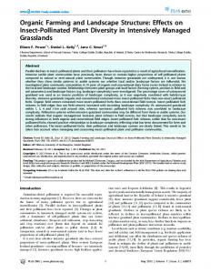
Fig. 1. Schematic illustration of the surface heat budget over (a) bare soil and (b) vegetated land. The roughness of the surfaces (and for the vegetation, its displacement height) will influence the magnitude of the heat flux. Dew and frost formation and removal will also influence the heat budget.

2. Physical linkage between the surface and atmosphere If we assume that vertical fluxes dominate, the energy and moisture balance between the ground and the overlying atmosphere is schematically illustrated in Figs. 1 and 2 for a non-precipitation atmosphere. As discussed in more depth in Pielke (1984), surface interfacial budget equations can be

written to describe the flux of heat and water into and out of the ground. There are several parameters in these budgets which are directly dependent on the soil type and on the vegetation characteristics. For soil, these parameters include density, porosity, texture, thermal diffusivity, hydraulic conductivity, and photometric properties. For vegetation, these parameters include leaf area index as a function of height,

136

BARE diffusivity of water

1

Transpiration

diksivity of water from soil Fig. 2. Schematic illustration of the surface moisture budget over (a) bare soil and (b) vegetated land. The roughness of the surface (and for the vegetation, its displacement height) will influence the magnitude of the moisture flux. Dew and frost formation and removal will also influence the moisture budget.

stomata1 resistance, albedo, aerodynamic roughness, displacement height, percentage coverage, and photometric properties. These parameters are discussed in some detail in Pielke (1984, Chapter 11) and elsewhere. Values for a number of these parameters are given in Table 1 through 7. Since the surface heat and moisture budgets are functions of the values of these parameters, landscape changes, in general, will alter the balance of the terms in Eqs. (1) and (2). An example of a surface heat budget analysis in the absence of vegetation is shown in Fig. 3 . Since these equations represent boundary conditions for the atmosphere, changes in atmospheric conditions will similarly be expected.

To illustrate the sensitivity of atmospheric conditions to even modest changes in surface characteristics, the earth’s global energy budget can be written as o~

= s(i - A ) ,

(@=

5.67 x 10-8wm-2~-4)

(1)

where we assume the earth radiates as a blackbody with a temperature TE. S is the solar constant ( S = 1380 WmP2)and A is the albedo. While not intending to represent the actual earth’s atmospheric response, this simple energy balance analysis is presented to illustrate the sensitivity of the earth’s climate to even very small changes in land use. Henderson-Sellers (1980) and Henderson-Sellers and Gornitz (1984) present two examples of preliminary

/

137 Table I . Albedos of shortwave radiation for assorted types of ground coversa (from Pielke 1984). Ground cover Fresh snow

A

0.75-0.95", 0.70-0.95', 0.80-0.95', 0.95e Fresh snow (low density) 0.85s Fresh snow (high density) 0.65f Fresh dry snow 0.80-0.959 Pure white snow 0.60-0.708 Polluted snow 0.40- 0.509 Snow several days old 0.40-0.70b, 0.70', 0.42-0.70', 0.40e Clean old snow 0.55s Dirty old snow 0.45f Clean glacier ice 0.35f Dirty glacier ice 0.25f Glacier 0.20-0.40e Dark soil 0.05-0. 15b, 0.05-0.159 Dry clay or gray soil 0.20-0.35b, 0.20-0.35g Dark organic soils 0.10f Clay 0.20s Moist gray soils 0.10-0.20g Dry clay soils 0.20-0.35d Dry light sand 0.25-0.45" Dry, light sandy soils 0.25-0.45s Dry, sandy soils 0.25-0.45' Light sandy soils 0.35f Dry sand dune 0.35-0.45", 0.37' Wet sand dune 0.20-0.30b, 0.24' Dry light sand, high sun 0.35s Dry light sand, low sun O.6Of Wet gray sand 0.10f Dry gray sand 0.20s Wet white sand 0.25s Dry white sand 0.35f Peat soils 0.05-0.15d Dry black coal spoil, high sun 0.05s Dry concrete 0.17-0.27b, 0.10-0.35e Road black top 0.05-0. l o b Asphalt 0.O5-0.2Oe Tar and gravel 0.08-0.18' Long grass (1.O m) 0.16e Short grass (2 cm) 0.26e Wet dead grass 0.20f Dry dead grass 0.30f Typical fields 0.20f Dry steppe 0.25', 0.20-0.309 Tundra and heather 0.15' Tundra 0.18-0.25', 0.15-0.20g Meadows 0.15-0.258 Cereal and tobacco crops 0.25f Cotton, potatoes and tomato crops 0.20s Sugar cane 0.15f Agricultural crops 0.18-0.25e, 0.20-0.30'

Table 1. Continued. ~____

Rye and wheat fields Potato plantations Cotton plantations Orchards Deciduous forests-bare of leaves Deciduous forests-leaved Deciduous forests Deciduous forests-bare with snow on the ground Mixed hardwoods in leaf Rain forest Eucalyptus Forest pine, fir, oak coniferous forests red pine forests Urban area

0.10-0.259 0.15-0.25g 0.20-0.259 0.15-0.20' 0.15e 0.20e 0.15-0.209 0.20' 0.18f 0.15s 0.20f 0.10-0.18' 0.10-0.15g, 0.10-0.15' 0.10f 0.10-0.27 with an average of 0.15e -0.0139 0.0467 tan 2 1 2 A 2 0.03h

+

Water aThe smaller number is for high solar zenith angles, while the larger albedo is more representative for low sun angles. bFrom Sellers (1965:21). CFromMunn (1966:15) 'From Rosenberg (1974:27).

eFrom Oke (1973:15,247). From Lee (1978:58-59). gFrom de Jong (1973).

hFrom Atwater and Ball (1981:879).

work on assessing actual climate impacts due to albedo changes, however, this important issue requires additional study. Differentiating (1) with respect to A yields aTE 4~- Ti 8A

=

- S,

which for small changes can be approximated by 4j3

AA

Ti

=

- S , or AT,

=

- SAA ~

T&

'

Using the values of S and u given above, AT,

=

-6.08 x 109 (

AA =.

~ 4 )

'E

Selecting a reasonable global-averaged earth temperature of T, = 283"K, (2) can be written as AT, = 268AA.

(3)

138 Table 2 . Representative values of aerodynamic roughness for a uniform distribution of assorted types of ground cover (from Pielke, 1984).

Aerodynamic roughness 20

Icea Smooth mud flatsg Snowa Sanda Smooth desertg Smooth snow on short grassC Snow surface, natural prairie Soilsa Short grassa Mown grassC

Long grassa Long grass (60-70 cm)

Agricultural cropsa

Height of ground cover

0.005 cm 0.1 cm 0.1-1 cm 0.3-1 cm 0.2 cm 0.7 cm 2.4 cm with Vat 2 m = 2ms-1 1.7 cm with P a t 2 m = 6.8 m s-] 4-10 cm 15 cmg, 9 cmc with P a t 2 m = 1.5 m s-l 11 cmg, 6.1 cmCwith Vat 2 m = 3.5 m s-1 8 cmg, 3.7 cmCwith P a t 2 m = 6.2 m srl 4-20 cme

Deciduous forestsa

50-1 me 1-6 me

Coniferous forestsa

1-6 me

4-m high buildings with lot areas of 2000 m2 and a 50 m2 silhouettea 20-m high buildings with lot areas of 8000 m2 and a 560 m2 silhouette 100-m high building with lot areas of 20.000 m2 and a 4000 m2 silhouette Rural Delmarva peninsula” Pakistan desertC

aFrom Oke (1978). bFrom Snow (1981). CFrom Priestly (1959). dUsing (7-31).

D

0.001 cm 0.001 cm 0.005-0.01 cm 0.03 cm 0.03 cm

2-10 cm 1.5 cm 3 cm 4.5 cm

25 cm to 1 m

-40 cm to 2

me Orchardsa

Displacement height

- 5 m to 10 me 10 m to 60 me 10 m to 60 me

-

5 cmd

4m

70 cmd

20 m

1000 cmd

100 m

33 cm (for north-west flow) 0.03 cm eUsing (7-46). fusing (7-45). gFrom Sellers (1965).

-27--1.3 mf -3.3--6.7 mf

- 6.7- - 40 mf -6.7--40 mf

139 Tuble3. Soil parameters as a function of eleven USDA (United States Department of Agriculture, 1951) textural classes and peata (from Pielke, 1984).

Soil type

%

Sand Loamy sand Sandy loam Silt loam Loam Sandy clay loam Silty clay loam Clay loam Sandy clay Silty clay Clay Peat

.395 ,410 .435 .485 .45 1 .420 .477 .476 .426 .492 ,482 .863

*S

- 12.1 - 9.0

-21.8 -78.6 -47.8 - 29.9 - 35.6 - 63.0 - 15.3 - 49.0 - 40.5 - 35.6

K,

b

"wilt

PiCi

.01760 .01563 .00341 .00072 .00070 .00063 .00017 .00025 .00022 .00010 .00013 .00080

4.05 4.38 4.90 5.30 5.39 7.12 7.75 8.52 10.40 10.40 11.40 7.75

.0677 .0750 .I142 .1794 .1547 .1749 .2181 .2498 .2193 .2832 .2864 .3947

1.47 1.41 1.34 1.27 1.21 1.18 1.32 1.23 1.18 1.15 1.09 0.84 -

aUnits for soil porosity (a)are centimeters per centimeters cubed, saturated moisture potential (qS)is in centimeters, and saturated hydraulic conductivity (K,J is expressed in centimeters per second. The exponent b is dimensionless. Permanent wilting moisture content (I,,,,~~) is in centimeters cubed per centimeters cubed, and it corresponds to 153 m (15 b) suction. Dry volumetric heat capacity @,c,) is in joules per centimeter cubed per degree Celsius. The first four variables for the USDA textures are reproduced from Clapp and Hornberger (1978). Table adapted from McCumber (1980). Table 4. Representative values of thermal conductivity v, specific heat capacity c, density r,and thermal diffusivity K,, for various types of surfaces (from Pielke, 1984).

k,

Surface

v(Wm-'K-I)

c(J kg-IK-1)

p(kg

Concrete Rock Ice

4.60a 2.93a 2.51a

879a 753a 2093a; 2100b

2.3a x 103 2.7a x 103 0.9a x 103: 0 . w x 103

2.3a x 1.4a x 1.3a x 1.16b x

2093a; 2090b

0.2a x 103: o.iob x 103

2093a; 2090b

0.8a

0.03a; 0.02C; 0.025b

1005

0.0012a x 103

0.3 x 10-6; O.lb x 10-6 1.0a x 10-6; 0.4b x 21a x 10-6

0.25b 0.63a 1.12a 1.33a 1.5gb

890b 1005a 1172a 1340a 1550b

i.6b i.7a i . i.9b 2.0b

x 103 x 103 x ~103 x 103 x 103

0.18b x 10-6 0.37a x 0.53a x 0.52b x 0.51b x

0.30b 1.05a 1.95a 2.16a 2.20b

800b 1088a 1256a 1423a 1480b

i.6b i.7a i.8a i.9a 2.0b

x 103 x 103 x 103 x 103 x 103

0.24b 0.57a 0.85a 0.80a 0.74b

0.06b 0.10a 0.29a 0.43a 0.50b 0.llC 0.63a; 0.57b

1920b 2302a 309ga 3433a 3650b 1256c 4186a

0.3b x 103 0.4a x 103 0.7a x 103 i . o a x 103 i.ia x 103 o . 3 ~x 103 i.oa x 103

Snow new old Nonturbulent air Clay soil (40% pore space) dry 10070 liquid water 20% liquid water 30% liquid water 40% liquid water Sand soil (40% pore space) dry 10% liquid water 20% liquid water 30% liquid water 40% liquid water Peat soil (80% pore space) dry 10% liquid water 40% liquid water 70% liquid water 80% liquid water Light soil withh roots Liquid water aFrom Lee (197897). bFrom Oke (1973:38). CFromRosenberg (1974:66).

m-3)

x 103; 0 . w x 103

= v/pc(mZs-l)

x x x x 10-6 x

0.10b x 10-6 0.12a x 10-6 0.13a x 0.13a x 0.12b x 10-6 O.3Oc x 0.15 x

140 Table 5. Emissivities of longwave radiation for representative types of ground covers (from Pielke, 1984). Ground cover

&

Fresh snow Old snow Dry sand Wet sand Dry peat Wet peat Soils Asphalt Concrete Tar and gravel Limestone gravel Light sandstone rock Desert Grass lawn Grass Deciduous forests Coniferous forests Range over an urban area Pure water Water, plus thin film of petroleum oil

0.99' 0.82a 0.95b, 0.914c 0.9gb, 0.936c 0.97b 0.9gb 0.90-0.98' 0.95', 0.956c 0.71-0.90', 0.966' 0.92a 0.92b 0.9gb 0.84-0.91' 0.97b 0.90-0.95' 0.97-0.9ga; 0.95b 0.97-0.9ga; 0.97b 0.85-0.95' 0.993' 0.972'

700-1

ground 6oo- heat 5oo -conduction 400-

'From Oke (1973:15, 247). bFrom Lee (1978:69). CFromPaltridge and Platt (1976:135).

For T, = 263"K, AT, = -334AA; for T, = 288"K, AT, = - 254AA; for T, = 303"K, AT, = - 218AA Since the ocean and other water bodies cover about 75% of the earth, and the albedo is not expected to change, we are concerned only about albedo changes on land as viewed from space. Thus let AA = 8AlanJ where f is the fraction of the earth that is land cf=O.25). Equation (3), therefore, becomes A%

7

-67AA.

(4)

Using (4), AT, = -6.7"C for a 10% increase in the albedo of land. Even for a 1% increase, AT, = - 0.67"C which is the same magnitude as the postulated greenhouse gas warming! In the next section, a more detailed evaluation of the impact of landscape changes on local and regional climate is presented.

300200 -

2 c

4

A

longwave irradiance from the ground

turbulent rensi ble heat flux

4

0-100-200.

-300

t

-400-

long wave irradiance from the atmosphere

- 500-

-600j

.)

(I- A)

-700

Solar lrradiance Fig. 3. Average heat fluxes at 1300 LST observed over the Empty Quarter of Saudi Arabia. A positive value represents a loss to the surface and a negative value is a gain. The sum of the fluxes equals zero. Over the Empty Quarter, the latent heat flux is essentially zero (from Eric Smith, CSU, 1982, personal communication and Pielke, 1984).

Observational and modeling evidence of the role of surface properties in influencing local and regional climate

Observational evidence On the microclimate scale, there have been numerous studies which document near surface climate conditions as a function of surface conditions (e.g., Rosenberg 1974; Oke 1978; and Lee 1978). Thus we should expect that when these surface conditions cover a large enough area, the local and regional climatic conditions will be affected. In addition, if two or more regions of different surface properties are juxtaposed, thermally-forced wind circulations and changes in atmospheric thermodynamic properties are often likely to result, since the atmosphere will be heated or cooled at different rates over the different land use areas. Dalu et al. (1990) present an analytical model which indicates the size of heated/cooled regions which must occur before a significant mesoscale circulation will result.

141 Table 6. Representative values of leaf area index LA transmissivity, absorption, and albedo for shortwave radiation ( y, respectively), and emissivity for longwave radiation (cf) for various types of vegetationa (from Pielke, 1984). -

a

LA maize, rice June 1 Mid July September 1 Mid Oct. Cotton Wheat, barley Prairie grasslands Green Dead Meadow

Coniferous forest Deciduous forest Aspen (in foliage)

0 1.8 4 6 2 4

A,

-

- 0.90

0.0 -0.30 0.65 -0.70 -0.57 -0.55

-0.55 -0.15 -0.10 0.23 -0.25

-

-

-1 -4 2 4 6 2 4

-0.20 0.08

-

-0.72 -0.82 0.70 -0.82

2 4 6

- 0.45 - 0.23 - 0.06

-0.35 0.65 -0.82

- 0.63 - 0.12

- 0.72

-0.30 -0.25

- 0.59

Ef

0.95 0.95 0.95 0.95 0.95 0.95

-0.10 -0.15 -0.20 0.20 0.20 0.20

-

0.96 0.96 0.96 0.96 0.96 0.97 0.97

- 0.48

Oak 30-year old stand No foliage Full foliage 160-year old stand No foliage Full foliage

-

-

- 0.10 -0.10

- 0.20 -0.12 -0.12

-0.25

0.12 0.16

-0.58

0.12 0.16

aEstimated from data given in papers published in Monteith (1975b). bThese values of E~ were obtained from Lee (1978:69).

Table 7. Characteristic values of surface biological resistance of a canopy to loss of watera (from Pielke, 1984). Type of vegetation Cotton field 0600 LST (noon) 1800 LST Sunflower field LA = 1.8 LA = 3.6 Coniferous forest 0600 LST Spruce Hemlock Pine Noon Spruce Hemlock

rc(s m-I)

- 130 - 17 - 330 110 80

- 20 - 240 - 50 - 100 - 150

Pine 1800 LST Spruce Hemlock Pine Prairie grasslands 0800 LST late July mid September 1200 LST late July mid September 1800 LST late July mid September

aValues estimated from published values given in papers presented in Monteith (1975b).

- 130 - 120 - 200 -310

- 100 - 150 - 100 - 500 - 150

- 550

a, and A )

142

36

K1(

Fig. 4. Composite of GOES derived surface temperature at 1300 LST for the period 1 August 1986 to 15 August 1986 for northeast Colorado (FC-Fort Collins; FM-Fort Morgan; GR-Greeley; W-Windsor; B-Briggsdale). Irrigated areas are shaded (from Segal el al. 1988).

Figures 5-8 present an example of an observational study of weather changes during a summer period between an irrigated area and a short grass prairie over northeast Colorado (see Fig. 4 for the

location where the observations were made). The irrigated area, characterized by large evapotranspiration, as contrasted with the prairie whose vegetation is under water stress, is substantially cooler at the surface even in the climatological average, as seen from a 15 day composite of infrared images collected from a geostationary satellite (GOES) every day at the same time during the summer of 1986 (Fig. 4). Surface temperature differences higher than 10°C are evident in this composite. The size of the irrigated area is illustrated by the stippling in Fig. 4. Aircraft measurements and radiosonde soundings across this region, reproduced from Segal et al. (1989), document the depth to which these differences exist. Figures 5 and 6 present analyses of potential temperature (defined as the temperature of the air if the pressure was increased to 1000 mb) and mixing ratio of water (defined as the ratio of the density of water vapor to the density of air). The

320.0

-

c

Y

m 316.0

320.e

-x

0

317.0

320.e

c:

x

a

317.0

320.0

a:

-Y

a

317.0

t . . . . . . . . . , . . . : e

20

38

DISTANCE (km)

re

50

Fig. 5. Measured potential temperature around noon on July 28, 1987 from Briggsdale to Windsor at the altitude of (a) = 140 m, (b) -240 m, (c) -345 m, and (d) ~ 4 4 m 0 above the ground as measured by aircraft. The observed crop-dry land boundary is indicated by an arrow with dry land on the left (from Segal el al. 1989).

143 12.5

-

a :

1

I

0

-.. s

0

--

7.5 13.0

I

A 0

-. b

0

8.0 12.0

-

c:

I

s 0

-. b

0

-

7.8

13.8

,

.

,

. . . .

,

.

. . .

,

. . . .

~

I

.

.

d l

I

0

a

-. b

0

8.9 8

18

28

39

50

DISTANCE (hm)

Fig. 6. The same as in Fig. 5 except for moisture mixing ratio (from Segal et al. 1989).

differences in atmospheric conditions diminishes higher up, although there is still evidence of the differences even at 440 m. Turbulence intensity is also much more substantial over the natural grassland (as a result of the greater surface heating), as evident in Fig. 7 where the measured horizontal velocities are plotted. Vertical soundings of temperature and dew point temperature over the irrigated area near Windsor and over the grassland area near Briggsdale further document the difference in atmospheric conditions between the two regions (Fig. 8). Pielke and Zeng (1989) suggest, based on this sounding, that severe thunderstorms are more likely over the irrigated area than over the prairie land since the added water vapor provides much greater buoyant energy for the cumulus cloud convection. Also, biometeorological heat load can be higher as a result of the higher relative humidities (e.g., see Segal et al. 1982). Figures 9-13, reproduced from Cramer (1988), provide a similar analysis except between snow cover and snow-free prairie areas in Colorado

during the winter. As evident in the figures, a welldefined cool pocket is evident over the snow. Also present is pollution in the very stably stratified air over the snow cover (Figs. 11 and 13c). For the observations presented here, the snow cover gradient was the result of the track of air extratropical cyclone. Such snow cover differences, however, are also noted due to differences in snow melt rates as a result of different land use (e.g., an urban area melts more quickly than the surrounding rural areas).

Modeling evidence Mathematical models provide the opportunity to quantitatively evaluate the specific impact of changes of surface forcing on climate. However, these models are only approximations of real world conditions and must, therefore, be validated against observations. The model results presented in this section use a modeling system which has been validated for a wide range of thermally-forced atmo-

144

-I

6.0

f E

>

-1

0.0 7.0

.

.

.

.

.

.

.

.

.

.

.

.

.

.

.

.

.

.

.

.

.

.

.

.

.

.

f E

>

--

0.0 7.0

I

-

f E

>

-1

0.0 7.0

-

f E

>

0.0

20

0

30 DISTANCE (km)

se

40

Fig. 7. The same as in Fig. 5 except for horizontal wind speed (the dashed line indicates an eye estimate of the running mean (from Segal et al. 1989).

0

T20

I

40

60

80

DISTANCE (km)

/

-10

0

.

,

/

10

20

/

30

I

40

T ("C) Fig. 8. Radiosonde measurements of potential temperatures (right side) and dew point temperatures (left side) for the dry area near Briggsdale (dashed lines) and the irrigated area near Windsor (solid lines) at 1213 MST of July 28, 1987 (from Pielke and Zeng 1989). The precipitable water in the layer from the surface to 740 mb is 1.1 g c r r 2 for the irrigated area sounding and 0.9 g cm-2 for the dry land area.

Fig. 9. Measurements of surface albedo and surface infrared temperature of a region of southeast Colorado on February 12,1988, as viewed from an aircraft flight at 95 m. The data were measured from 12:48:48--13:13:24MST. Thedarklineindicates snow-covered portion of transect where the right portion of the snow-covered area was patchy. The arrow at the base of the figures indicates location of the frozen Arkansas River (from Cramer 1988).

spheric systems, including land-sea breezes and mountain-valley circulations (e.g., see Pielke 1984, Appendix B). The details of the model and the parameteriza-

145 3001

m ,

u n c w

710 rn

!

i

Q 290 Q

GG Y

290

I80 m

-

Q

29

300

I

95 rn

4 , -2

290

,

40

60

80

0

DISTANCE (km) Fig. IO. Potential temperature at four flight levels for the same case study as in Fig. 9. The cross sections were made with time from 95 m to 710 m, with the later flight concluding at 14:08 MST (from Cramer 1988).

710 m

-100

I

180 m J

z

-

n

t

I

95 m

60

80

DISTANCE (km) Fig. I f . Same as Fig. 10 except for cloud condensation nuclei (from Cramer 1988).

. ,

- ,g

DISTANCE 40 (km)

60

80

Fig. 12. Same as Fig. 10 except for vertical velocity (from Cramer 1988).

tions for soil and vegetation physics is given in Segal et al. (1988), and Avissar and Pielke (1989), and results from those papers are presented here. Figure 14a, from Segal et al. (1988), presents results for an idealized simulation (SBS) of a seabreeze where the thermal forcing is caused by the heating of the bare, dry ground, as contrasted with the constant temperature ocean. Figure 14b presents results for an identical simulation except the ocean is replaced by unstressed vegetation (C2). This result suggests that areas of unstressed forest, grass, or cropland adjacent to dry, unvegetated land can result in local wind circulations as intense as a sea breeze. Pielke and Zeng (1989) use the results of Fig. 14b to propose that thunderstorm severity could be particularly strong in the horizontal wind convergence region that develops because of this differential surface heating. When the bare soil is moistened (not shown), the local wind circulation essentially disappears (alhough enhanced cumulus convective instability will remain because of the higher water vapor in the lower levels of the atmosphere). Similarly, when the fractional coverage of land by unstressed vegeta-

146

8Wl

8iKi

Fig. 13a. Vertical profile measurement of potential temperature for the case study given in Fig. 9. Measurements over snow-free prairie were made from 12:30:00-12:57:10 MST. Measurements over snow were made from 14:16:55-14:35:00 MST (from Cramer 1988).

p" I0 m-I

& 10*-7

Fig. 13b. Same as Fig. 13a except for density of water vapor (from Cramer 1988).

C (N cm.) I

C (NmJI

Fig. 13c. Same as Fig. 13a except for cloud condensation nuclei (from Cramer 1988).

tion is reduced compared with the simulation shown in Fig. 14d, the intensity of the thermallyforced wind circulation is reduced. The presence of vegetation also permits the atmosphere to tap water which is below the surface in the root zone. As shown in Fig. 14c, this water is unavailable over the bare soil even though the water amounts below 5 cm are the same below both the bare soil and the vegetation. If the vegetation were replaced with bare soil in Fig. 14c, with the same vertical distribution of water in the soil, no mesoscale circulation would develop. Using a more accurate representation of the influence of small-scale landscape inhomogeneities on the surface heat and moisture budgets, Avissar and Pielke (1989) describe the cumulative effect of these inhomogeneities on local and regional climate. For example, Fig. 15, reproduced from that paper shows the simulated sensible heat fluxes and surface temperatures during a typical midlatitude summer day for a dry soil region with 50% sloped to the north and 50% sloped to the south with slope angles of (a) 45", and (b) 15", adjacent to a homogenous dry flat region. The global value is the fractionally weighted value of the north- and southfacing slopes. The solar irradiance on a unit area of the surface as a function of time for differently oriented slopes is shown in Fig. 17. The different values, of course, are a direct response to the orientation of the sun with respect to the ground during the day. The influence of these gradients of sensible heat flux on the local and regional weather is illustrated in Fig. 16, where flow from the hilly region to the flat area is evident, particularly for the steep slope simulation. Figures 18 and 19 present the identical experiment except the north facing slopes are assumed to

Fig. 14. Vertical cross section of the simulated domain for the cases (a) SBS (land-sea contrast, where the dark segment indicates the sea); (b) C2 (unstressed vegetation with a uniformly moist soil - dry, bare soil contrast, where the dark segment indicates the vegetation; (c) C3 (unstressed vegetation - bare soil contrast with dry soils in both cases in the upper 5 cm of the soil, and moist below that level); and (d) C5 (same as C3 except only 25% of the ground is covered by vegetation) at 1400 LST for (i) u - west-east component of the wind in m s-l (dashed contours indicate negative component-easterly), (ii) w - vertical wind component in cm s-l (dashed contours indicate negative component-downward vertical velocity, (iii) 0- the potential temperature in K, (iv) q- the specific humidity in g kg-I, (v) the sensible (solid line) and latent (dashed line) heat fluxes at the surface (adapted from Segal et al. 1988). Aerodynamic roughness of z, = 4 cm and 10 cm were defined for bare soil and the vegetation (i.e., grass) used in these simulations, respectively.

147

I

i l

I

I

8 8 8 " 200"

]a n

0

W

148

2 500 X

LL

5 300 W -J

$100-

z

-1001

I

I

C8

10

I

I

12

14

I

16

-100 O

' 08

10

TIME (LST)

12

14

I6 L

TIME (LST)

a

W

a

z

F 35W

u a

/

-.-.

/

FLAT DOMAIN

a

---- SOUTKFACING NORTH-RLCING

2 25-

-Cu)BAL I

I

I

iL 3

m

L

I

25

08

10

12

14

16

TIME (LST)

(b) Fig. IS. The diurnal variation of sensible heat flux and surface temperature simulated for a horizontal dry surface and for dry northfacing and south-facing slopes. The inclinations of the slopes are (a) 45", and (b) 15" (from Avissar and Pielke 1989).

consist of unstressed vegetation, while the south facing slopes are dry and bare. Here, the low-level flow is towards the flat area when this area is dry, while the flow is towards the hilly region when the flat area is covered by unstressed vegetation. As seen in Fig. 19, the flow is towards the region with the larger turbulent sensible heat flux. Figure 20 photographically illustrates the type of terrain which is represented in Figs. 18 and 19. This distribution of vegetation is common in the western U.S. (e.g., see Whittaker and Niering 1965). Figures 15 and 16 suggest the alteration in the summer afternoon climate in this region if the northfacing slopes were deforested. The influence of urbanization on local and regional climate is demonstrated in Figs. 21 and 22 where the urban area is assumed to be 40% agricultural crops, 10% water bodies, 30% forests, and 20% built-up areas, and is adjacent to a surrounding area which consists of (a) bare, dry land, and (b) land completely covered by unstressed vegetation. When the surrounding terrain is bare, dry soil, the

flow at low levels is out from the developed area (Fig. 21a), whereas air moves toward the developed area if unstressed vegetation is on it periphery. These model results suggest that land use changes and changes in their spatial distribution can cause major alterations in local and regional climate. Additional observational studies are required to further document actual influences under real-world, non-idealized situations. Generalization to global climate and climate change

The integrated effect on global climate of the present distribution of surface properties around the world is not known. It is unlikely that current generation general circulation models can provide this information since they utilize very coarse horizontal resolution and have not attempted to include actual spatial variations in land use in their model simulations. Satellite imagery (e.g., Landsat) documents this small-scale irregularity in landscape caused as a result of man's activities. The difference

149

t "

lWOl 500

Fig. 16. Vertical cross section of the simulated region at 1400 LST for: (i) the horizontal wind component parallel to the domain (u) in m s-I, positive from left to right; (ii) the vertical wind component (w)in cm s-l, positive upward; and (iii) the potential temperature (0) in K, resulting from the contrast of a 60-km-wide hilly region (indicated by the dark underbar) which consists of 50% north-facing and 50% south-facing subgrid-scale dry slopes, and a 90-km wide dry flat region. The inclinations of the slopes are (a) 45", and (b) 15" (from Avissar and Pielke 1989).

0

U

8250-

*

*-*EAST

.-.-

----NORTH

......VEST

\

TIME (LST)

(b) Fig. 17. The diurnal variation of solar global radiation received at the surface of a horizontal surface and on slopes facing north, east, west, and south, on July 15 at a latitude of 37'N. The slopes inclinations are (a) 4 5 O , and (b) 15" (from Avissar and Pielke 1989).

150

2 500 X

3400

-

LA

t 300 W r. 200 -I

$1002 In

W

-lOOl

1

I

I

I

I

08

I0

12

14

16

0 -

-1mI

I

08

I

I

10

TIME (LSTI

I2

I

I

14

16

TIME (LST)

N.

700t

E

-

3600-

5 500

4-I 500-

LL

x 300

x 300

+

--

e

$200-

/M

5 100-

08

I

I

I

I

10

12

14

16

J

I

14

T I M E (LST)

-

- - - - - -

I-

I

16

T I M E (LST)

--Y 55W

W

a

a $45a

w

: p 35W U

Ba

2

-.-.

FLAT WMAIN SOUTH-FACING NORTH-FACING GLOBAL

25-

v)

I

1

08

---I

10

,

12

\

e

a

3 In I

I

14

16

25-

1

1

08

I

10

12

TIME (LST)

TIME (LST)

(a1

(b)

I

I

14

I6

Fig. 18. The simulated diurnal variation of sensible heat flux, latent heat flux, and surface temperature for a horizontal surface, a 45" north-facing slope completely covered by unstressed vegetation, and a bare, dry, 45" south-facing slope. The horizontal surface is (a) bare and dry, and (b) completely covered by unstressed vegetation (from Avissar and Pielke 1989).

Fig. 19. Vertical cross section of the simulated region at 1400 LST for: (i) the horizontal wind component parallel to the domain (u) in m s-l, positive from left to right; (ii) the vertical wind component (w)in cm s-l, positive upward; (iii) the potential temperature (0) in K; and (iv) the specific humidity (4)in g/kg, resulting from the contrast of a 60-km-wide hilly region (indicated by the dark underbar) which consists of 50% subgrid-scale, 45" north-facing slopes completely covered by unstressed vegetation and 50% bare, dry, 45" southfacing slopes, and a 90-km wide horizontal region. The horizontal region is (a) bare and dry, and (b) completely covered by unstressed vegetation (from Avissar and Pielke 1989).

151

30001

500

1

7

I

. , , , , , , , , ,., I

1

,, ,

) " ' " ' ' I

i

153

h

E

U

I-

I

(3

i

I

n

E Y

I-

I E I

a

-2000R 5'~"'-a

n

E

I-

-

I w 1000

~

30b

306

1

Fig. 22. Same as Fig. 19 except the dark underbar indicates a heterogeneous land surface which consists of 20% built-up areas and waste lands, 10% bodies of water, 40% agricultural crops, and 30% forests (from Avissar and Pielke 1989).

154 change in response to the atmospheric changes. Although on different time scales, a proper representation of the linkage cannot be achieved without including the details of the diurnal behavior of the surface moisture and heat fluxes. Acknowledgements

The study was supported by NSF grant # ATM8616662. This paper was invited as a plenary contribution to the March 15- 18,1989 LandscapeEcology Symposium in Fort Collins, Colorado. Ms. Dallas McDonald, as usual, competently completed the preparation and editing of the paper. The authors also appreciate the comments of Tim Kittel. References Anthes, R.A. 1984. Enhancement of convective precipitation by mesoscale variations in vegetative covering in semiarid regions. J. Climate Appl. Meteor. 23: 541-554. Avissar, R. and Mahrer, Y. 1988a. Mapping frost-sensitive areas with a three-dimensional local scale numerical model. Part 1: Physical and numerical aspects. J . Appl. Meteor. 27: 400413. Avissar, R. and Mahrer, Y. 1988b. Mapping frost-sensitive areas with a three-dimensional local scale numerical model. Part 11: Comparison with observations. J. Appl. Meteor. 27: 414-420. Avissar, R. and Pielke, R.A. 1989. A parameterization of heterogeneous land surfaces for atmospheric numerical models and its impact on regional meteorology. Mon. Wea. Rev. 117: 21 13-2136. Carson, D.J. and Sangster, A.B. 1981. The influence of landsurface albedo and soil moisture on general circulation model simulations. GARP/WCRP: Research Activities in Atmospheric and Oceanic Modeling. (Ed. I.D. Rutherford). Numerical Experimentation Programme, Report No. 2, 5.14-5.21. Charney, J.G., Quirk, W.J., Chow, S.H. and Kornfield, J. 1977. A comparative study of the effects of albedo change on drought in semi-arid regions. J . Atmos. Sci. 34: 1366-1385. Chervin, R.M. 1979. Response of the NCAR general circulation model to changed land surface albedo. Report of the JOC Study Conference on Climate Models: Performance, Intercomparison, and Sensitivity Studies, Washington,D.C. 3-7 April, 1978. GARP Publ. Series, No. 22, Vol. 1, pp. 563581. Cramer, Capt. James, 1988, M.S. Thesis: Observational Evaluation of Snow Cover on the Generation and Modification of Mesoscale Circulations. Colorado State University, 144 pp. Dalu, G.A., Pielke, R.A., Avissar, R., Kallos, G. and Guerrini,

A. 1990. Impact of terrain thermal inhomogeneities on mesoscale atmospheric flow: Theory of the subgrid-scale parameterization. J. Atmos. Sci, (submitted). Dickinson, R.E. and Henderson-Sellers, A. 1988. Modelling tropical deforestation: A study of GCM land-surface parameterizations. Quart, J. Roy. Meteor. SOC. 114: 439462. Garrett, A.J. 1982. A parameter study of interactions between convective clouds, the convective boundary-layer, and forested surface. Mon. Wea. Rev. 110: 1041-1059. Henderson-Sellers, A. 1980. Albedo changes - Surface surveillance from satellites. Climatic Change. 2: 275-281. Henderson-Sellers, A. and Gornitz, V. 1984. Possible climatic impacts of land cover transformations with particular emphasis on tropical deforestation. Climatic Change. 6: 231-257. Henderson-Sellers, A., Dickinson, R.E. and Wilson, M.F. 1988. Tropical deforestation: Important processes for climate models. Climatic Change. 13: 43-67. Kurbatkin, G.P., Manabe, S. and Hahn, D.G. 1979. The moisture content of the continents and the intensity of summer monsoon circulation. Met. Gid. 1-6. Lee, R. 1978. Forest micrometeorology Columbia University Press, New York. Lovelock, J.E. 1986. Geophysiology: A new look at earth science. Bull. Amer. Met. SOC.67: 392-397. Mahfouf, J.F., Richard, E. and Mascart, P. 1987. The influence of soil and vegetation on the development of mesoscale circulation. J. Climate Appl. Meteor. 26: 1483-1495. Manabe, S. 1975. A study of the interaction between the hydrological cycle and climate using a mathematical model of the atmosphere. Proc. Conf. on Weather and Food, Endicott House, Mass. Inst. Tech., Cambridge, Mass., 9-11 May 1975, 10 pp. McCumber, M.C. 1980. A numerical simulation of the influence of heat and moisture fluxes upon mesoscale circulations. Ph.D. dissertation, University of Virginia. 255 pp. Mintz, Y. 1984. The sensitivity of numerically simulated climates to land-surface conditions. The Global Climate, J. Houghton, Ed., Cambridge University Press, 79- 105. Miyakoda, K. and Strickler, R.F. 1981. Cumulative results of extended forecast experiment. Part 111: Precipitation. Mon. Wea. Rev. 109: 830-842. Oke, T.R. 1978. Boundary layer climates. Methuen, London. Pielke, R.A. 1984. Mesoscale meteorological modeling. Academic Press, New York, N.Y. 612 pp. Pielke, R.A. and Zeng, X. 1989. Influence on severe storm development of irrigated land. Nat. Wea. Dig. 14: 16-17. Rosenberg, N. 1974. Microclimate: The biological environment. Wiley, New York. Rowntree, P.R. and Bolton, J.A. 1978. Experiments with soil moisture anomalies over Europe. The GARP Programme on Numerical Experimentation: Research Activities in Atmospheric and Oceanic Modeling (Ed. R. Asselin). Report No. 18. WMO/ICSU, Geneva, August 1978, p. 63. Segal, M., McNider, R.T., Pielke, R.A. and McDougal, D.S. 1982. A numerical model simulation of the regional air pollu-

155 tion meteorology of the greater Chesapeake Bay area - summer day case study. Atmos. Environ. 16: 1381-1397. Segal, M., Avissar, R., McCumber, M.C. and Pielke, R.A. 1988. Evaluation of vegetation effects on the generation and modification of mesoscale circulations. J. Atmos. Sci. 45: 2268-2292. Segal, M., Schreiber, W., Kallos, G., Pielke, R.A., Garratt, J.R., Weaver, J., Rodi, A. and Wilson, J . 1989. The impact of crop areas in northeast Colorado on midsummer mesoscale thermal circulations. Mon. Wea. Rev. 117: 809-825. Shukla, J. and Mintz, Y. 1982. Influence of land-surface evapotranspiration on the Earth’s climate. Science. 215: 1498-1501. Sud, Y.C. and Smith, W.E. 1985a. The influence of surface roughness of deserts on July circulation - a numerical study. Bound.-Layer Meteor. 33: 1-35. Sud, Y.C. and Smith, W.E. 1985b. Influence of local land surface processes on the Indian Monsoon: A numerical study. J .

Climate Appl. Meteor. 24: 1015-1036. Sud, Y.C., Shukla, J. and Mintz, Y. 1988. Influence of land surface roughness on atmospheric circulation and precipitation. A sensitivity study with a general circulation model. J. Appl. Meteor. 27: 1036-1054. Walker, J. and Rowntree, P.R. 1977. The effect of soil moisture on circulation and rainfall in a tropical model. Quart. J . Roy. Meteor. SOC.103: 29-46. Watson, A.J. and Lovelock, J.E. 1983. Biological homeostasis of the global environment: The parable of daisyworld. Tellus. 35B: 284-289. Whittaker, R.H. and Niering, W.A. 1965. Vegetation of the Santa Catalina Mountains, Arizona: A gradient analysis of the south slope. Ecology. 46: 429-452. Yamada, T. 1982. A numerical model simulation of turbulent airflow in and above canopy. J. Meteor. SOC.Japan. 60: 439-454.