influence of local and adaptive mesh refinement on

VI International Conference on Computational Methods in Marine Engineering MARINE 2015 F. Salvatore, R. Broglia and R. Muscari (Eds)

INFLUENCE OF LOCAL AND ADAPTIVE MESH REFINEMENT ON THE TIP VORTEX CHARACTERISTICS OF A WING AND PROPELLER J. WINDT∗ AND J. BOSSCHERS Maritime Research Institute Netherlands (MARIN) P.O. Box 28 6700 AA Wageningen, The Netherlands web page: http://www.marin.nl ∗ : corresponding author: [email protected]

Key words: CFD, RANS, adaptive mesh refinement, propellers, tip-vortices Abstract. Two different methods to obtain nearly grid independent solutions for tip vortex flow were tested for a wing and a propeller. A priory mesh refinement inside a tube with a helix shaped centre line worked quite well, reducing the grid dependency of the minimum pressure in the vortex core significantly but the accuracy still depends on the initial mesh. Better results were obtained with adaptive mesh refinement using the jump based estimator. Projection of new created nodes to the exact geometry is required to obtain high accuracy.

1

INTRODUCTION

The prediction of tip vortex cavitation inception of propellers requires an accurate computation of the minimum pressure in the vortex core. However, obtaining high accuracy is challenging due to the large influence of both grid resolution and turbulence modelling [4],[7]. Insufficient grid resolution may give too large numerical diffusion which will spoil the accuracy of the calculation while improper turbulence modelling also leads to too high diffusion of the flow in the vortex core. This paper shows an investigation on how to obtain meshes with enough resolution to get nearly grid independent solutions for tip vortex flow while accepting the deficiencies of the applied turbulence model. Use is made of MARIN’s Navier-Stokes code ReFRESCO with the adaptive mesh refinement strategies as presented in [15] and [14]. The mesh adaptivity routines were recently improved by assuring a proper (dynamic) load balancing when running the code in parallel by redistributing cells among the processors. The main goals of the present research were to thoroughly test the adaptive mesh refinement routines and to evaluate two mesh refinement methodologies being a priory 1

J. Windt and J. Bosschers

mesh refinement and fully automatic adaptive meshing. The methods are applied to obtain grid independent solutions for tip vortex flow for two test cases: the flow around a rectangular half wing and the flow around a propeller in open water conditions. The mesh refinement methodologies are presented first, followed by a brief description of the two test-cases. The results for these test cases will then be presented in detail and the conclusions will be given at the end. 2

3

NOMENCLATURE Cpn : Propeller pressure coefficient [-] Cpn = Cp

:

Pressure coefficient [-]

Cp =

KQ

:

Propeller torque coefficient [-]

KQ =

P −P∞ 1 ρ(nD)2 2 P −P∞ 1 2 ρU∞ 2 Q ρn2 D5

MESH REFINEMENT FOR TIP VORTICES

The required grid density to capture tip vortices accurately is high and therefore adaptive meshing is required. Ideally the flow solver should determine the mesh resolution dynamically using some kind of criterion and adapt the mesh in an iterative procedure. A feature based criterion like the non-dimensional Q-criterion [9],[10] (see Figure 2) could be used or some kind of error estimator [1],[6]. On the other hand, for standard cases it might be worthwhile to define the refinement a priori, that is before the calculation is started, or apply it after an initial quick calculation on a coarse mesh. 3.1

A priory mesh refinement

To define the tip vortex region, use is made of an empirically defined tip vortex trajectory as implemented in MARIN’s boundary element method for propellers, PROCAL. The tip vortex region is described by a helix with a certain radius and pitch. This helix describes the centre line of a cylindrical volume with a given diameter. The helix radius is not constant but reduces downstream, modelling the contraction of the tip vortex. The contraction depends on the slip ratio of the propeller and on the distance from the blade. 3.2

Refinement criteria

To detect tip vortices several refinement criteria can be used. We considered to use two different kind of criteria, a feature-based criterion like the non-dimensional Q-criterion and an error estimator. The Q-parameter is the relative vortical strength given by the difference between the vorticity magnitude and the local strain rate. The non-dimensional Qcriterion is proposed by Kamkar [9] [10] with the idea that due the non-dimensionalisation the threshold parameter does not depend on the type of flow and the levels of vorticity. Obviously this aspect is required for a fully automatic mesh-refinement method. The Q-criterion is not (yet) applied for the propeller test-case because it has the disadvantage that it only refines the region in which the vortex is present and strong enough. This means that no refinement will be done in the region upstream the vortex and also in the 2


far wake where the vortex is too weak due to numerical diffusion. A second criterion, also introduced in the Streamline project [6], is an estimator based on jump values. This error estimator, following Bernard[1], is defined as: s e2e , (1) Je = 2kΦk2L2 with ee the local error of an element and kΦkL2 the L2 norm of a scalar variable. The local error of an element is approximated by e2e

N ∆ X (ΦL − ΦR )2 , = 4N k=1

(2)

with N the number of element faces and ∆ the volume of the element. The left and right values of a face, ΦL and ΦR , are simply given by the face neighbouring cell values. A difference with the Q-criterion is that now the complete flow domain will be refined, if necessary. 4

DESCRIPTION OF TEST CASES

To test the mesh refinement methods, we have chosen two different test cases being the flow around a wing and the flow around a propeller. 4.1

Rectangular half-wing

The first test case is a rectangular half-wing with NACA 0012 wing section and a rounded tip for which extensive wind tunnel measurements were performed by Chow et al. [3]. The experiments, performed for an incidence angle of 10◦ and Reynolds number based on chord of 4.35 × 106 , include seven-hole pressure probe measurements of the velocity field in the near field of the wing tip. This configuration has been used in the EU Streamline project [8] and ReFRESCO results have been analysed in detail in [11]. Other computational results are presented in e.g. [4] and [12]. The wing chord length is constant and equal to 4f t. The wing tip is rounded using a circular surface with diameter equal to the foil local thickness. The span, excluding the circular tip rounding is 3 ft. The size of the computational domain is defined by the size of the tunnel test-section with the inlet and outlet located 1.5 and 3 chord length upstream and downstream the wing respectively. The inlet velocity is equal to 170f t/s. At the outlet zero pressure is imposed. The angle of attack is 10◦ around the origin at c/4. The trailing edge is located at x/c = 0.75cos(10), i.e. at x/c approximately 0.74. The flow around the wing and tunnel wall connected to the wing is solved down to the wall, i.e. without wall functions. At the top, bottom and opposite side wall of the tunnel, wall functions have been used. Maximum y + values on the wing surface are below 0.05 for the coarsest grid (875k) and below 0.015 for the finest grid (27.9M). All calculations have been performed using the k − ω SST turbulence model. Convective fluxes are discretised using the QUICK scheme. 3


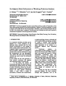
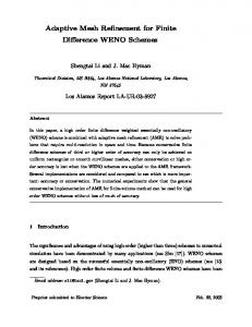
Figure 1: Left figure: overview of the pressure in the vortex core of the wing. Coarsest mesh. For one plane the mesh is plotted as well. Right figure: mesh distribution on the blade of the propeller (coarsest mesh). Thick lines indicate block boundaries.

4.1.1

Grid generation

The flow domain is discretised by a structured multiblock grid, built with GridPro, and contains 7754 blocks. The main reason for choosing block structured meshing instead of unstructured meshing is that it is much more easy to perform a systematic grid study. A systematically refined geometrically similar series of grids can be generated quite easily. With this series of grids an estimation of the computational error can be obtained. In [15] a simple straightforward block structure was applied, i.e. no special topology was chosen to increase the grid density around and in the vortex core. The calculations showed that a grid independent solution was not obtained although the finest mesh consisted of more than 11 million grid nodes. To overcome this problem a more advanced blocking is used. A tube shaped surface defines a high density region in and just around the tip vortex. This surface is dealt with as an internal surface and fixes the grid resolution inside the region. In total six grids were made with decreasing density, starting at 27.9 million cells down to 875.264 cells. The finest mesh has approximately 3 times more nodes in all three directions. An impression of the grid density and vortex is given in Figure 1. The figure shows the coarsest mesh solution. 4.2

Propeller

The second test case is a skewed tip-unloaded five-bladed propeller that is similar to the P5168 propeller for which the flow field was measured with 3-D LDV by Chesnakas and Jessup [2] while tip vortex cavitation inception was determined as well. This propeller was manufactured at MARIN as propeller No. S6468 of which the cavitation inception characteristics have been compared to those of P5168 in [13]. All tests were performed for open water conditions. The design advance coefficient, J, of the propeller equals 1.27. The 4


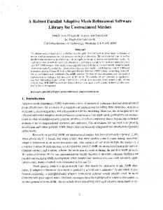
Figure 2: Local (a-priory) mesh refinement for the wing (left) and propeller (right). Refinement regions are marked by transparant surfaces. Cells marked by the Q-criterion show the vortex location.

present computations have been performed at J = Va /nD = 1.1 with an advance velocity Va = -15.258 m/s, rotation rate n of 43.27 rev/sec and propeller diameter D = 0.32 m. This diameter corresponds to the diameter of propeller S6468 while the propeller rotation rate was selected to match the Reynolds number of the tests with propeller P5168. The computational domain is cylindrical. At the farfield boundary, located at 2.5D distance from the propeller, pressure is imposed. At the inlet the advance velocity Va is imposed and at the outflow derivatives are set to zero. Both boundaries are located at 5D distance from the propeller. At the hub, free-slip is imposed and at the blades no-slip, without the use of wall function, is used. For all calculations the maximum y + is below one. All calculations were performed using the k − ω SST turbulence model. This test-case has also been used in other CFD studies, see e.g. [7]. 4.2.1

Grid generation

For the propeller a multi-block structured mesh was built with GridPro. Finding an appropriate block-topology for a modern propeller was not trivial, but the mesh can now be generated easily and automatically. The grid topology is built up by a series of 2D topologies, except at the blade tip where the mesh needs to be closed around the tip. To control the grid node distribution around the blade edge a tube (internal grid surface) is used with its centre line at the blade edge. No special topology was used to concentrate cells in the tip vortex region in the wake. Figure 1 shows the topology on the blade and shaft. The total number of blocks, for the five bladed propeller, is equal to 7450. A series of nine grids was generated. The finest mesh has approximately 3 times more nodes in all three directions and consist of 109 million nodes. The coarsest mesh consists of 4 million nodes. This is for the complete propeller, i.e. for all five blades. The a-priory mesh refinement is now done using three different tubes as illustrated in Figure 2 and is applied to one blade only. We focus on the tip vortex very close to the blade because this is the region where the minimum pressures are located as relevant for cavitation inception. Besides that, further downstream the solution will be inaccurate anyhow due

5


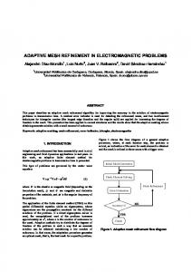
Figure 3: Overview of grids for the wing (left), convergence with grid refinement of the drag (middle) and minimum pressure in the tip vortex at x/c = 0.7 (right).

to limitations of the applied turbulence model. 5

RESULTS

The a priory mesh refinement was applied for the flow around the wing and for the flow around the propeller. The jump based estimator has also been applied to both cases but was only successful yet for the wing. The accuracy of the results will be verified, as much as possible, by the finest mesh solution for which an uncertainty estimation will be given. The calculation for the wing are presented first. 5.1

Wing

For the wing multiple series of calculations have been investigated. First a systematic mesh refinement study using six grids was performed followed by detailed studies on various aspects of local mesh refinement. Investigated were the influence of the size of the refinement region, the levels of refinement, and the initial grids. For most of these cases no projection of new created nodes to the exact geometry was made but for some cases the influence of such a projection was investigated. The notation to distinguish between the cases is straightforward. For example case G6STL 2 r0.10 means a-priory mesh refinement starting from grid G6 with projection to the STL geometry, using two successive refinement steps inside a tube with radius 0.10m. To get an estimation of the numerical uncertainty, the method proposed by E¸ca and Hoekstra [5] is used. Two examples of the uncertainty estimation are given in Figure 3. The figures show the best fit, in least square sense, that is used to calculate the uncertainty. The data of almost all calculations is in the asymptotic range, i.e. showing monotonic convergence. Even the coarsest mesh has already a high resolution in the vortex core, so all six grids could be used to estimate the uncertainty. The calculations show that for grid G1 the numerical uncertainty of the lift and drag is below 1%. In fact the coarsest mesh solution is already quite accurate with respect to these parameters. The numerical uncertainty of the vortex core pressure is significantly higher, especially at x/c = 0.9, i.e. 6


Figure 4: Minimum pressure in the vortex core versus the stream wise position for the wing. Left figure: grid G1 to G6. Dashed lines: G6,G4,G2, solid lines: G5,G3,G1. Squares mark the measurements. Right figure: results using local and adaptive mesh refinement. Not all results are plotted.

further downstream of the wing. For x/c = 0.6 to x/c = 0.8 the uncertainty is at or below 7%. Figure 4 plots the minimum pressure in the centre of the core as a function of the stream wise position x/c. The differences between the two finest grids are small. The measurements of [3] are indicated by square symbols. Ref. [4] showed that the number of elements along the vortex core radius must be at least 10 to accurately describe the vortex characteristics. This number was confirmed by the present grid refinement study [11]. A comparison with the measurements showed that the minimum pressure and (maximum) velocity in the core is in good agreement with the measurements, except behind the trailing edge. There the feeding of the vortex by the flow around the wing tip stops, the vortex gradually rolls-up and slowly decays. However, in the RANS calculations the decay is much too high due to a too large turbulent eddy viscosity in the core [4], [12]. The analysis in [11] also showed that the vortex strength is rather insensitive to the grid density and that behind the trailing edge the calculations slightly over predict the strength. For the local grid refinement a series of calculations was made to investigate the influence of the refinement region, the influence of the initial mesh and the influence of the accuracy of the geometry. For the wing case, the viscous core diameter is approximately 0.075m at x/c = 0.9. The a-priory mesh refinement is thus defined using a tube with radius 0.05m or 0.10m with a helix shaped centre line (in this case a straight line because a very high pitch is chosen). The refinement is only applied between x/c = 0.25 and x/c = 1.75. To test the sensitivity to the initial mesh, three grids have been used, G6, G5 and G4. For each grid (and using two tube radii for G6) one and two refinement step(s) were done. Another aspect investigated, which might influence the solution, is the adjustment of newly created nodes to the exact geometry by projection to the STL description of the wing. For the true adaptive mesh refinement study, the jump based estimator was selected. We used the combination of pressure and magnitude of velocity 7


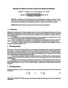
Figure 5: Propeller case: convergence with grid refinement of torque coefficient 10KQ and minimum pressure in the tip vortex. Middle figure: x = -0.007 m, right figure: x = -0.008 m.

with a threshold parameter Je < 10−5 . Figure 3 presents the drag versus the relative grid density. The figure shows the calculated drag coefficient using the series of grids G6 to G1, the fit through the results and the error estimate for the finest mesh G1. The adaptive/local mesh refinement results are indicated using different symbols. The calculations show that: • Obviously, mesh refinement in the cylindrical region does not improve the accuracy of drag and lift. The accuracy is determined by the grid density of the initial mesh. • Projection to the exact (STL) geometry slightly decreases the drag and lift. Whether or not this is an improvement depends on the case. • The best results are obtained with the jump based estimator, including the projection to the exact geometry (G6STL jmp 10−5 ). With respect to the minimum pressure in the core, plotted in Figure 4, the calculations show that with a priory mesh refinement: • Refinement in the cylindrical region reduces the pressure significantly. Differences between 1 and 2 refinement steps are small. • Increasing the diameter of the cylinder does not influence the accuracy. • The accuracy of the calculated pressure depends on the initial mesh. • Projection to the exact geometry does not improve the accuracy significantly. • Starting with mesh G4 gives comparable results as the reference solution (G1). Applying the jump based estimator as a refinement criterion, including the projection, works the best. Starting with the coarse mesh (G6) gives an accuracy comparable to the reference solution (G1) using 3 times less elements. Approximately 7.6M cells are added by the refinement. Without projection the accuracy is between G5 and G4. 5.2

Propeller

For the propeller a similar study was done. The uncertainty (presented in Figure 5) is estimated using a series of geometrically similar grids and the effect of a priory grid refinement is studied. Figure 6 gives an overview of all grids used and presents the 8


Figure 6: Propeller case: minimum pressure in the vortex core versus the x-coordinate. Grid study (left), a priory mesh refinement (right).

streamwise variation of the minimum pressure in the vortex core. Pressure contour plots showing the development of the vortex are given in Figure 7. The notation for the grid is similar as for the wing, for example G3STL 3 refers to grid G3 with 3 local refinement steps and projection to the exact (STL) geometry. The numerical uncertainties for the finest mesh solution were again obtained by a fit in the least squares sense. For the propeller however the results are not as consistent as for the wing because too few data points are in the asymptotic range. Figure 5 plots three examples of these fits, showing the convergence with grid refinement for the torque and the minimum pressure in the vortex core at two locations. For the torque (and similarly for the thrust) everything works fine and a reliable error estimation is obtained using all grids. For the pressure the fit is applied using the five (finest) grids only. At x = -0.007 m this gives an estimated uncertainty of the finest mesh solution of 13.2% with monotonic convergence. Taking four or six grids gives monotonic convergence too and the estimated error becomes 17.2% and 26.2% respectively. So the numerical uncertainty of the pressure coefficient is at least 13.2% and most likely less than 26.2%. Going just a bit further downstream at x = -0.008 m (right figure) shows a totally different uncertainty estimation. Using four grids gives an uncertainty of 42%, five grids gives 151% and six grids 101%. This analysis shows that in fact the mesh is still not dense enough and that for a more reliable uncertainty estimation a better multi-block structured topology should be used. So unfortunately the systematic grid study cannot be used to verify the local mesh refinement results. Nevertheless it shows the trend towards the grid independent solution. Remark that in comparison to the wing the computational domain is larger and five tips are present instead of one. Figure 4 shows that for the wing the minimum pressure at the vortex detachment region is not sensitive to the number of cells while Figure 6 shows that for the propeller the pressure in this region is influenced significantly by the gridding. The pressure at the vortex detachment 9


point is much smaller than the experimental cavitation inception pressure (equivalent to Cpn = −2.0). This aspect still needs to be further investigated. Next we focus on the local mesh refinement results presented in Figure 6 on the right. The overall minimum pressure distribution is significantly influenced by the gridding with values that are smaller than for the finest grid G9. The local mesh refinement results show that even with 3 refinement steps starting from grid G3, adding 8.4M cells to the refinement region for one blade, the solution is still not grid independent. The extreme grid dependency is not fully understood and may have several causes. Firstly, the grid density in the main stream direction is much lower than the density perpendicular to it. However this might be no problem because a systematic grid study, done in the past, of the decay of a vortex in a free stream showed that the solution is not very sensitive to the resolution in main stream direction. Nevertheless this should be investigated for the propeller case, because the tip vortex flow is different. Secondly the mesh is not aligned with the flow, which leads to more numerical diffusion compared to a flow aligned mesh. Also, the vortex for the propeller is weaker than for the wing and the viscous core is smaller. 6

CONCLUSIONS

A thorough mesh sensitivity study including uncertainty estimation was applied to investigate the minimum pressure in the tip vortex core of a rectangular half-wing. The calculations show that both a-priory local mesh refinement and adaptive mesh refinement improve the accuracy of the calculation significantly. However, with the applied a-priory grid refinement the results depended on the density of the initial mesh. With adaptive mesh refinement, using the jump based estimator, including the projection, the accuracy is comparable to the finest mesh solution, using 3 times less mesh elements. The uncertainty estimation for the propeller in open water conditions show that large grids are required to be in the asymptotic range for the minimum pressure. Although excessive local refinement was applied, no grid independent solution was obtained. This may be due to the fact that no special topology was used to locally refine in the tip vortex region and the much weaker tip vortex than for the wing. Whether the application of the jump based estimator to the propeller gives as good results as for the wing still needs to be investigated. References [1] Psaul-Emile Bernard. Discontinuous Galerking methods for geophysical flow modelling. PhD thesis, Universit´e catholique de Louvain, 2008. [2] C. Chesnakas and S. Jessup. Experimental characterization of propeller tip flow. In 22th Symposium on Naval Hydrodynamics, Washington DC, USA, 1998. [3] J. Chow, G. Zillac, and P. Bradshaw. Mean and Turbulence Measurements in the Near Field of a Wingtip Vortex. AIAA Journal, 35(10), Oktober 1997. [4] J. Dacles-Mariani, D. Kwak, and G. Zilliac. On Numerical Errors and Turbulence 10


[5]

[6]

[7]

[8] [9]

[10]

[11] [12]

[13]

[14]

[15]

Modeling in Tip Vortex Flow Prediction. International Journal for Numerical Methods in Fluids, 60:65–82, 1999. L. E¸ca and M. Hoekstra. A procedure for the estimation of the numerical uncertainty of CFD calculations based on grid refinement studies. Journal of Computational Physics, (262):104–130, 2014. C. Eskilsson and R. E. Bensow. A Mesh Adaptive Compressible Euler Model for the Simulation of Cavitating Flow. In MARINE 2011, IV International Conference on Computational Methods in Marine Engeneering, September 2011. C.T. Hsiao and G.L. Chahine. Scaling of Tip Vortex Cavitation Inception for a Marine Open Propeller. In 27th Symposium on Naval Hydrodynamics, Seoul, Korea, Oktober 2008. http://www.streamline-project.eu/. Streamline website, June 2011. S. J. Kamkar, A. Jameson, and A. M. Wissink. Automated Grid Refinement Using Feature Detection. In 47th AIAA Aerospace Sciences Meeting Including the New Horizons Forum and Aerospace Exposition, Januari 2009. S. J. Kamkar, A. Jameson, A. M. Wissink, and V. Sankaran. Feature-Driven Cartesian Adaptive Mesh Refinement in the Helios Code. In 47th AIAA Aerospace Sciences Meeting Including the New Horizons Forum and Aerospace Exposition, Januari 2009. N. Kamphuis. Analysis of ReFRESCO Computations Applied to a Tip Vortex of a Wing. MARIN Report 70017-3-RD, 2012. S.E. Kim and S.H. Rhee. Toward High-Fidelity Prediction of Tip-Vortex around Lifting Surfaces - What Does It Take. In International Symposium on Naval Hydrodynamics, 2004. T.J.C. van Terwisga, E. van Wijngaarden, J. Bosschers, and G. Kuiper. Cavitation Research on Ship Propellers - a Review of Achievements and Challenges. In 6th International Symposium on Cavitation, CAV2006, Wageningen, The Netherlands, 2006. J. Windt. Adaptive Mesh Refinement in Viscous Flow Solvers: Refinement in the Near-wall Region, Implementation and Verification. In 13th Numerical Towing Tank Symposium (NuTTS), September 2013. J. Windt and C.M. Klaij. Adaptive Mesh Refinement in MARIN’s Viscous Flow Solver ReFRESCO: Implementation and Application to Steady Flow. In MARINE 2011, IV International Conference on Computational Methods in Marine Engeneering, September 2011.

11


Figure 7: Propeller case: contour plots of the pressure coefficent at planes perpendicular to the vortex at x = -0.007 m, x = -0.008 m, ..., x = -0.012 m. From top to bottom: G1, G9, G3STL 3

12