Information-Cloning of Scale-free Networks Mahendra Piraveenan1,2 , Mikhail Prokopenko1 and Albert Y. Zomaya2 1
2
CSIRO Information and Communications Technology Centre Locked Bag 17, North Ryde, NSW 1670, Australia, School of Information Technologies, The University of Sydney, NSW 2006, Australia Corresponding author:
[email protected] Abstract. In this paper1 , we introduce a method, Assortative Preferential Attachment, to grow a scale-free network with a given assortativeness value. Utilizing this method, we investigate information-cloning — recovery of scale-free networks in terms of their information transfer — and identify a number of recovery features: a full-recovery threshold, a phase transition for both assortative and disassortative networks, and a bell-shaped complexity curve for non-assortative networks. These features are interpreted with respect to two opposing tendencies dominating network recovery: an increasing amount of choice in adding assortative/disassortative connections, and an increasing divergence between the joint remaining-degree distributions of existing and required networks.
1 Introduction Many biological networks, e.g. gene-regulatory networks, metabolic networks, and protein interaction networks are often characterized as complex scale-free networks. In this paper, we consider a task of information-cloning of a scale-free network, given its fragment and some topological properties of the original network. The “cloning” is interpreted information-theoretically: the resulting network may disagree with the original one in terms of specific node to node connections, but is required to have equivalent information transfer. The information-cloning task is partly motivated by needs of network manufacturing, where an “assembly-line” starts with a fragment and continues with “manufacturing” the rest, subject to topological constraints. Another motivation is regeneration of scale-free networks which are prone to percolation/diffusion of adverse conditions, as well as removal of highly connected nodes. Both demands (topologyoriented manufacturing and regeneration) are referred in this paper as network recovery. Recovery of networks can be attempted and evaluated in various ways. In this paper, we aim at a general measure in terms of mutual information contained in the network, or its information transfer. More precisely, we propose to judge success of the recovery with respect to the amount of information transfer regained by a resulting network. Various network growth models have been analyzed in literature [1–4]. One prominent model is the preferential attachment model, which explains power law degree distributions observed in scale-free networks [4]. In this model, the probability of a new node making a link to an existing node in the network is proportional to the degree of the target node. Newman [2] pointed out that this model does not take into account the degree of the source node in influencing the attachment probability, and suggested to consider another tendency for preferential association, measured via assortativeness. The 1
The Authors list is in alphabetical order.
networks where highly connected nodes are more likely to make links with other highly connected links are said to mix assortatively, while the networks where the highly connected nodes are more likely to make links with more isolated, less connected, nodes are said to to mix disassortatively. In both cases, the likelihood of creating a link depends on the degrees of both nodes. Both assortative and disassortative mixing is contrasted with non-assortative mixing, where no preferential connection can be established. The extent of assortativeness affects network’s resilience under node removal or percolation/diffusion of adverse conditions [2]. Our objective is an investigation of how successful is a network recovery in terms of assortativeness and information transfer. We note that this objective is different from investigation of networks’ robustness properties such as error tolerance, attack survivability, or network fragmentation that have been extensively studied [5–7]. For example, Moreno et al. [7] explored robustness of large scale-free networks faced with node-breaking avalanches (cascading failures when a failure of a node triggers subsequent failures of neighbours), and investigated how the random removal of nodes in a fixed proportion affects the global connectivity and functionality of scale-free networks. Stauffer and Sahimi studied scale-free networks with annealed disorder [8], when the links between various nodes may temporarily be lost and reestablished again later on, and observed a number of critical phenomena, e.g. “the existence of a phase diagram that separates the region in which diffusion is possible from one in which diffusion is impossible”. This study did not investigate, however, the role of assortativeness and information transfer in the diffusion process. Naturally occurring networks display various extents of assortative mixing, and it is often possible to measure or calculate the level of assortativeness in these networks [1]. However, it is not straightforward to (re-)grow a network with a level of assortative mixing specified a priori. We address this problem and propose a method to grow or recover a scale-free network with a given assortativeness. We also show that a network with perfect assortativeness can be grown for any desired degree distribution, whereas a network with perfect disassortativeness can be grown only if the corresponding ‘remaining degree distribution’ for the desired degree distribution is symmetric. Utilizing this method, we investigate recovery of scale-free networks in terms of their information transfer. Following Sol´e and Valverde [1], we define the information transfer as mutual information contained in the network, or the amount of general correlation between nodes. Importantly, the maximum attainable information transfer defines the network’s capacity, in analogy with information-theoretic notion of channel capacity — the maximum mutual information for the channel over all possible distributions of a transmitted signal. In general, information transfer is a vital indicator of complex non-linear behavior in self-organizing systems, and can be associated with predictive information, richness of structure (i.e. excess entropy), and physical complexity [9].
2 Assortativeness and Information Transfer We study assortativeness in scale-free networks described by power law degree distributions, formally specified as P (k) = Ak −γ u(k/Np ) where u is a step function specifying a cut off at k = Np . The degree of a node is the number of other nodes to which it is connected to. Let us consider a network with N nodes (vertices) and M links (edges), and say that the
probability of a randomly chosen node having degree k is pk , where 1 ≤ k ≤ Np . The distribution of such probabilities is called the degree distribution of the network. However, if a node is reached by following a randomly chosen link, then the remaining number of links (the remaining degree) of this node is not distributed according to pk . Instead it is biased in favour of nodes of high degree, since more links end at a highdegree node than at a low-degree one [2]. The distribution of such remaining degrees is called the remaining degree distribution, and is related to pk as follows: qk =
(k + 1)pk+1 , 0 ≤ k ≤ Np − 1 P Np j jpj
(1)
where pk is the degree distribution of the network, and qk is the remaining degree distribution of the network [2]. For scale-free networks, Eq. (1) yields that if γ = 1 (that is, p(k) = A/k before the cut off), the resulting remaining degree distribution is uniform, therefore symmetric. Following Callaway et al. [3] and Newman [2], we define the quantity ej,k to be the joint probability distribution of the remaining degrees of the two nodes at either end of a randomly chosen link. As pointed out by Newman [2], this quantity is symmetric in an undirected graph, that is ej,k = ek,j , and it obeys the sum rules P its indices forP ej,k = 1 and ej,k = qk . Assortativeness is formally defined [4] as a correlation jk
j
function which is zero for non-assortative mixing and positive or negative for assortative or disassortative mixing respectively: r=
1 X jk(ej,k − qj qk ) σq2
(2)
jk
where σq2 is the variance of the probability distribution qk . Here r lies between −1 and 1, whereby r = 1 means perfect assortativeness, r = −1 means perfect disassortativeness, and r = 0 means no assortativeness (random linking). If a network has perfect assortativeness (r = 1), then all nodes connect only with nodes with the same degree. For example, the joint distribution ej,k = qk δj,k where δj,k is the Kronecker delta function, produces a perfectly assortative network. If the network has no assortativeness (r = 0), then any node can randomly connect to any other node. A sufficiency condition for a non-assortative network is ej,k = qj qk . Perfect assortativeness and perfect disassortativeness are not exact opposites. Newman noted that if a network is perfectly disassortative then every link connects two nodes of different degrees (types) [10]. However, this requirement is not sufficient to generate an ej,k resulting in r = −1. In fact, the r = −1 case is possible only for symmetric degree distributions where qk = q(Np −1−k) : ej,k = qk δj,(Np −1−k) . In other words, for a network with remaining degrees 0, . . ., Np −1, a node with a degree k must be linked to a node with a degree Np − 1 − k. Nodes with identical degrees may still be connected in a perfectly disassortative network (e.g., when their degree j is precisely in the middle of the distribution q, i.e., Np is odd and j = (Np − 1)/2). Perfect disassortativeness is not possible for non-symmetric degree Pdistributions q, because the ej,k distribution must obey the rules ej,k = ek,j , as well as ej,k = qk . On the contrary, any j
degree distribution may give rise to a perfectly assortative network. We denote the maximum attainable disassortativeness as rm , where rm < 0 (rm = −1 only for symmetric (r=r ) qk ). This limit and the corresponding ej,k m can be obtained, given the distribution qk , via a suitable minimization procedure by varying ej,k under its constraints. Let us define the information transfer [1]: I(q) = H(q) − H(q|q 0 )
(3)
where the first term is the Shannon entropy of the network, H(q) = −
NP p −1
qk log(qk ),
k=0
that measures the diversity of the degree distribution or the network’s heterogeneity, and the second term is the conditional entropy defined via conditional probabilities of observing a node with k links leaving it, provided that the node at the other end of the chosen link has k 0 leaving links. Importantly, the conditional entropy H(q|q 0 ) estimates spurious correlations in the network created by connecting the nodes with dissimilar degrees — this noise affects the overall diversity or the heterogeneity of the network, but does not contribute to the amount of information within it. Informally, information transfer within the network is the difference between network’s heterogeneity and assortative noise within it [1, 9]. In information-theoretic terms, H(q|q 0 ) is the assortative noise within the network’s information channel, i.e., it is the non-assortative extent to which the preferential (either assortative or disassortative) connections are obscured [9]. Given the joint remaining degree distributions, the transfer can be expressed as: Np −1 Np −1
I(q) = −
X X j=0
ej,k log
k=0
ej,k qj qk
(4)
Sol´e and Valverde [1] empirically analysed the relationship between assortativeness and information transfer, using a set of real world networks. Their conclusion was that the information transfer and assortativeness are correlated in a negative way: the extent of disassortativeness increases with mutual information (see Fig. 7 in [1]). We argue that networks with the same assortativeness r and the same distribution qk could have different information transfers I — because they may disagree on ej,k — and observe that, under certain conditions (see Section 3), the information transfer non-linearly depends on the absolute value of the assortativeness (i.e. mutual information increases when assortativeness varies in either positive or negative direction), as illustrated in Figure 1. Moreover, we capitalize on the fact that, under certain conditions, the knowledge of r allows one to determine the information transfer I(r) uniquely. Specifically, we intend to recover a network by growing the missing fragments in such a way that the resulting assortativeness (and hence, the information transfer) is as close as possible to the original one, while other network parameters are kept constant.
3 Assortative Preferential Attachment Inspired by the preferential attachment method proposed by Barabasi et al. [4], we introduce the Assortative Preferential Attachment (APA) method to grow (or recover)
4.5 4 3.5
Information Transfer
3 2.5 2 1.5 1 0.5 0 -1
-0.8
-0.6
-0.4
-0.2 0 0.2 Assortativeness
0.4
0.6
0.8
1
Fig. 1. Information transfer I(r) as a function of r, for a qk distribution with γ = 1; ’+’ indicate Np = 4; ’×’ indicate Np = 8; ’∗’ indicate Np = 12; 2 indicate Np = 16.
a network with a specific assortativeness value r, given a degree distribution pk and a network size N . The remaining degree distribution qk is obtained using equation (1). (r=r 0 ) We classify networks according to the dependency of the distribution ej,k on the assortativeness r0 . Within a class, the same distribution qk and the same assortativeness r result in the same information transfer I(r). We study one such class as an example for network growth and/or recovery with the APA method (other classes are handled by (r=r 0 ) the method as long as the ej,k is defined in terms of r). This class is defined by the (r=r 0 )
following dependency (template) of ej,k (r=r 0 )
ej,k (r=1)
on r0 > 0:
(r=1)
= r0 [ ej,k
(r=0)
− ej,k
(r=0)
] + ej,k
(5)
(r=0)
where ej,k = qk δj,k and ej,k = qj qk . We assert that if the ej,k is given by the decomposition (5) for a real number r0 > 0, then the network assortativeness is precisely r0 . This is a sufficient but not necessary condition. A similar sufficient condition also exists for r0 < 0 (r=r 0 )
ej,k
=−
r0 (r=rm ) (r=0) (r=0) [e − ej,k ] + ej,k rm j,k
(6)
For symmetric distributions qk , it reduces to (r=r 0 )
ej,k (r=−1)
(r=−1)
= r0 [ ej,k
(r=0)
− ej,k
(r=0)
] + ej,k
(7)
where ej,k = qk δj,(Nq −1−k) . These assertions can be verified by substituting templates (5) — (7) into Eq. (2). The same distribution qk and the same assortativeness r results in the same transfer I(r) because the templates define a unique distribution
(r=r 0 )
ej,k for a given r0 . In particular, information transfer within a non-assortative network defined in this way is zero: I(0) = 0. Now we use the ej,k computed by either equation (5) or equation (7) to grow (or recover) the desired network. When growing a network anew, we create a ‘source pool’ and ‘target pool’ of unconnected nodes, each of size N0 = N/2, with the intention of sequentially adding the nodes from source pool to target pool. When recovering a network, the target pool contains all the existing nodes of the original network. In the traditional preferential attachment, the probability of a new link between a source and a target node depends only on the degree of the target node. In our method, however, the probability would depend on the degrees of both source and target nodes. We therefore, begin by probabilistically assigning an ‘intended degree’ k to each node in both pools such that the resulting degree distribution is pk . Then we assign a probability distribution µ(k, j0 ), . . . , µ(k, jNp −1 ) to each target node with the degree k, where µ(k, j) is the probability of a source with degree j joining the target node with the degree k. The P probability µ(k, j) is calculated as µ(k, j) = ej,k /pj , then normalized such that µ(k, j) = 1. The distribution µ(k, j) has to be j
biased by division by pj , because each source node with degree j does not occur in the source pool with the same probability. In other words, sequential addition would not maintain ej,k , and the biased probability µ(k, j) accounts for that. Once µ(k, j) is generated, each source node with degree j is added to the target pool and forms a link to a target node with degree k with probability µ(k, j). For example, if there are twice as many source nodes with degree j2 than those with degree j1 (i.e., p(j2 ) = 2 p(j1 )), while e(k, j2 ) = e(k, j1 ), then the biased probabilities µ(k, j1 ) and µ(k, j2 ) would be such that µ(k, j2 ) = e(k, j2 )/p(j2 ) and µ(k, j1 ) = e(k, j1 )/p(j1 ) = 2µ(k, j2 ). This ensures that nodes with degree j1 (represented twice as scarce as the nodes with degree j2 ) would find it twice as easy to form a link with a target node with degree k. When a target node with k degrees forms its last, k-th, link, all its probabilities µ(k, j) are set to zero (i.e., this node will not form any more links). The grown network will thus have the desired joint distribution ej,k , and hence the desired assortativeness r0 . When recovering a network rather than growing it anew, the probabilistic assigning of intended degrees to target nodes with existing links may deviate from the intended ej,k , and APA method may be outperformed by a heuristic with recursive matching of intended and existing degrees. Such an alternative, however, is NP-hard. Our intention is to demonstrate that APA method does not significantly reduce solutions’ quality.
4 Simulation Results and Analysis We utilized the APA method to grow and/or recover scale-free networks with varying assortativeness values. Each experiment involved a set of networks with fixed degree distributions qk (that is, fixed γ = 1, or γ = 3, and Np = 16), and varying assortativeness values r = 1, r = 0 and r = rm . In the case γ = 1, the disassortativeness extreme rm = −1. Each original network (for each r) was grown with APA, and resulting information transfer I0 (r) provided the point of reference. Then the network was progressively modified by removing a certain percentage (deficit) δ of nodes and the links connected to these nodes (δ varied from 1% to 99%). The APA method was
2
2
1.5
1.5 Information Distance
Information Distance
applied to each modified network, and information transfer Iδ (r) was computed for the recovered network. The information-transfer distance Dδ (r) = |I0 (r) − Iδ (r)| determined the success of the recovery in terms of information transfer. The experiments were repeated 10 times for each deficit level δ, and averaged into Dδ (r). We begin our analysis with symmetric distributions, γ = 1 and Np = 16. The most challenging cases involve recovering highly assortative (e.g., perfectly assortative, r = 1) or highly disassortative (e.g., perfectly disassortative, r = −1) networks. These cases are more difficult than recovering non-assortative networks (r = 0) because the probabilistic assigning of intended degrees to target nodes with existing links may deviate from the intended ej,k , but any such deviation would not harm non-assortative networks. Figure 2 plots Dδ (r) for both extreme cases r = 1 and r = −1. It can be observed that, if the deficit level δ is below a certain threshold δ0 , a full recovery of information transfer is possible: Dδ (r) = 0 for both r = 1 and r = −1. As the deficit level δ increases, it becomes harder to recover the transfer, but the distance Dδ (r) grows slower and stabilizes after reaching a certain height. However, at a certain critical level δt , there is a final transition to the region where the method cannot always follow the intended ej,k and departs from the corresponding templates. This results in a higher variance of the information distance when δ > δt (especially visible in Figure 2, right, for r = −1, which is less robust than the case r = 1). Figures 3 and 4 plot, respectively, average and standard deviation of Dδ (r) over 10 experiments: the critical levels δt are evident, pinpointing phase transitions as the deficit surpasses the level δt .
1
0.5
1
0.5
0
0 0
10
20
30
40
50 Deficit %
60
70
80
90
100
0
10
20
30
40
50 Deficit %
60
70
80
90
100
Fig. 2. Difficulty of recovery for γ = 1. Left: r = 1 (δ0 ≈ 20%, δt ≈ 95%). Right: r = −1 (δ0 ≈ 10%, δt ≈ 70%).
Figure 5 plots Dδ (r) for the non-assortative case r = 0. Interestingly, a full recovery is possible in this scenario for either very low or very high deficit level δ. The reason for such symmetry is simple: the low levels δ present no challenge as the missing network fragments are small, while the high levels δ leave the method a lot of freedom in choosing the random (non-assortative) connections. For example, if a non-assortative network is regrown completely anew, it will attain the point-of-reference information transfer. Thus, there is a maximal difficulty (symptomatic of bell-shaped complexity curves) at the mid-range of δ. We should also note that the information distance Dδ (r) is overall much smaller than that of the cases of highly assortative (disassortative) networks, as it
1.8
1.6
1.6
1.4
1.4 Average of Information Distance
Average of Information Distance
1.8
1.2 1 0.8 0.6
1.2 1 0.8 0.6
0.4
0.4
0.2
0.2
0
0 0
10
20
30
40
50 Deficit %
60
70
80
90
100
0
10
20
30
40
50 Deficit %
60
70
80
90
100
0.6
0.6
0.5
0.5
Standard Deviation of Information Distance
Standard Deviation of Information Distance
Fig. 3. Average of Dδ (r) for γ = 1. Left: r = 1 (δ0 ≈ 20%, δt ≈ 95%). Right: r = −1 (δ0 ≈ 10%, δt ≈ 70%).
0.4
0.3
0.2
0.1
0.4
0.3
0.2
0.1
0
0
-0.1
-0.1 0
10
20
30
40
50 Deficit %
60
70
80
90
100
0
10
20
30
40
50 Deficit %
60
70
80
90
100
0.08
0.08
0.07
0.07
0.06
0.06
0.05
0.05 Information Distance
Information Distance
Fig. 4. Standard deviation of Dδ (r) for γ = 1. Left: r = 1 (δ0 ≈ 20%, δt ≈ 95%). Right: r = −1 (δ0 ≈ 10%, δt ≈ 70%).
0.04
0.03
0.04
0.03
0.02
0.02
0.01
0.01
0
0
-0.01
-0.01 0
10
20
30
40
50 Deficit %
60
70
80
90
100
0
10
20
30
40
50 Deficit %
60
70
Fig. 5. Difficulty of recovery for r = 0. Left: γ = 1. Right: γ = 3.
80
90
100
1.2
1.2
1
1
0.8
0.8
Information Distance
Information Distance
is significantly less difficult to find non-assortative connections. The transition point δt noted in the plots for extreme r’s can now be explained in the light of the complexity curve. There are two tendencies contributing to the recovery process: one is trying to reduce the difficulty as δ approaches 100% (more choice, or freedom, left by the higher deficit in constructing the desired ej,k ), while the other is increasing the difficulty (the ej,k of the existing links in the target pool diverges more from the required ej,k ). We noted earlier that if γ = 1, the resulting remaining degree distribution qk is uniform, hence symmetric. For other values of γ, the resulting qk is not symmetric. Perfect disassortativeness is possible only for symmetric qk , and therefore, for γ > 1, e.g. γ = 3, it is not possible to get close to the (r = −1) case. Nevertheless, the recovery behaviour is similar to the one observed in the scenarios for γ = 1. Figure 5, right, shows a familiar bell-shaped complexity curve for non-assortative networks, r = 0. Figure 6, left, showing r = 1, has an extra feature. In addition to expected full recovery δ0 threshold for low deficit levels, and transition recovery δt for high deficit levels, there is a mid-range δm level where the amount of choice available for recovery completely dominates over the divergence of the existing ej,k from the required ej,k . The information distance is minimal at δm as the full recovery is attained. Figure 6, right, showing r = rm ≈ −0.52, is similar to its counterpart from symmetric degree distribution (γ = 1): there are detectable levels of full recovery δ0 and transition recovery δt . Similar results are observed with γ = 4 (Figure 7).
0.6
0.4
0.2
0.6
0.4
0.2
0
0 0
10
20
30
40
50 Deficit %
60
70
80
90
100
0
10
20
30
40
50 Deficit %
60
70
80
90
100
Fig. 6. Difficulty of recovery for γ = 3. Left: r = 1 (δ0 ≈ 5%, δm ≈ 55%, δt ≈ 95%). Right: r = rm ≈ −0.52 (δ0 ≈ 22%, δt ≈ 75%).
The experiments were also repeated for different distribution lengths Np , and medium assortativeness values r. The latter cases showed intermediate profiles, where Dδ (r) balances between the two identified tendencies (increasing freedom of choice and increasing divergence of ej,k ) as δ approaches maximum deficit.
5 Conclusions We introduced and applied Assortative Preferential Attachment (APA) method to grow and/or recover scale-free networks in terms of their information transfer. APA achieves a required assortativeness value, and hence the information transfer, for a given degree
0.8
0.7
0.7
0.6
0.6
0.5
0.5 Information Distance
Information Distance
0.8
0.4
0.3
0.4
0.3
0.2
0.2
0.1
0.1
0
0
-0.1
-0.1 0
10
20
30
40
50 Deficit %
60
70
80
90
100
0
10
20
30
40
50 Deficit %
60
70
80
90
100
Fig. 7. Difficulty of recovery for γ = 4. Left: r = 1 (δ0 ≈ 5%, δm ≈ 68%, δt ≈ 95%). Right: r = rm ≈ −0.50 (δ0 ≈ 22%, δt ≈ 75%).
distribution and network size. The method covers the extreme cases of perfect assortativeness and perfect disassortativeness, where the latter is only achievable if the specified degree distribution is such that the corresponding remaining degree distribution is symmetric. We identified a number of recovery features: a full-recovery threshold, a phase transition for assortative and disassortative networks when deficit reaches a critical point, and a bell-shaped complexity curve for non-assortative networks. Two opposing tendencies dominating network recovery are detected: the increasing amount of choice in adding assortative/disassortative connections, and the increasing divergence between the existing and required networks in terms of the ej,k .
References 1. Sol´e, R.V., Valverde, S.: Information theory of complex networks: on evolution and architectural constraints. In Ben-Naim, E., Frauenfelder, H., Toroczkai, Z., eds.: Complex Networks. Volume 650 of Lecture Notes in Physics. Springer (2004) 2. Newman, M.E.: Assortative mixing in networks. Phys Rev Lett 89(20) (2002) 208701 3. Callaway, D.S., Hopcroft, J.E., Kleinberg, J.M., Newman, M.E., Strogatz, S.H.: Are randomly grown graphs really random? Phys Rev E 64(4 Pt 1) (2001) 4. Albert, T.R., Barabasi, A.L.: Statistical mechanics of complex networks. Rev. Mod. Phys. 74 (2002) 47–97 5. Albert, R., Jeong, H., Barab´asi, A.L.: Error and attack tolerance of complex networks. Nature 406 (2000) 378–382 6. Crucittia, P., Latora, V., Marchiori, M., Rapisarda, A.: Error and attack tolerance of complex networks. Physica A 340 (2004) 388394 7. Moreno, Y., G´omez, J.B., Pacheco, A.F.: Instability of scale-free networks under nodebreaking avalanches. Europhys Lett 58 (2002) 630–636 8. Stauffer, D., Sahimi, M.: Diffusion in scale-free networks with annealed disorder. Phys Rev E 72 (2005) 046128 9. Prokopenko, M., Boschetti, F., Ryan, A.: An information-theoretic primer on complexity, self-organisation and emergence. Unpublished (2007) 10. Newman, M.E.: Mixing patterns in networks. Phys Rev E 67(2) (2003) 026126