Information criterion for constructing the hierarchical structural representations of images Alexey S. Potapov#*, Olga S. Gamayunova## # The Vavilov State Optical Institute, ##The State Electrotechnical University, St. Petersburg, Russia ABSTRACT The aim of investigation consists in development of a formal image representation, in whose framework the most relevant information can be extracted from images. Constructing the models of images is considered as a task of inductive inference. The conventional criterions for choosing the best model are based on the Bayesian rule. However there is one classical problem of defining the a priori probabilities of models. The generally adopted approach for overcoming this difficulty is to use the Minimum Description Length (MDL) principle. In the task of interpretation of visual scenes the a priori probabilities of realizations of images are assigned by their representation language. In our work we study the hierarchical structural descriptions of images. A problem of selection of alphabet of structural elements is addressed. Such the commonly used structural elements as the straight lines, angles, arcs, and others are considered, and their usage is grounded on the base of the amount of information contained in them. The composite structural elements can be formed within the framework of hierarchical representations. The grouping rules are generally based on some similarities in the elements. Hence the descriptions of these elements contain the positive mutual information. Such the approach permits to proof the usage of these structural elements, to choose rationally their types, and to elaborate a rigorous criterion of grouping. The results of research implemented in the form of computer programs showed the appropriateness of this approach. Key words: image, representation, structural, hierarchical, MDL, information-theoretic
1. INTRODUCTION Each computational method intended for solving particular computer vision task (e.g. changes detection, target recognition, motion estimation and others) uses a certain image representation. Images can be represented as the arrays of pixels with corresponding intensity values, feature vectors (for example, invariant moments), sets of the detected points of interest, and so on. The type of the involved representation (or its level of abstraction) is one of the primary characteristics of each certain method irrespective of the vision task being solved by this method. Usually, the following three large levels of representations are pointed out1: the pixel level, structural (or intermediate symbolic) level, and semantic level. The area-based methods (in particular, the correlation methods) proceed on the pixel level. The featurebased methods, structural and syntactic methods use different intermediate symbolic representations. The semantic level is involved in the knowledge-based methods. In fact, the number of representation levels is larger. For example, the contour representations of images can be placed between the pixel and intermediate symbolic levels. The latter level itself can be split into the sublevels, among which there are the representations that use the geometric primitives (such as the straight lines, arcs, or angles) of the lower sublevel and the representations describing hierarchically grouped composite structural elements (such as the parallel and perpendicular lines or symmetric figures) on the higher sublevel. In the previous article2 presented in the SPIE proceedings we formulated a principal approach to development of multilevel structural representation of images and showed its applicability to the task of matching aerospace photographs of the Earth. The process of construction of structural description that corresponded to the given image in the best way was carried out on the base of the Minimum Description Length (MDL) principle. This principle states that the best model (or the best description of data) is the one, whose length summed with the amount of information in the initial data that was not described by the model is minimum. The MDL principle is the theoretical-information analogue of the Bayesian rule and can be widely applied in any kind of inductive inference. ____________________________________________________________________________________________ * Correspondence: Email:
[email protected]
Automatic Target Recognition XV, edited by Firooz A. Sadjadi, Proceedings of SPIE Vol. 5807 (SPIE, Bellingham, WA, 2005) 0277-786X/05/$15 · doi: 10.1117/12.602709
Downloaded from SPIE Digital Library on 10 May 2012 to 82.179.67.254. Terms of Use: http://spiedl.org/terms
443
In the present work we continue the investigation of the formal structural representation of images. In the previous article we showed a general scheme of this representation, and here we will try to study in details some of its parts, namely, the process of construction of basic structural elements (geometrical primitives) through the contour segmentation and grouping the basic structural elements into the composite structural elements on the base of rigorous notion of similarity. The methods intended for solving these tasks usually rely upon different heuristic criterions of choosing between the alternative structural descriptions. It results in the incorrect resolution of a priori uncertainty in number, types and locations of structural elements. Such the not optimal structural descriptions can be used relatively successfully for solving different vision tasks (stereovision, recognition, etc.), but they result in the losses in reliability; the more difficult is the vision task, the more critical are these losses. A correct formal definition of quality of structural description is absent, and this quality is generally estimated on the base of a subjective opinion of human expert or on the base of effectiveness of application of this description in the respective vision task. One of the present-day problems of computer vision is to introduce a rigorous criterion for comparing the qualities of different image representations. Such the criterion would enable a well-directed and scientifically grounded improvement of image representations, and as the result, the performance of practical computer vision systems would be enhanced, and the reliable solution of difficult vision tasks would be enabled. The contribution of this work consists in a partial solution of the stated problem on the base of MDL principle. We propose a general criterion for comparison of quality of different representations and use this criterion to develop two mentioned above components of the hierarchical structural representation. To explain the necessity of the MDL principle and to proceed to the problem of contour segmentation we will begin with consideration of the curve fitting problem, which is the essence of task of construction of structural elements and which can be used to illustrate the mentioned difficulties of many classical methods. Then, we will proceed to the task of grouping the structural elements that can be solved in two different ways. So, we will consider two methods of grouping the structural elements. The first method interprets any structural elements as feature vectors regardless of their origin, and we will illustrate it using abstract structural elements. The second method requires a feedback directed to the level of structural elements construction, so we will apply this method to those structural elements that will be constructed by our contour segmentation algorithm. All these algorithms can be included into a general purpose computer vision system as submodules.
2. CURVE FITTING Suppose that the contours extracted from an image (here we do not consider the way in which the contours were obtained) are passed to the input of the system of image analysis. To use these contours it is necessary to represent them in some way. Initially the contours can be represented as a set of points D = {( x i , y i )}i =1 , where N is the total number N
of points on the given contour. However, such the representation is not sufficiently informative. One of the conventional ways to increase comprehension is to represent a contour as a curve belonging to a certain parametric family. The question is: how to choose this family. In accordance with one of assumptions of D. Marr about properties of physical world3 the boundaries of visible surfaces are smooth nearly everywhere. In other words, contours can contain some points, in which the smoothness is violated, and between these points the contours can be approximated by analytic curves. That is, a contour should be divided into the segments, each of which is described by an individual parametric model. The separated contour segments are considered as the structural elements, and the family of curves that describe the points of segment is considered as the type of that element. The set of all types of structural elements is usually called as the alphabet of structural elements. The problem of constructing of structural description on the base of image contours can be considered within the framework of the rigorous classical methods of parameter estimation that include the Bayesian approach or such its simplification as the maximum likelihood method. Least-squares technique can be derived from the maximum likelihood method under the assumption of Gaussian distribution of errors. Let’s point out its shortcomings. r Let the function r ( x, y, w) define the distance from a point ( x, y ) to a piecewise-smooth curve, whose equation can r r be written as r ( x, y, w) = 0 . This curve is defined with a set of parameters w (vector of variable size depending on
444
Proc. of SPIE Vol. 5807
Downloaded from SPIE Digital Library on 10 May 2012 to 82.179.67.254. Terms of Use: http://spiedl.org/terms
the number of structural elements and their types) and is intended for describing the set of points constituting the r* contour. Within the framework of least-squares technique the optimal parameter set w can be obtained as:
r
w * = arg smin
∑ r ( x , y , w)
r
N
2
i
i =1
w
i
.
However, such the approach encounters the following difficulty. Both the number of contour segments and the types of curves describing each segment (i.e. types of structural elements) can be different. It means that the model describing a certain contour can have different number of parameters. The problem arising for the least-squares technique consists in choosing among the models with different numbers of parameters. For example, an “optimal” description of any contour would be the one that splits the contour into N-1 segments, each consisting of two contour points, and being a piece of straight line passing through these points with zero error. Another extreme solution is to represent the contour as a single segment and to fit a high-order curve to this segment in such a way, that this curve will pass through all the contour points with zero error. Although the both these solutions reach the absolute minimum of the cost function (zero error), obviously, they do not describe satisfactorily the structure or shape of the contour. Remaining within the framework of the least-squares technique (or within some other methods such as the maximum likelihood method) the problem of choosing the appropriate number and types of structural elements cannot be solved. The most frequent solution being used for creation of practical systems is introducing some heuristics that cannot be derived from the applied method of parameter estimation. In other words, these heuristics are not theoretically grounded; hence, it is rather probable that they give the non-optimal solutions of the problem and lead to losing the relevant information in the course of transition between the levels of representation. The losses of information can be rather considerable when several such transitions are performed, so the system of machine vision becomes unreliable. An example of such heuristic is introducing a higher threshold with respect to the root-mean-square error (RMSE), which is considered as admissible in the course of curve fitting. If a straight line describes a contour segment with a RMSE larger than a given threshold, then the segment is split into two segments or is described by a more complex function (e.g. a second order curve). No universal thresholds exist, thus, this solution whether will be non-adaptive with respect to image content or will need a manual tuning of the algorithm parameters for reaching the optimal results. A general solution of the problem can be based on the Bayesian rule, in accordance to which the a posteriori probability r of model should be maximized. If the model is specified by the parameter set w , than the a posteriori probability of the
model determined by the data D = {( xi , y i )}i =1 is r r N
(
r
P (w D ) = P (D w)P ( w) P ( D) ,
)
r
(1)
r
where P D w is the likelihood of the data if the model is true, and P (w) is the a priori probability of the model. The latter term distinguishes the Bayesian methods and the maximum likelihood methods (or such their partial cases as r the least-square techniques). The a priori probability of the model P (w) is interpreted as its complexity (or initial degree of belief in the model). The more complex is the model (e.g. the more is the number of its parameters), the less is its a priori probability. That is, the model with a larger a priori probability should be chosen among the models with equal likelihood (or RMSE). Unfortunately, this approach doesn’t tell us how should be defined this a priori r distribution of probability P (w) over the parameters. The principal approach to solving this problem is based on the principle of Minimum Description Length or on the methods applying the similar ideas4,5,6 that are derived from the information-theoretic interpretation of the Bayesian rule. Let’s take a negative logarithm of the both parts of the equation (1): r r r r r r − log 2 P w D = − log 2 P D w − log 2 P ( w) + log 2 P ( D) I w D = I D w + I ( w) − I ( D ) ,
(
)
(
⇒
)
(
) (
)
where I denotes the amount of information. Since I (D) doesn’t depend on the model, the optimal parameter set is: r r r w * = arg min I D w + I ( w) . (2) r
w
[(
)
]
(
r Hence, the model should be chosen that minimizes the summed amount of information (or description length) I D w r of the data left unexplained by the model and description length I (w) of the model itself. This is the Minimum Description Length (MDL) principle.
Proc. of SPIE Vol. 5807
Downloaded from SPIE Digital Library on 10 May 2012 to 82.179.67.254. Terms of Use: http://spiedl.org/terms
)
445
One needs to know the corresponding probabilities for calculating the amount of information within the framework of the classical Shannon theory. Fortunately, in the algorithmic approach the amount of information is calculated as the string length (number of symbols) that encodes the given data on the base of a certain representation. The general representation used in the algorithmic information theory encodes the data as the program of minimum length for the Universal Turing Machine. However, a more domain-specific representation should be constructed for image interpretation that could serve as a meta-model of the problem domain. Instead of defining the abstract prior probabilities (or instead of introducing the unsound heuristics) one encounters the task of suggesting a representation scheme. The latter task itself can be considered from the information point of view: such the representation should be chosen that minimizes the description length averaged over a representative sample of different input data sets (i.e. images). Thus, such the description of a single image should be chosen that has a minimum length within the framework of given representation, and such the representation should be chosen that minimizes the length of an image description in average. As a result, we can compare the qualities of image representations as far as they can be expressed in terms of the MDL principle. Now we will consider the component of such the representation, in which the structural description of image is obtained through contour segmentation performed in correspondence with the MDL principle.
3. CONTOUR SEGMENTATION Let’s assume that it is necessary to transmit the contour information between a sender and a receiver using the shortest possible message. Such the scheme helps to be sure that no information is lost in the representation under development. Let the sender know initial data {( x i , y i )}i =1 that is unknown by the receiver. However, they can agree upon a way, in N
which data will be represented in the message, that is, the receiver can uniquely decode the message. The contour is represented as the set of segments, each of which is described by a curve from a certain parametric family. The straight lines, circles, and second-order curves are usually used for describing the separate segments. In our practical implementation we also consider three types of structural elements: the segments of straight lines, arcs of circles, and the segments of arbitrary second-order curves. However, the same equations derived below can be applied to the other types of contour structural elements. The receiver should be able to reconstruct a given contour, thus it is necessary to know the number of segments and to know the type of element for each segment, its parameters, and errors (residuals), with which the structural element describes the corresponding contour segment. We consider the case, in which the contour points are defined with the one pixel precision, and the contour itself is 8connected. Let’s have the curve parameters that describe the contour segment. Moving along this curve we can put the points on the discrete grid of pixels, hence, reconstructing the contour. When one puts a point, he should take into account the error, with which the curve approximate the point set in this location. Thus, the errors should also be rounded to the integer values. Having the integer residuals one can estimate their entropy on the base of their histogram. The parameters of curve can also be specified with finite precision; such the precision should be used that the variation of parameters would not result in displacement of curve on the discrete grid. The commonly used estimation5 of the number of bits necessary to describe a parameter is
1 log 2 n , where n is the 2
(k )
points. Let it be described by the number of points in the sample. Let’s consider the k-th segment that consists of N r (k ) (k ) curve having n p parameters w , and the distances (residuals) from the segment points to this curve are
ri( k ) , i = 1..N ( k ) . The estimation of the description length of a segment consists of the following terms: •
•
446
The number of bits (let’s denote it by b) that is necessary to describe a type of structural element. Here we assume that b=2 irrespective of the type. However, one can estimate these prior probabilities of types of structural elements using an ensemble of images. The description length of parameters of curve representing the structural element:
n (pk ) 2
Proc. of SPIE Vol. 5807
Downloaded from SPIE Digital Library on 10 May 2012 to 82.179.67.254. Terms of Use: http://spiedl.org/terms
log 2 N ( k ) .
•
The description length of the residuals ri
(k )
that indicate the distances from the structural element to the real
contour points. Assuming the statistical independence of residuals one can calculate their description length as the length of Huffman code estimated as N
(k )
H (r ) , where H (r ) = −
∑ P(r ) log
2
P(r ) is the estimation
r
of residuals entropy (here P(r) is the probability that the residual equals to r for an arbitrary contour point). To transmit the encoded residuals it is necessary to transmit also the table of code translations, whose length can be roughly estimated as nr log 2 nr , where nr is the number of different values of residuals for the given segment. This table is necessary for the receiver to decode the real values of residuals from their Huffman codes. Thus, the description length of a single segment will be
Lk = b +
n (pk ) 2
log 2 N ( k ) + N ( k ) H (r ) + nr log 2 n r .
(3)
And the total criterion function will be
L=
∑L K
k =1
k
.
(4)
The following algorithm of iterative merging of contour segments was developed to optimize this function: • The contour under consideration is split into the segments, inside which all points have the same direction towards the next point. The obtained segments are the initial segments in the process of iterative merging. • For each contour segment the type of structural element and its parameters are determined that minimize the criterion function (3). This procedure is carried out by fitting the straight line, circle, and ellipse to the points of given segment. Curve fitting is carried out by the least-squares technique; for the most contours this simplification appears to be suitable. The description length (3) is calculated for the curve of each parametric family and the best type of structural element (with the corresponding estimated parameters) is chosen. • An attempt is carried out to merge each pair of adjoining segments. A new segment is constructed in result of merging that consists of all points of the segments being merged. The description length is estimated for this segment. If this description length appears to be smaller than the sum of description lengths of two initial segments then the decision is made to merge these segments. • Merging the segments is carried out until no pairs of segments are left whose merging leads to decreasing the description length. Since the decision about merging the segments is made on the base of the local information, undesirable merging can be performed in some cases. One of the methods that can reduce this effect to some extent consists in supplementing the algorithm with one additional step. An attempt is performed during this step to move the points that lie on the borders of segments from one segment to its neighbor if this results in decreasing of description length. In the figure 1 one can see an example of execution of this algorithm.
Figure 1. Results of contour segmentation algorithm: left – original image; middle – contours detected by the Deriche filter; right – contours segmented into lines, arcs of circles and ellipses.
4. GROUPING THE STRUCTURAL ELEMENTS The second problem, which we consider in the present article, is the problem of grouping the structural elements. Composite structural elements are even more unique than the geometric primitives, and they both are more unique than the contour points. As the result, they can be identified much easier in the images. This makes them very attractive for
Proc. of SPIE Vol. 5807
Downloaded from SPIE Digital Library on 10 May 2012 to 82.179.67.254. Terms of Use: http://spiedl.org/terms
447
image matching, and change detection. At the same time, this uniqueness imposes strong limitations on the required robustness of the methods of extracting them from the images. The idea of using the composite structural elements is closely associated with the works on the syntactic image analysis (a parallel can easily be observed between the composite structural elements and nonterminal symbols in the formal grammars). However, it is supposed in the syntactic approach that the structural elements are accurately extracted from the images and their mutual arrangement is rigidly determinate (even within the framework of stochastic grammars these assumptions were weakened only partially). Naturally, such the approach appeared to be insufficiently flexible for the analysis of images of real scenes. A more grounded approach was proposed by D. Marr in his computational theory of vision3. Unfortunately, in many aspects this approach remained as only an informal description of general ideas, in particular, concerning the ways, in which the structural elements should be grouped. Here we will try to settle the theoretical basis needed for the further development of these ideas. In accordance with the Marr’s assumption the structural elements can possess an “inner” similarity and can be arranged in space in such the way, that they form the certain regular configurations. However, a rigorous definition of notion of similarity is not introduced. Since the structural elements are defined by the sets (vectors) of features, the degree of similarity can be defined by the distance between the corresponding vectors in the feature space. The metrics is usually defined heuristically in this space. The groups of structural elements can be arranged in the regular configurations, not only by their space coordinates, but also by certain other their features (for example, the orientation angle) that change non-randomly. Thus, a simple comparison of feature vectors of two structural elements (or estimation of distance between them in the feature space) can be insufficient to determine whether they should be grouped or not. Here we introduce a criterion for grouping the structural elements on the base of the MDL principle. The similarity of structural elements is estimated by calculating the mutual information contained in their descriptions. Obviously, the regularities in the spatial arrangement or regularities of changes of some other characteristics in the group of structural elements can also be estimated in terms of description length. The mutual information in the descriptions of structural elements can be taken into account in the process of grouping using two different schemes. Let’s imagine that several contours are given that are described by the straight lines having approximately equal orientations. Then, an attempt is performed to group these elements. If the orientations of these lines are considered as the abstract numbers, then the formation of group implies that the average value of orientation is stored for the group and the deviations of orientation from the mean value are stored for each structural element in the group. If the dispersion (or entropy) of orientation is small, then such the representation scheme will lead to the decrease of total description length. However, the grouping of not too small number of elements is necessary for this scheme to make it efficient. The second way also exists for taking into account the mutual information in the descriptions of structural elements. Instead of storing the given values of orientations for a given example one can assign an identical average value of orientation for all the structural elements being united into the group. No deviations from the average value are to be described, but the residuals of coordinates of contour points, with which these structural elements approximate the corresponding contour segments, are to be recalculated since the parameters of structural elements are changed. Such the procedure of averaging their orientations leads to the increase of entropy of residuals because the structural elements were optimal for the contour segment before grouping. If this increase of entropy is compensated by the reduction of the number of parameters that are to be described, then the decision is made to unite the structural elements into a group. In contrast to the previous scheme, here the number of grouped elements can be very small. For example, two almost parallel straight lines can be grouped with formation of composite structural element “two parallel lines”. This means that the decision is made that the structural elements do not just have close orientations, but do pass in parallel. This decision will take place, only if the deviation from parallelism is caused by a random distortion of contours, but not by their systematic divergence. We will consider the both schemes of revealing the mutual information contained in description of structural elements, and will begin with the first one.
448
Proc. of SPIE Vol. 5807
Downloaded from SPIE Digital Library on 10 May 2012 to 82.179.67.254. Terms of Use: http://spiedl.org/terms
4.1. Grouping the separate structural elements based on their similarity and regularities in spatial arrangement Let’s consider the problem of grouping the structural elements on the base of their inner similarity and regularities in r N arrangement in the image plane. Let it be given the set of structural elements of the same type: {( xi , y i , z i )}i =1 , where r ( xi , y i ) are the coordinates of i-th structural elements, and z i is the feature vector of its additional parameters (for example, the orientation angle and length of straight line, the radius of spot or circle and so on). The coordinates of element could be included into the general parameter vector, but we will not do it for the clearness of explanation and will limit the number of parameters to only one feature that has the value z i for the i-th element. The generalization towards the case of several features is of no difficulty as far as the assumption of independence of features is hold. The approach being described can also be extended to grouping the structural elements of different types, if one includes the type of structural element as its additional parameter into the feature vector. When the structural elements of different types are grouped, it is worth to unite the descriptions only for such features that have the same sense (for example, the location on plane). This makes the process of grouping the structural elements of different types not as effective as the process of grouping the structural elements of the same type; however, this doesn’t prohibit the formation of such groups. At the same time the structural representation of images becomes much more complicated, so we will consider the problem of grouping only for the structural elements of the same type. Let’s estimate the description length of a set of structural elements in the case, when no groups are formed. The simplest way to describe this set is to represent independently each structural element as the set of features ( xi , y i , z i ) . However, this is an inadequate estimation of description length. Instead, one should store not the absolute coordinates ( xi , y i ) of elements, but their differential coordinates relative the nearest element in the spanning tree. The most correct estimation is based on the construction of a spanning tree in the general feature space that includes both the spatial coordinates and all the additional features. To skip the construction of spanning tree (this operation is rather time consuming) one can use the following rough estimation. Let’s determine the nearest distance d i in the image plane from the i-th structural element to the other elements. Let’s denote the average distance between the nearest elements as d =
(
)
1 N
∑d N
i =1
i
. The variable
1 2 2
∆d = (d − d i )
2 is the estimation of the root-mean-square deviation (for each of coordinates x, y) of the distance between the nearest structural elements from the average value. Then, one needs approximately 2 N log 2 ∆d bits of information to describe the positions of structural elements. This estimation is rather rough, but it is satisfactory for the images of real scenes.
(
)
It is necessary approximately NH {z i }i =1 bits of information to describe the rest parameters of elements, where the
(
entropy H {z
}
N i i =1
N
) can be estimated on the base of the histogram of values of the parameter z, if these values are
discrete. That is, the total description length of set of structural elements, which are not divided into the groups, can be estimated as
(
)
L(xy0) = 2 N log 2 ∆d + NH {zi }i =1 , N
(5)
and the description of the i-й structural element require 2 log 2 ∆d − log 2 P ( z = z i ) bits of information.
Now let’s consider the description length of an ordered group consisting of M structural elements {( xi , y i , z i )}i =1 that M
are a subset of the whole set of elements. In contrast to the previous case, we assume here that the arrangement of structural elements contain some regularity. In other words, one can predict the location of next structural element on the base of the coordinates of previous elements. We will distinguish the prediction of direction from the current element to the next one from the prediction of distance to this element. That is, the structural elements can be situated along a certain curve, but their locations on this curve can be random. It is also possible that the locations of the elements cannot be described by a simple analytic curve, but the distance between the elements is approximately constant.
Proc. of SPIE Vol. 5807
Downloaded from SPIE Digital Library on 10 May 2012 to 82.179.67.254. Terms of Use: http://spiedl.org/terms
449
The simplest way to predict the location of next structural element is to use the locations of two previous elements. That is, instead of describing the absolute coordinates ( xi , y i ) , it is necessary to derive from them the errors of predictions
(∆ri , ∆hi ) (see the figure 2). These predictions can be made for M-2 structural elements; the positions of the first two elements should be described in the same way as it was done for the structural elements that were not divided into the groups. Figure 2. Description of location of structural element as its deviation
(∆ri , ∆hi )
from the position predicted using the
locations of previous elements.
As the result, the estimation of description length of the structural elements in a group (that consists of not less than three elements) will be
L xy = 4 log 2 ∆d + ( M
∑
∑
12 12 1 M −1 1 M −1 2 2 − 2) log 2 ∆ri + log 2 ∆hi . M − 2 i =1 M − 2 i =1
(6)
Obviously, such the simple model gives a preference for the groups of structural elements that are arranged into the straight lines with a constant interval. In the case, when the structural elements are situated on the arcs of circle, the values (∆ri , ∆hi ) will notably differ from zero, but they will be approximately the same for different i. Let ∆r and
∆h be the average values of corresponding errors. Instead of describing the values of errors (∆ri , ∆hi ) themselves, one can describe their deviations from the average values (∆ri − ∆r , ∆hi − ∆h) . However, in this scheme one also needs to describe the average values ∆r and ∆h for each group of elements. This is similar to the case, when the positions of not two, but of three first elements are described. The following estimation of description length can be made for such the model:
L xy = 6 log 2 ∆d + (M − 2) ×
∑
1 M −1 × log 2 (∆ri M − 2 i =1
− ∆r )
2
12
∑
1 M −1 + log (∆hi 2 M − 2 i =1
− ∆h )
2
12
.
(7)
Calculating the description lengths for these two models one can make a choice between the spatial arrangements of structural elements in the form of straight line and in the form of circle (this choice is made in the same way as it was done in the case of contour segmentation. There is only one difference: the distance between points was exactly stated for the contour points). Such the choice can be done separately for the values ∆r and ∆h . This discussion can be continued to extend this scheme towards the more rich representations. One can also construct slightly different representation, in which the model of curve is defined in an explicit manner; however, the changes in the results of grouping will not be substantial. The possibility of gaps in the sequenced structural elements (for example, the ones caused by a poor work of the module that constructs the structural elements) can also be included into the representation. Unfortunately, we are to restrict ourselves to the simple scheme described above in this paper. Let’s now consider the second part of representation of structural elements that is connected with the additional features of elements. As it was in the case of separate description of structural elements, this description length is expressed as
(
)
(
)
MH {z i }i =1 . The difference consists in the fact that the entropy H {z i }i =1 is calculated for the sample of M M
M
elements belonging to the group, but not to the whole initial set of elements. In other words, if the group is formed by the elements with the coinciding feature values, then this entropy will equal to zero. If the elements are united into the groups in a random fashion, then the entropy of feature values will correspond to the entropy of features calculated for all the structural elements of the image, hence, the improvement of description length will not be achieved. Since each group has its own distribution of feature values of structural elements, it is necessary to transmit the table of code
450
Proc. of SPIE Vol. 5807
Downloaded from SPIE Digital Library on 10 May 2012 to 82.179.67.254. Terms of Use: http://spiedl.org/terms
translations for the receiver to be able to decode the obtained data. This table requires approximately n z log 2 n z bits of information to be transmitted (here n z is the number of different feature values for the grouped structural elements).
(
)
Then, it is necessary about L z = MH {z i }i =1 + n z log 2 n z bits of information to describe the feature values of the M
grouped structural elements. Here we also have the further possibility to extend the representation. This possibility consists in description of the feature values z i predicted on the base of the coordinates of elements or on the base of their order (in other words, one can seek for the dependences between all the features). The humans can detect such the patterns (see the figure 3), however, they are more usual for the images of scenes of artificial origin, and we will skip this question in our article.
Figure 3. Example of influence of functional dependence between the features of structural elements with respect to the process of their grouping. Once a certain functional dependence between the features is determined, it can be substituted from the feature values being grouped; this will result the in decrease of description length. The examples a) and b) differ in the underlying functional dependence, but are similar in the absence of deviations of feature values from a concrete dependence; the examples c) and d) are similar in the absence of functional dependence, that is, abstracting from certain orientations of straight lines one can consider these groups as the ones of the same type.
Now we can introduce a criterion that can be used to determine whether a certain group should to be formed or not:
([ (
) (
)]
)
∆L = H {z i }i =1 − H {z i }i =1 M − n z log 2 n z + (2 M log 2 ∆d − Lxy ) N
M
(8)
where Lxy is calculated as the minimum of (6) and (7). The equation (8) shows the profit in the description length that is obtained by forming the group. If it is larger than zero, the grouping of structural elements is expedient. Let’s give an example of a possible algorithm of grouping. Obviously, all the possibilities of grouping cannot be examined, thus, the enumeration of different possibilities should be driven in a certain way. To do this we applied the following scheme: • Several closest neighbors are considered for every structural element, and a pair is formed with each of them. These pairs are taken as the initial fragments of a group of structural elements. • An attempt is carried out for every such pair to extend it with the other elements; different possibilities of extending this pair in two directions are investigated (the locations of the previous and next elements in the group are predicted on the base of the already included elements). The best extension of group is picked that maximizes the criterion (8); the extension of group is continued until no elements are left whose inclusion into the group leads to the increase of (8). • The best group (with the largest value of (8)) is chosen from all the constructed groups that contain more than three elements. The structural elements belonging to this group are excluded from the further consideration, and all the previously built groups that contain these elements are rebuilt (the previous step is carried out again). This algorithm was tested on the real and artificial images. Let’s consider two examples. The figure 4 illustrates the results of search for the groups of structural elements carried out among the randomly placed elements. The size of elements (also random) was used as a feature in addition to their spatial coordinates, thus, the elements were treated as the spots. No groups were built among the entirely random structural elements, and the only real group was detected (see the figure 4), thus, it can be concluded that the grouping criterion based on the MDL principle was constructed correctly in spite of some simplifications, and the grouping algorithm also works properly. Another test was performed on the image of real scene (space photograph of the Earth). The small spots were chosen as the structural elements; these spots corresponded to the detached trees. The figure 5 illustrates the result of grouping
Proc. of SPIE Vol. 5807
Downloaded from SPIE Digital Library on 10 May 2012 to 82.179.67.254. Terms of Use: http://spiedl.org/terms
451
these structural elements. Despite the fact that the spots detection algorithm was rather simple and unreliable, the grouping results are good enough. Examining the figure 5 one can see that some groups contain the spots of approximately the same size that are arranged into the straight lines. These groups themselves can be grouped in a hierarchical fashion. However, to do this the second grouping scheme is needed that was mentioned above. Let’s consider this scheme.
Figure 4. Detection of groups among the synthetically formed structural elements. The locations and sizes of elements are assigned randomly excepting the five structural elements arranged into a circular arc near the image center. These five elements have random sizes in the left image, and their grouping appeared to be irrational in correspondence with the derived information criterion. It is also difficult to detect this group visually. The same sizes are assigned to these five elements in the right image, thus, constituting the group not only by their spatial arrangement but also by their inner similarity. As the result, the formation of this group leads to the decrease of length of structural description, thus the grouping is successfully formed (the grouped elements are connected with lines in the image). Figure 5. The result of grouping the structural elements extracted from a real image: a) – the initial image; b) – the elements extracted by a simple spot detector; c) – the lines showing the constructed groups of spots; d) – the same lines put over the spots. It can also be seen that such the groups of spots are very recognizable.
452
Proc. of SPIE Vol. 5807
Downloaded from SPIE Digital Library on 10 May 2012 to 82.179.67.254. Terms of Use: http://spiedl.org/terms
4.2. Forming the composite structural elements Grouping a small number of structural elements whose features appeared to be similar, but not identical ones is not effective from the point of view of minimizing the cost function that was introduced above. It’s not error. Indeed, two random structural elements having similar close values of a certain feature can be encountered with a rather large probability. Nevertheless, there is still a possibility to group a small number of structural elements. If one assumes the identity of feature values of different elements, then the number of parameters to be sent to the receiver is reduced, because there is no need to send the values corresponding to the deviations of feature values from the average value in the group. However, if the sender includes only the mean value of a feature into the message, then such the residuals of contour points should be known that correspond to the structural elements with the same assigned average feature value; this is necessary to enable the receiver to restore the initial contour. This means that grouping the structural elements in this scheme causes the correction of these elements at the previous (contour) level of analysis. The information criterion for building the contour structural elements was considered above. We consider the problem of grouping the contour structural elements, because this procedure requires a return to the level of construction of basic structural elements. The approach to forming the composite structural elements is absolutely the same as the approach to contour segmentation: a test segment was formed during the iterative merging of contours, for which the type of structural element was determined and the description length was estimated. Two segments could be merged, for which the approximating straight lines were built, and after merging a longer straight line (or circular arc) could be chosen to describe the extended segment. Merging two lines into a single line can be considered as constructing two lines with the same parameters. The situation with the construction of composite structural elements is the same, but the more complex models are used to describe the results of grouping. Moreover, simultaneous grouping of more then two elements can be needed, and these structural elements can be located on different contours. The criterion function (3) can be used to estimate the description length of the initial elements being united and to estimate the description length of the resulting composite structural element. Let’s consider two nearly parallel lines. Assigning the same orientation value to these lines means that the number of parameters that are to be described is reduced by one in comparison with the separate descriptions. After averaging the orientations the united histogram of residuals should be built for two lines, and its entropy should be calculated to estimate the resulting description length (3) of composite element. If this description length is less than the sum of lengths of descriptions of original elements, then the composite structural element is created. The other geometrical figures such as the perpendicular lines, squares, rectangles, parallelograms (or their Π -shaped parts), isosceles triangles, and others can be built in the same way. Since the criterion function (3) can be used here, it is only necessary to develop an algorithm intended for searching for the promising subsets of structural elements and testing whether they can form a composite element. We restrict ourselves here to such the composite elements as the groups of arbitrary number of parallel and perpendicular lines. The following algorithm is proposed for grouping the structural elements. Some vicinities are looked through for each structural element (namely, a straight line), and the candidates for the group are picked out that are mostly parallel or perpendicular to the element under consideration. The size of examined area and the threshold relative the deviations in orientation are the parameters of the search engine which influence the speed of work. Each such hypothesis is tested, that is, an attempt is made to construct a group. During this attempt the number of parameters is reduced and the residuals of descriptions of coordinates of contour points are increased. If the attempt is successful (that is, if the description length is reduced), the group is formed. Then, this pair of elements is considered as the base for further grouping: all the other neighbor elements are included into this group having a common orientation for all the elements if this leads to a decrease in description length. The same orientation in the group is stored both for the parallel and perpendicular lines, but one additional bit is necessary for the receiver to determine whether the line is parallel or perpendicular to the group orientation. When the group is formed, and no elements can be added to it, all the elements from this group are excluded from the further consideration, and an attempt to form the next group is carried out. An example of results of algorithm can be found in the figure 6. The described algorithm is rather simple, because it relies only on one orientation parameter. However, its results are useful and can be applied in the further analysis. For example, the parallel and perpendicular lines can be picked from the groups to form the squares, rectangles and parallelograms, if one also would include the representation component to describe the common sizes and positions of elements. Another simplification consists in the usage of the elements as
Proc. of SPIE Vol. 5807
Downloaded from SPIE Digital Library on 10 May 2012 to 82.179.67.254. Terms of Use: http://spiedl.org/terms
453
they are obtained on the level of construction of basic elements except the modification of their orientation. In some cases it is rather useful to split the elements into two parts, one of which is included into a group and another one isn’t. One additional possibility is to group in such the way not only the contour structural elements, but also the groups of structural elements obtained by the algorithm described in the section 3. For example, one can see the parallel groups of spots in the figure 5c. A certain “rich” representation of images can be capable of incorporation of such the regularities. Such the tokens as “the parallel groups of spots of approximately the same sizes and gaps between them” are very characteristic and can be very useful in the image interpretation for the tasks of recognition, matching, retrieval from the databases, change detection and so on. However, the noticeable additional efforts aimed at the realization of the pointed above possibilities of extension of representation are to be made for making such the representations widely applicable.
Figure 6. Two groups of parallel and perpendicular lines detected in the image presented on the figure 1.
5. CONCLUSIONS An approach to constructing the hierarchical structural descriptions of images is proposed that is based on the MDL principle. This formal approach overcomes some difficulties of classical statistical methods resolved on the base of certain heuristics with their inherent arbitrariness. Three partial algorithms were developed that implement the construction of contour structural elements and two schemes of grouping the structural elements. As far as the description length averaged over the ensemble of images can be used as the measure of quality of algorithm or corresponding representation, it can be concluded that the composite structural elements should be built during the image interpretation process in order to improve the description quality and to extract the most relevant information. The best way of hierarchical grouping the structural elements and constructing the composite elements is to be looked for, and the average description length of images can be used as the criterion for choosing the best representation. We pointed out different possibilities of extending the described above hierarchical representation, and these extensions will be the subject of our further investigation. The obtained results can be included into the general image representation scheme that we proposed in our previous work2. Thus, another possible direction of further investigation is to develop the other parts of this general representation and to establish the connections between these pats. One additional interesting topic is checking whether the grouping of structural elements on the base of the MDL principle corresponds to that performed by the human vision system. All these further investigations will show how useful the proposed approach is.
REFERENCES 1. A. Rares, M.J.T. Reinders, E.A. Hendriks. Image Interpretation Systems. Technical Report (MCCWS 2.1.1.3.C), MCCWS project, Information and Communication Theory Group, TU Delft, 1999. 2. A. S. Potapov, “Image matching with the use of the minimum description length approach”, Proceedings of SPIE, Vol. 5426, pp. 164-175, 2004. 3. D. Marr, Vision: A Computational Investigation into the Human Representation and Processing of Visual Information, W. H. Freeman, San Francisco, 1982. 4. C.S. Wallace and D.M. Boulton, “An information measure for classification”, Computing Journal, Vol. 11, pp. 185195, 1968. 5. J.J. Rissanen, “Modeling by the shortest data description”, Automatica, Vol. 14, pp. 465-471, 1978. 6. P. M. B. Vitanyi and M. Li, “Minimum description length induction, Bayesianism, and Kolmogorov complexity”, IEEE Transactions on Information Theory, Vol. 46, No. 2, pp. 446-464, 2000.
454
Proc. of SPIE Vol. 5807
Downloaded from SPIE Digital Library on 10 May 2012 to 82.179.67.254. Terms of Use: http://spiedl.org/terms