the repetition code and rateâ1/2 convolutional codes transmitted over the BPSKâAWGN channel. Fig. 3 shows that even convolutional codes short constraint ...
Information Processing and Combining in Channel Coding Johannes Huber and Simon Huettinger Chair of Information Transmission, University Erlangen-N¨ urnberg Cauerstr. 7, D-91058 Erlangen, Germany Email: [huber, huettinger]@LNT.de
1.
INTRODUCTION: A common scale for all channels
With respect to hard–output decoding a coding scheme as shown in Fig. 1 is usually described by its average bit error ratio versus the bit error probability � or erasure probability p of a binary symmetric channel (BSC) or a binary erasure channel (BEC), or the signal–to–noise ratio Eb / 0 between the binary
Figure 1: System model The average bit error ratio is given by K 1 � BER[j] = Ej BER[j] K j=1
�
BER =
�
(1)
�
ˆ [j] = U [j]). with BER[j] = Pr(U Traditional performance plots for convolutional codes are shown in Fig. 2 for the BPSK–AWGN channel as well as the BSC. Due to the different scaling a comparison of both results is impossible. 0
10
0
10
ν=1 ν=2 ν=3 ν=4 ν=5 ν=6
10
−2
−2
10
−3
10
10
BER
BER
10
−4
10
−6
−4
−2
0
�0 )
10 log10 (Eb /
2
4
[dB]
�
−3
−2
10
10
�
−1
10
�
0
10
ν=1 ν=2 ν=3 ν=4 ν=5 ν=6
�
�
−4
10
10
6
0
10
−1
10
−2
10
−3
10
−3
−5
−5
10
ν=1 ν=2 ν=3 ν=4 ν=5 ν=6
−1
10
�
�
−1
BER
Keywords: MAP decoding, soft–in soft–out decoding, asymptotical analysis, multiply concatenated codes.
phase shift keying modulated transmit signal and the additive white Gaussian noise (BPSK–AWGN channel).
BER
Abstract: It is proposed to characterize the performance of coding schemes by the mutual information between encoder–input- and decoder–output– sequence vs. the capacity of a channel in between, instead of the conventional diagrams of bit error probability vs. signal–to–noise ratio or raw bit error ratio. That way a description is obtained, which proves to be nearly independent from the channel model used. Furthermore, it universally accounts for the quality of reliability estimation provided by the decoder. Hence, information processing of coding schemes is characterized in an unified framework. Different codes as well as different decoding techniques can be compared and evaluated. By deriving tight bounds for the bit error probability, both a direct connection to conventional performance evaluation techniques is established and a very general method for the analysis of concatenated coding schemes is developed. For this purpose information combining is introduced, which links the proposed characterization to transfer characteristics used within EXIT charts of S. ten Brink. Due to the generalized description of information processing of component codes and decoders together with information combining the analysis of iterative decoding of arbitrarily multiply concatenated coding schemes incorporating serial and parallel concatenated structures becomes feasible. For this analysis the transfer characteristics of the constituent coding schemes are sufficient as long as they are linked by large interleavers. Based on the analysis, which is of extremely low computational complexity, design of novel multiply concatenated structures is demonstrated.
0
ν=1 ν=2 ν=3 ν=4 ν=5 ν=6
−1
10
−2
10
−3
0.1
0.2
0.3
0.4
I(X; Y )
0.5
0.6
0.7
�
0.8
0.9
1
10
0
0.1
0.2
0.3
0.4
I(X; Y )
0.5
0.6
0.7
0.8
0.9
1
�
Figure 2: Traditional (top) and unified (bottom) hard–out performance plots for convolutionally encoded transmission over the BPSK–AWGN channel (left) and BSC (right) with BCJR decoding [1]. But, as there is a one–to–one correspondence of the parameters Eb / 0 and � of memoryless channels to the capacities of the channel models, a unified
representation, as also shown in Fig. 2, is possible by specifying the channel by its capacity. Obviously there is no substantial difference in the behavior of convolutional codes transmitted over different memoryless symmetric channels. Unfortunately even the unified plots are not suited for the comparison of different decoding techniques, as they do not account for the quality of reliability estimation provided by the decoder.
2.
INFORMATION PROCESSING CHARACTERISTICS
The aim of the Information Processing Characteristic (IPC) is a characterization of coding schemes w.r.t. soft–output, which is (almost) independent from the channel model, does not take into account the kind of postprocessing and hence is suited for the comparison of different decoding techniques. Furthermore, the IPC shall be suited for a comparison of coding schemes even for R > C, which is of interest in concatenated coding as the constituent decoders work in this region, although in this region the bit error probability of all coding schemes is quite high. In [8] several kinds of IPCs have been introduced. As for a single code many encodings and a number of decoding techniques exist, it has to be distinguished between characterization of code properties, properties of encoding and decoding. Due to coded transmission only a subset of all � can be transpossible channel input vectors X mitted. Hence, after haven chosen the code, the end–to–end capacity already can be decreased. To describe this effect,
��
def
IPC(C) =
1 � � I(X; Y ) K
(2)
�
defines an upper bound for a given code , that only is achieved for optimum decoding, i.e. ! �;V �)= � Y �) I(U I(X;
(3)
Obviously, IPC(C) is independent from encoding. From ideal coding, i.e. a coding scheme that achieves the performance given by the rate– distortion bound [14] for any C a further upper bound on this IPC can be obtained [8]: IPCideal
coding scheme (C)
� min(C/R, 1).
(4)
Optimum symbol–by–symbol decoding, as e.g. performed by BCJR–decoding [1] for convolutional codes, is the best performance that can be obtained with realistic decoding complexity. As symbol–based decoding does not take into account the dependencies of different symbols its output for different symbols
can be highly correlated. But, usually this dependency is not exploited by further processing stages. Interleaving is used to rearrange the output data stream in a way that it appears to be memoryless. Hence, we consider symbol–by–symbol decoding together with interleaving and express the performance as IPCI (C): K 1 � ¯ � �) IPCI (C) = I(U ; Y ) = I(Ui ; Y K i=1 def
(5)
The IPCI (C) strongly depends on the choice of the encoder. For the considered symbol–wise mutual information Viterbi decoding [15] is sub–optimal as it does not minimize the bit error probability and furthermore does not provide any reliability estimation. Thus, the K � def ¯ ˆVd ) = 1 ˆi,Vd ) (6) ;U I(Ui ; U IPCVd (C) = I(U K i=1
will be lower than the other IPCs.
3.
COMPARISON OF DECODING ALGORITHMS FOR CONVOLUTIONAL CODES
Via comparison of the IPC of a coding scheme to ideal coding the suboptimality of the code structure can be determined. But, the calculation of IPC(C) for arbitrary codes is in general difficult, as the mutual information between vectors of length N has to be determined. Fortunately, a practical way to calculate the IPC(C) of convolutional codes, which are lossless en�;Y � ) = I(X; � Y � ), is found via the chain coded, i.e. I(U rule of mutual information: � ; Y� ) = I(U
�
� ) + I(U2 ; Y � U1 ) I(U1 ; Y � (U1 , U2 )) + +I(U3 ; Y
�
���
(7)
For a linear binary, time invariant convolutional code with linear encoding transmitted over a memory� (U1 Ui 1 )) does less symmetric channel I(Ui ; Y not depend on the particular choice of U1 Ui 1 . Hence, without loss of generality we can assume that the all–zero information word and due to linear encoding also the all–zero codeword has been transmitted:
�
�
� (U1 I(Ui ; Y
� � � Ui
1 ))
���
� ���
���
� (00 00)) = I(Ui ; Y � �� �
(8)
i 1
Let us consider a trellis representation of the encoder, such that Ui is the ith input bit to the encoder. Then according to (8) all previous information symbols and hence also the current state of the encoder
1 ))
� ), = I(U1 ; Y
(9)
which simplifies (7) to:
�
�;Y � ) = K I(U1 ; Y� ). I(U
(10)
BCJR decoding provides optimum estimations V of source symbols U given the channel output sequence � ) = I(U1 ; V1 ) is accessible via Y� . Hence, I(U1 ; Y Monte–Carlo simulations. By measuring the mutual information only between the first source symbol U1 and the first soft–out value V1 of each block IPC(C) is determined.
0.7 0.6 0.5 0.4 0.3
repetition ν=2 ν=3 ν=4 ν=5
0.2 0.1
0 0
0.1
0.2
0.3
0.4
0.5
0.6
0.7
C [bit per channel symbol]
0.8
0.9
1
0.2
0.3
0.4
0.5
0.6
0.7
C [bit per channel symbol]
0.8
0.9
1
Figure 3: Example Information Processing Characteristic IPC(C) for optimum soft–output decoding of the repetition code and rate–1/2 convolutional codes transmitted over the BPSK–AWGN channel. Fig. 3 shows that even convolutional codes short constraint length perform astonishingly close to the limit of ideal coding schemes for C < R. The remaining difference vanishes for increased memory ν. But, R and higher capacities it becomes more for C and more difficult to approach the performance of ideal coding by increasing the memory of the convolutional code. Hence, it is obvious, that convolutional codes can be applied more successfully in the region C < R, i.e., as component codes in concatenated coding schemes, than for establishing highly reliable communication. The IPCI (C) for optimum symbol–by–symbol decoding of convolutional code can be directly obtained from Monte–Carlo simulations of BCJR decoding. Comparing Fig. 4 with Fig. 3 a huge loss of optimum symbol–by–symbol soft–output decoding can
1 0.9 0.8 0.7
e
0.1
em
0.1
0.6
sch
repetition ν=2 ν=3 ν=4 ν=5
0.2
ng
0.3
0.5
odi
0.4
al c
al c
odi
0.5
be observed. For C < R this loss is dominating such that the IPCI (C) of convolutional code with more memory elements is below the one of code of smaller constraint length, which is reversed from the behavior of the IPC(C). An important exception is the repetition code. As the information block length K = 1, symbol–by– symbol decoding is optimum. As stated before, any decoding technique different to BCJR decoding will result in an IPC(C) curve below the one for optimum decoding. In Fig. 5 this can be verified for Viterbi decoding.
0.4
ide
ng
sch
0.6
em
e
0.7
IPCVd (C) [bit per source symbol]
0.8
ide
IPC(C) [bit per source symbol]
0.9
�
0.8
Figure 4: Example Information Processing Characteristic IPCI (C) for optimum symbol–by–symbol soft– output decoding of the repetition code and systematically encoded rate–1/2 convolutional codes transmitted over the BPSK–AWGN channel.
1
0 0
0.9
sch em e
� � � Ui
1
ide al c odi ng
�
� (U1 I(Ui ; Y
IPCI (C) [bit per source symbol]
are known. The optimum decoder always starts from a given state. Due to linearity, this decoding situation is always the same as for the very first bit and starting from the all–zero state:
0.3 ν=2 ν=3 ν=4 ν=5
0.2 0.1 0 0
0.1
0.2
0.3
0.4
0.5
0.6
0.7
C [bit per channel symbol]
0.8
0.9
1
Figure 5: Example Information Processing Characteristic IPCVd (C) for Viterbi–decoding of systematically encoded rate–1/2 convolutional codes transmitted over the BPSK–AWGN channel.
0 dB
0.6
−1 dB
0.5 0.4
−2 dB
0.3 B
−4 d
0.2
−6 dB
0.1 0
0
0.1
0.2
0.3
0.4
0.5
0.6
0.7
0.8
0.9
I(U ; Z1 ) = I(U ; E2 ) [bit per symbol]
1
Figure 6: EXIT chart for the rate–1/2 repeat accumulate code in parallel representation. The upper bound on the IPCI (C) is shown in Fig. 7. Additionally a dashed line marks the IPCI (C) under the most pessimistic assumption of information combining. 1
0 dB
3 dB
−1 dB
0.9 0.8
−2 dB
0.7
me
0.6
che
To determine the IPCI (C) of convolutional codes of short constraint length already is of high computational complexity. Hence, this method becomes impractical for iteratively decoded concatenated codes. Fortunately asymptotical analysis, e.g. via EXIT charts [4] can be used to determine bounds on the IPCI (C) under the assumption of infinite interleaving and infinitely many iterations. Result of the asymptotical analysis either is convergence of iterative decoding, i.e. that arbitrarily reliable communication is possible and hence, that the end–to–end mutual information has to be one bit per symbol, or a single intersection point of the transfer characteristics. From this point, which gives the constituent extrinsic informations achievable via iterative decoding, the mutual information between the source symbols and the post-decoding soft–output of the decoder has to be determined. Using the concept of information combining introduced in [11], maximum–ratio combining [3] can be bounded. As proven in [13], the post–decoding information is at most as large as when it is assumed that the constituent extrinsic informations are distributed as if transmitted over a binary erasure channel. Under this assumption an upper bound on the IPCI (C) of concatenated codes can be obtained. On the other hand, as modeling the constituent extrinsic informations as noisy transmissions over a binary symmetric channel gives a lower bound on the post– decoding information obtained, a further estimation of the IPCI (C) of concatenated codes can be given. This IPCI (C) can be achieved with sufficient interleaving and sufficiently many iterations. Exemplary, IPCI (C) for the rate–1/2 repeat accumulate code [12] in parallel representation [7], and the original rate–1/2 turbo–code [2] will be determined in the following. Fig. 6 shows EXIT charts for several values of Eb / 0 used to determine the IPCI (C) for the rate–
0.7
0.5
ng s
CONCATENATED
0.8
odi
IPC OF CODES
/N )=3 dB 10log 10(E s 0
0.9
−4 dB
al c
4.
1
0.4
ide
holds, but the difference is more pronounced for low capacity values. Hence, in concatenated coding optimum symbol–by–symbol decoding, which does not achieve a significant improvement over Viterbi decoding when convolutional codes are used to establish communication at low error rates, is far superior and worth the additional decoding complexity.
(11)
I(U ; E1 ) = I(U ; Z2 ) [bit per symbol]
� IPCI(C) � IPC(C) � C/R
IPCVd (C)
1/2 repeat accumulate code. In the parallel representation just two recursive rate–1 scramblers with memory ν = 1 are concatenated. Circles mark the intersection points of the transfer characteristics of the scramblers. Assuming infinitely many iterations, the decoding process gets stuck exactly at these points. Hence, from the abscissa and ordinate values of these points upper bounds on the constituent extrinsic informations can be obtained.
IPCI (C) [bit per source symbol]
�
In the beginning (C 0) the slope of IPCVd (C) is less than one, i.e. the performance of convolutionally coded transmission with Viterbi decoding is worse than uncoded transmission. For any convolutional code
0.3 10log (E /N )=−6 dB
0.2
10
s
0
0.1 0
0
0.1
0.2
0.3
0.4
0.5
0.6
0.7
C [bit per channel symbol]
0.8
0.9
1
Figure 7: IPCI (C) for the rate–1/2 repeat accumulate code.
1 0.9
5.
0.7
.2 −2 )= lo g
10
s
(E
0
/N
0.5 0.4
�� �
0.3 .5
−2
0.2 0.1 0
−
0
dB
e2 (BER)
B 3d
0.1
0.2
0.3
0.4
0.5
0.6
0.7
0.8
0.9
1
Figure 8: EXIT chart for the rate–1/2 OTC. 1
BER ESTIMATION FROM IPC
After having determined the IPCI (C) for a concatenation, it is possible to bound the achievable bit error ratio. The IPCI (C) describes a memoryless symmetric 0; 1 . end–to–end channel with binary input U With Fano’s inequality [5] which reads
dB
0.6
I(U ; Z1 ) = I(U ; E2 ) [bit per symbol]
−2.2 dB
¯ ; V ) = 1 IPCI (C) H(U �V ) = 1 I(U
(12) we have a lower bound on the probability of error. Applying this lower bound and the upper bound on the IPCI (C) for a concatenation leads to a strict lower bound on the bit error probability. Furthermore, an upper bound [6] for the bit error probability of a memoryless symmetric channel with binary input is given by:
0.9 0.8
BER
−2.5 dB
0.7 0.6
sch
em
e
−3 dB
ng
0.5
odi
−3.9 dB
al c
0.4 0.3 0.2
10log (E /N )=−10 dB 10
0.1
s
¯ ; V )) = 1 (1 IPCI (C)). � 12 (1 I(U 2
(13)
Together with the pessimistic information combining this bound gives a worst case estimation of the performance that can be achieved in the limit of infinite interleaving performing infinitely many iterations. Fig. 10 depicts (12) and (13). Furthermore, a performance result obtained by simulating the rate– 1/2 RA code with a block length of K = 105 and 16 iterations on the BPSK–AWGN channel is also given.
ide
IPCI (C) [bit per source symbol]
combining has an effect at all. Fig. 7 and Fig. 9 show that asymptotical analysis is much more than the determination whether convergence of iterative decoding is possible at a given Eb / 0 . It is possible to obtain an upper bound on the end–to–end performance of concatenated codes without simulation of iterative decoding.
0.8
10
I(U ; E1 ) = I(U ; Z2 ) [bit per symbol]
Fig. 8 shows the EXIT chart for the original turbo–code (OTC), which has been used to determine its IPCI (C) in Fig. 9.
0
0
10
0
0
0.1
0.2
0.3
0.4
0.5
0.6
0.7
C [bit per channel symbol]
0.8
0.9
1
−1
The difference between optimistic and pessimistic assumptions for information combining are much smaller for the original turbo–code compared with the RA code. For low capacities the extrinsic information from the constituent decoders is approximately zero and only the systematic branch contributes to the post–decoding information. Hence, information combining is not necessary in this region. Only within the small region of the so called turbo–cliff, where the amount of extrinsic information provided from the constituent decoders increases rapidly from zero to one, the model of information
−2
10
BER
Figure 9: IPCI (C) for the rate–1/2 OTC.
10
−3
10
Upper Bound Simulation Lower Bound
−4
10
0
0.1
0.2
0.3
0.4
0.5
0.6
IPCI [bit per symbol]
0.7
0.8
0.9
1
Figure 10: Bounds on the bit error ratio given an IPCI (C).
As seen in Fig. 10 the performance estimation from the asymptotical analysis is quite close to the simulation result. This can be verified in a traditional performance plot, see Fig. 11.
ν = 3 or less, leads to the encoder shown in Fig. 12.
−1
10
−2
10
−3
BER
10
−4
10
−5
10
2.5
upper bound simulation lower bound 2.6
2.7
2.8
�
2.9
3
3.1
3.2
Figure 11: Traditional hard–out performance plot for the rate–1/2 repeat accumulate code. Additionally the bounds derived from asymptotical analysis are given. The bounds derived from asymptotical analysis are less than an order of magnitude apart from each other. Hence, without simulation of iterative decoding, the hard–out performance of a concatenated coding scheme can be determined with a accuracy sufficient for many applications.
6.
MULTIPLY CODES
Figure 12: Encoder of the most power-efficient rate– 1/4 multiple–turbo–code (constituent codes of memory ν 3).
�
Iterative decoding convergence is possible for this code at 10 log10 (Eb / 0 ) 0.6dB. Fig. 13 shows a comparison of the hard–out performance of this asymmetric multiple–turbo–code and the rate–1/4 DRS code.
�
0
10
CONCATENATED
−1
10
−2
10
BER
EXIT charts as introduced in [4] and used within this work permit the asymptotical analysis of serial or parallel concatenations of two constituent codes. In the following novel concepts are introduced to extend this technique to arbitrarily multiple concatenations. Multiple parallel concatenations with different constituent codes, which are also called multiple– turbo–codes, can be analyzed using an algorithm based on the principle of information combining [9]. This algorithm as introduced in [10] under the name AMCA (Analysis of Multiple Concatenations Algorithm) is suited for fast search of suited constituent codes to achieve extremely power–efficient multiple– turbo–codes. Especially for low–rate codes, even under strong complexity constraints, codes have been found within two tenth of decibel to the capacity limit. Using the AMCA to find the most power-efficient rate–1/4 multiple–turbo–code, whose decoding complexity is less than the one of the rate–1/4 DRS code [7], i.e. a restriction to constituent codes of memory
−3
10
−4
10
−5
10 −0.7
DRS AMTC −0.6
−0.5
10 log10 (Eb /
−0.4
0)
−0.3
[dB]
−0.2
−0.1
Figure 13: Performance of rate–1/4 asymmetric multiple–turbo–code and DRS–code (Block length K = 100000). Both codes are systematically doped with a doping ratio of 1:50. The number of iterations is 32. Unfortunately, the AMCA is not applicable to multiple serial concatenations or hybrid concatenations. Hence, in this paper we introduce the nested analysis. Beginning from the outermost constituent
Figure 15: Encoder of a nested concatenation of an outer rate–1/2 RA code with an inner scrambler. The IPCI (C) of the outer rate–1/2 RA code already has been calculated in Section 4. It is shown in Fig. 7. It can be converted to an IPCEI (C) in the same way as shown for the convolutional codes. For the use in an EXIT chart it then has to be plotted with flipped axes to meet the conventions, as the output mutual information of an outer code, which is equal to IPCEI (C) is given at the abscissa of an EXIT chart. Transfer characteristics of the inner scrambler can be obtained by Monte–Carlo simulations. Fig. 16 shows an EXIT chart of the nested concatenation at 10 log10 (Eb / 0 ) = 1.4dB. The curves do not touch, i.e. that convergence of iterative decoding is possible. 1 0.9
I(U ; E1 ) = I(U ; Z2 ) [bit per symbol]
0.9 0.8 0.7
che
me
0.6
al c
odin
gs
0.5 0.4
ide
1
IPCEI (C) [bit per source symbol]
Fig. 15, is analyzed.
codes we analyze parts of a multiple concatenations using EXIT charts or the AMCA, calculate the IPCI (C) of this concatenation and convert it to a transfer characteristic. This novel characteristic then describes the selected part of the concatenation in the same way as the transfer characteristic of a single constituent code, which usually is determined by Monte–Carlo integration. It can be used in the next step to extend the analysis to a further part of the multiple concatenation. The only novel technique, not already used within this paper, is the conversion from an IPCI (C) to a transfer characteristic of an outer code as used within EXIT charts. The difference between these two characteristics of coding schemes is, that the IPCI (C) characterizes the post–decoding mutual information vs. channel capacity, whereas the transfer characteristic measures the extrinsic mutual information. Fortunately, using the formulas of information combining solved for one of the constituent channels, when the capacity of the other one and the overall capacity is known, it is possible to separate the intrinsic part of the extrinsic part of the mutual information of an IPCI (C) [11]. Fig. 14 shows the IPCEI (C) of convolutional codes derived from the respective IPCI (C). These curves are equivalent to transfer characteristics.
0.3 0.2 ν=2 ν=3 ν=4 ν=5
0.1 0
0
0.1
0.2
0.3
0.4
0.5
0.6
0.7
C [bit per channel symbol]
0.8
0.9
1
Figure 14: Example Information Processing Characteristic IPCEI (C) for optimum symbol–by–symbol soft–output decoding w.r.t. extrinsic information of systematically encoded rate–1/2 convolutional codes transmitted over the BPSK–AWGN channel (derived from the respective IPCI (C)). Exemplary, the serial concatenation of an outer rate–1/2 RA–code with an inner feedforward–only scrambler of memory ν = 1 (Generator 03), see
0.8 0.7 0.6 0.5 0.4 0.3 0.2 0.1 0
0
0.1
0.2
0.3
0.4
0.5
0.6
0.7
0.8
I(U ; Z1 ) = I(U ; E2 ) [bit per symbol]
0.9
1
Figure 16: EXIT chart of a nested concatenation, see Fig. 15, at 10 log10 (Eb / 0 ) = 1.4dB. A simulation for a block length K = 105 performing 8 iterations within the outer RA code and 1, 4, 8, 16 and 32 Iterations between inner scrambler and outer parallel concatenated code, shown in Fig. 17, proves, that low bit error ratios can be obtained for signal–to–noise ratios larger than 10 log10 (Eb / 0 ) = 1.4dB.
0
10
[5]
1 −1
10
4
[6] −2
8
BER
10
16
[7]
−3
10
32 −4
10
1
1.1
1.2
1.3
1.4
�
1.5
1.6
1.7
1.8
1.9
2
Figure 17: Hard–out performance of the nested concatenation of Fig. 15
7.
[8]
CONCLUSIONS
The IPC is suited as a practical tool to judge the performance of coding schemes as well as a graphical representation useful for theoretical considerations. We showed, that the IPC of a coding scheme, which can be obtained by simulations for simple coding schemes as, e.g., convolutional codes or via asymptotical analysis for concatenated schemes, is sufficient to decide, whether a coding scheme is appropriate for the intended application. It enables us to predict the bit error ratio for every signal–to–noise ratio, but gives much more information than a bit error ratio curve, as it characterizes a coding scheme w.r.t. soft–output and has a scaling that magnifies differences between coding schemes operated below capacity, resulting in bit error ratios close to 50%. Due to this particular scaling at first sight it is obvious, whether a coding scheme has a pronounced turbo–cliff, or bit error ratio that is decreased slowly when the signal–to–noise ratio of the channel is increased. Furthermore, it can be read off an IPC whether a coding scheme is suited as a constituent code of a concatenation.
REFERENCES [1] L. Bahl, J. Cocke, F. Jelinek, J. Raviv, “Optimal Decoding of Linear Codes for Minimizing Symbol Error Rate”. IEEE Trans. Inform. Theory, vol. IT–20, no. 2, pp. 284–287, 1974. [2] C. Berrou, A. Glavieux, and P. Thitimashima, “Near Shannon Limit Error–Correcting Coding and Decoding: Turbo–Codes”. Proceedings of ICC ’93, pp. 1064-1070, 1993. [3] D. G. Brennan, “Linear diversity combining techniques”. Proceedings of the IRE, vol. 47, pp. 1075–1102, Jun. 1959. [4] S. ten Brink, “Convergence of iterative decod-
[9]
[10]
[11]
[12]
[13]
[14]
[15]
ing”, IEE Electronics Letters, vol. 35, no. 10, pp. 806–808, May 1999. R. M. Fano, Transmission of Information: A Statistical Theory of Communication, John Wiley & Sons, Inc., New York, 1961. M. E. Hellman and J. Raviv, “Probability of Error, Equivocation, and the Chernoff Bound”, IEEE Transactions on Information Theory, vol.16, no.4:pp.368–372, Jul. 1970. S. Huettinger, S. ten Brink, J. B. Huber, “Turbo–Code representation of RA–Codes and DRS–Codes for reduced decoding complexity”. In Proceedings of Conference on Information Sciences and Systems (CISS ’2001), The Johns Hopkins University, Baltimore, Maryland, pp. 118–123, March 21-23, 2001. S. Huettinger, J. B. Huber, R. Johannesson, R. Fischer, “Information Processing in Soft– Output Decoding”. In Proceedings of 39rd Allerton Conference on Communications, Control and Computing, Oct. 2001. S. Huettinger, J. B. Huber, “Performance estimation for concatenated coding schemes”. In Proceedings of IEEE Information Theory Workshop 2003, pp. 123–126, Paris, France, March/April 2003. S. Huettinger, J. B. Huber, “Analysis and Design of Power Efficient Coding Schemes with Parallel Concatenated Convolutional Codes”. Accepted for IEEE Transactions on Communications, 2003. S. Huettinger, J. B. Huber, “Extrinsic and Intrinsic Information in Systematic Coding”. In Proceedings of International Symposium on Information Theory 2002, Lausanne, Jul. 2002. H. Jin, and R. McEliece, “RA Codes Achieve AWGN Channel Capacity”. 13th AAECC Proceedings, Springer Publication 1719. pp. 10–18, 1999. I. Land, S. Huettinger, P. Hoeher, J. Huber “Bound on Information Combining”, Submitted for International Symposium on Turbo Codes, 2003. C. E. Shannon, “Coding theorems for a discrete source with a fidelity criterion”. IRE National Convention Record, Part 4, pp. 142–163, 1959. A. Viterbi, “Error Bounds for Convolutional Codes and an Asymptotically Optimum Decoding Algorithm”. IEEE Transactions on Information Theory, vol. IT-13, no. 2, pp. 260–269, Apr. 1967.