Revised paper of the original paper from : HCI International 2003, June 22-27, Crete, Greece Lawrence Erlbaum Associates, Inc.
Information theoretic bit-rate optimization for average trial protocol Brain-Computer Interfaces Julien Kronegg, Teodor Alecu, Thierry Pun Computer Science Department, University of Geneva 24, rue du Général-Dufour, CH - 1211 Geneva 4, Switzerland
[email protected], http://vision.unige.ch
Abstract A brain-computer interface (BCI) allows a user to communicate with a computer by means only of the electrical information provided by the brain (EEG), without activation of the motor system. We propose a model for average trial protocols based BCI's. Using this model, we show that, under the hypothesis that the user can emit the same mental state several times, (a) such average trial protocols allow to increase the bit rate B, and (b) the optimal classification speed V leading to the best B can be predicted.
1
Introduction
In the BCI paradigm, the user think of a specific notion or mental state (e.g. mental calculation, imagination of movement, mental rotation of objects), which is then classified and identified by the machine. This information can be used to drive a specific application (e.g. virtual keyboard (Donchin, Spencer & Wijesinghe, 2000, Farwell & Donchin, 1988), wheelchair for paralyzed users (Renkens & Millán, 2002)). The first BCI has been developed by (Farwell & Donchin, 1988). During the first 10 years of BCI research, most of the work was focused on discovering new features and classification methods for recognizing mental states, without concentrating too deeply on quantifiable performance comparison. Currently however, a significant number of BCI implementations exist, and it becomes possible to define performance measurements that enable to compare BCI's as well as to optimize their performances. In this paper, we model a generic classifier as used in BCI's as a discrete noisy channel carrying information. Information theoretic measures of bit rate allow to propose a model for those protocols that rely on the averaging of several trials rather than on single trials. This model, validated by published experiments, permits to quantitatively predict and optimize the performance of such BCI's.
2
Bit rate measurement
The user's brain can be modeled as a discrete source emitting mental states (signals) through a noisy channel (the classifier). We assume the existence of N>1 (N assumed constant for a given experimental protocol) input mental states or classes (e.g. "relax", "left movement") xi , i=1..N emitted by the brain and that need to be recognized by the classifier, each having an a-priori probability p(xi ). The classifier recognizes M (assumed constant) output mental states or classes yj, j=1..M where M=N for classifiers without rejection and M=N+1 for classifiers with rejection (Millán et al., 2000). The NxM confusion matrix p(yj|xi ) is computed during the classifier training
phase. This matrix is composed of the probabilities that a mental state xi is recognized as a mental state yj, and its diagonal elements p(yi|xi ) are the classifier accuracy for each class (Lehtonen, 2002). The information theoretic bit rate B of a discrete source through a noisy channel is computed from the source and conditional classifier/source entropies:
(
B = V ⋅ H ( y ) − H cond ( y x )
)
[bits/second],
(1)
V being the classification speed and: H ( y ) = −∑ p ( y j ) ⋅ log 2 p ( y j ) with M
j =1
p ( y j ) = ∑ p ( xi ) ⋅ p ( y j xi ) N
H cond ( y x ) = −∑∑ p ( xi ) ⋅ p ( y j xi ) ⋅ log 2 p ( y j xi ) N
(2)
i =1
M
(3)
i =1 j =1
Based on this, two definitions (see Annex A) of the achievable bit rate B have been proposed, by (Farwell & Donchin, 1988), and by (Wolpaw, Ramoser, McFarland, & Pfurtscheller, 1998). Although these definitions rely on assumptions somewhat incorrect, they are often used because of their practical tractability: their only varying parameters are the number of classes N, the mean accuracy P, the classification speed V (in classifications/sec.). In the sequel, Wolpaw's definition of B is used, P being the mean accuracy computed by averaging the diagonal terms of the confusion matrix, and R the information carried by one classification (in bits/classification): 1− P B = V ⋅ R = V ⋅ log 2 N + P ⋅ log 2 P + (1 − P ) ⋅ log 2 (4) [bits/second] N −1
3
Average trial protocol model
Several BCI's rely on an average trial protocol where the average trial over k single-trials is computed, then classified. This type of protocol enables to increase the mean accuracy P but leads to a decrease of the classification speed V. Therefore a maximum bit rate exists, obtained for some optimal values of P and V. Ideally, the user emits k times the same mental state. Assuming that the k successive trials are independent and that the error probability on a classification is Q for each trial, the mean accuracy Pk on the average trial is defined by1 (see Annex B) : Pk = 1 − Q k (5) Based on the hypothesis from Equation 5, and since k=1/(V⋅t1), t1 being the duration of a singletrial, Equation 4 leads to a theoretical model for the bit rate B in average trial protocols where B depends solely on the classification speed V. This formulation allows to quantitatively predict the behavior of the BCI under various operating modes (Figure 1). When the bit rate curve is in optimal mode, the maximum bitrate Bmax (see Annex C) is obtained at the classification speed Vopt and accuracy Popt for which dB/dV=0, yielding the result given in Equations 6 and 7. Knowing Vopt and Popt it is then possible to calculate the bit rate using Equation 4. When the bit rate curve is in sub-optimal mode, the maximum bit rate Bmax is obtained (Equation 8) at the maximum classification speed Vmax (using an average trial protocol is useless in this case).
1 We assume that a) averaging k trials then classifying and b) classifying k trials then averaging leads to the same model defined by Equation 5.
B
B
Bmax
Bmax B(Vmax)
Vmax Vmax Vopt Vopt V V a) b) Figure 1 : a) Typical bit rate curve, model from Equation 5. b) The two possible operating modes separated by a limit (plain curve) : optimal (dotted curve) where Bmax>B(Vmax) and sub-optimal (dashed curve) where Bmax=B(Vmax). Ideally one wishes the bit rate curve to be in optimal mode. Vopt ;
Bmax
log Q [classifications/second] for N∈{2;50} 8 t1 ⋅ log ⋅ log N 30 8 Popt = 1 − ⋅ log N 30 1 1− P = ⋅ log 2 N + P ⋅ log 2 P + (1 − P ) ⋅ log 2 [bits/second] t1 N −1
(6)
(7) (8)
The assumption that the user is able to emit k times the same mental state does not however always hold in practice, as it depends on user concentration and on the mental state characteristics used in the measurements (P300, ERP, etc.). In practice therefore, the experimental mean accuracy P grows in a slower way than defined by Equation 5 and the bit rate is consequently less than the one defined by the theoretical model. In the worst case, the bit rate curve can be in sub-optimal mode which means that the average trial protocol is not efficient. To assess whether or not the bit rate curve is in optimal mode, we determine the condition that leads to the limit between the two modes (see Annex D). This limit is characterized by dB/dV=0 at V=Vmax (see Figure 1b). Since Vmax corresponds to k=1, we can write dB/dV in the vicinity of k=1 (Equation 9). dB dV
= 0 = R+V ⋅ k =1
dP dk
dR dR dP dk = R+V ⋅ ⋅ ⋅ dV dP dk dV
1 − P1 N −1 = a = P1 + lim 1 − P1 log 2 P1 − log 2 N −1
(9) k =1
log 2 N + log 2
dB = 0, k =1 dV
(10)
The mean accuracy gradient dP/dk is thus determined by Equation 10 and corresponds to the limit gradient alim below which the bit rate curve will be in sub-optimal mode. The experimental mean accuracy gradient is given by aexp=∆P/∆k=P2-P1, where P2 and P1 are respectively the mean accuracy for k=2 and k=1. The limit condition is then defined by (Equation 11) :
if aexp > alim
optimal mode = sub-optimal
4
(11)
else
Model validation
Our model can be validated using results from several BCI's that use such average trial protocols.
5
30 20 10
0
a)
75 50 25 0
0 0
5
10
15
20
V [classifications/minute]
25
b)
B [bits/minute]
10
B [bits/minute]
B [bits/minute]
B [bits/minute]
15
6
100
40
20
0
10
20
30
40
V [classifications/minute]
c)
4
2
0 0
20
40
60
80
100
120
V [classifications/minute]
d)
0
5
10
15
V [classifications/minute]
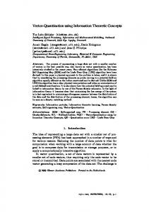
Figure 2 : Experimental (thin curves) and modelled (thick curves) bit rates B (bits/min) vs. V (classif./min.) for best users (plain curves) and worst users (dashed curves) of Farwell & Donchin, 1988 (a), Donchin et al., 2000 (b), Anderson & Sijercic, 1996 (c), Polikoff et al, 1995 (d). The BCI from (Farwell & Donchin, 1988) uses a 36 keys virtual keyboard controlled by P300 waves. The error on one trial Q varies from 0.71 for the best user (subject 3) to 0.77 for the worst user (subject 4). The predicted bit rate mode is sub-optimal for user 4, and at the limit between optimal and suboptimal for user 3 (the difference (aexp-alim)/aexp is only 4%), see Figure 2a. The maximum achievable predicted bit rate is 19.3 bits/minute for the best user, instead of 18.1 bits/minute according to the reported experimental data. The BCI from (Donchin et al., 2000) is a new version of the one from (Farwell & Donchin, 1988). The error on one trial Q varies from 0.67 for the best user (able-bodied) to 0.76 for the worst user (disabled). The predicted bit rate mode is optimal for disabled users, and at the limit between optimal and sub-optimal for able-bodied users (the difference (aexp-alim)/aexp is only 8%), see Figure 2b. The maximum achievable predicted bit rate is 25.1 bits/minute for the best user, instead of 24.6 bits/minute according to the reported experimental data. The BCI from (Anderson & Sijercic, 1996) uses an asynchronous protocol with bloc overlapping over time, with N=5. An average over several blocs is performed. The error on one trial vary from 0.46 for the best user (subject 1) to 0.70 for the worst user (subject 2). The predicted bit rate mode cannot be calculated, maybe because of the bloc overlapping protocol/feature used, see Figure 2c. The maximum achievable predicted bit rate is 99.6 bits/minute for the best user, instead of 48.3 bits/minute according to the reported experimental data. The BCI from (Polikoff et al., 1995) uses P300 waves and a simple protocol with N=4. The error on one trial Q is 0.52. The predicted bit rate mode is sub-optimal, which corresponds to the remark of Polikoff et al. that the average trial protocol is not efficient (true in this specific case, but not in general), see Figure 2d. The maximum achievable predicted bit rate is 6.0 bits/minute, instead of 2.7 bits/minute according to the reported experimental data.
5
Discussion and conclusions
The limit condition between optimal and sub-optimal modes allows to predict in which mode the bit rate curve will be. When designing a BCI, determining this condition allows to decide between
two options: (a) if the mode is sub-optimal the BCI should be redesigned, for instance by avoiding the use of average trial protocols; (b) if the mode is optimal, one can determine Vopt and tune the protocol accordingly. It has been observed however that this condition is not always precise enough : differences of less than 10% between the experimental and limit gradients can lead to a wrong prediction. In some other cases (e.g. Anderson & Sijercic, 1996), the operating mode cannot be predicted. This study brings some responses to the bit rate maximization question. The comparison between four BCI's showed that a high classification speed leads to a high bit rate, since in Equation 4 an increase of V induces a decrease of R, but V increases faster than R decreases which leads to an increased bit rate. In conclusion, we showed that the optimal bit rate mode can be obtained under the hypothesis that the user can emit the same mental state several times. Assuming that the BCI can operate in optimal bit rate mode, (a) such average trial protocols allow to increase the bit rate, and (b) the optimal V leading to the best B can be predicted to some extent (the inter-user variability, see Figure 2, is not taken into account in our model). Current work aims at refining this model and at validating it with more published experiments.
References Anderson, C. W., & Sijercic, Z. (1996). Classification of EEG signals from four subjects during five mental tasks. In A.B. Bulsari, S. Kallio & D. Tsaptsinos, (Eds.), Solving Eng. Problems with Neural Networks, Proc. Conf. Eng. App. in neural networks (EANN'96), 407-414. Bayliss, J. D. (2001). A flexible brain-computer interface. PhD Thesis, Dpt. Comp. Sc., Univ. Rochester, NY. Donchin, E., Spencer, K. M., & Wijesinghe, R. (2000). The mental prosthesis: assessing the speed of a P300-based brain–computer interface. IEEE Trans. Rehab. Eng., 8, 2, 174-179. Farwell, L.A. & Donchin, E. (1988). Talking off the top of your head: toward a mental prosthesis utilizing event-related brain potentials, Electroen. and Clin. Neuro., 70, 510-523. Lehtonen, J. (2002). EEG-based brain computer interfaces. M.Sc. Thesis, Dpt. of Electr. and Comm. Eng., Helsinki University of Technology, Retrieved from http://www.lce.hut.fi/. Millán, J. del R., Mouriño, J., Babiloni, F., Cincotti, F., Varsta, M. & Heikkonen, J. (2000). Local neural classifier for EEG-based recognition of mental tasks. IEEE-INNS-ENNS Int. Joint Conf. on Neural Networks (IJCNN 2000), 3, 632 –636. Como, Italy. Polikoff, J. B., Bunnell, H. T. & Borkowski, W. J., Jr. (1995), Toward a P300-based computer interface. Proc. Rehab. Eng. and Assistive Technology Society of North America (RESNA'95), 178-180. Arlington, Va: RESNAPRESS Renkens, F. & Millán, J. del R. (2002). Brain-actuated control of a mobile platform, Int. Conf. Simulation of Adaptive Behavior, Workshop Motor Control in Humans and Robots, Edinburgh. Wolpaw, J. R., Ramoser, H., McFarland, D. J. & Pfurtscheller, G. (1998). EEG-based communication: improved accuracy by response verification. IEEE Trans. Rehab. Eng., 6, 3, 326-333.
6
Annex A – Simplified bit rate definitions
The bit rate definition from Equations 1 to 3 can be simplified in some manner. Two simplifications has been proposed, one by Farwell & Donchin, 1988 and the another by Wolpaw et al. in 1998. Farwell & Donchin assume that the classifier is without rejection (M=N) and is perfect (i.e. no classification error), therefore the transition matrix p(yj|xi)=I, with I the identity matrix of size NxN. The mental states are assumed to be equiprobable, therefore p(xi)=1/N. We have so : N N N 1 1 1 p ( y j ) = ∑ p ( xi ) ⋅ p ( y j xi ) = ∑ ⋅1 + ∑ ⋅ 0 = N i =1 i= j N i≠ j N 1 424 3 0
H ( y ) = −∑ p ( y j ) ⋅ log 2 p ( y j ) = −∑ M
M
j =1
j =1
1 1 1 1 ⋅ log 2 = − N ⋅ log 2 = log 2 N N N N N
N,N N ,N 1 1 H cond ( y x ) = −∑∑ p ( xi ) ⋅ p ( y j xi ) ⋅ log 2 p ( y j xi ) = − ∑ ⋅ 0 ⋅ log 2 0 − ∑ ⋅1⋅ log 2 1 = 0 N N i =1 j =1 i= j i= j 144244 3 14 4244 3 N
M
(
=0
)
B = V ⋅ H ( y ) − H cond ( y x ) = V ⋅ log 2 N
=0
[bits/second]
Wolpaw et al assume that the classifier is without rejection (M=N), that the accuracy p(yi|xi) is constant (p(yj|xi)=P) and that the classification error (1-P) is distributed equally on other classes ((1-P)/(N-1) for each class). The mental states are assumed to be equiprobable, therefore p(xi)=1/N. if i = j
P p ( y j xi ) = 1 − P N − 1
else
p ( y j ) = ∑ p ( xi ) ⋅ p ( y j xi ) = ∑ N
N
i =1
i= j
N 1 1 1− P P 1 1− P P 1− P 1 ⋅P+∑ ⋅ = + ( N − 1) ⋅ ⋅ = + = N N N N −1 N N N i≠ j N N −1 14243 0
H ( y ) = −∑ p ( y j ) ⋅ log 2 p ( y j ) = −∑ M
M
j =1
j =1
1 1 1 1 ⋅ log 2 = − N ⋅ log 2 = log 2 N N N N N
H cond ( y x ) = −∑∑ p ( xi ) ⋅ p ( y j xi ) ⋅ log 2 p ( y j xi ) = N
M
i =1 j =1
=− =−
1 N
∑∑ p ( y
1 N
∑1⋅ P ⋅ log
N
xi ) ⋅ log 2 p ( y j xi ) =
N
i =1 j =1
j
N
i =1
2
P + ( N − 1) ⋅
1− P 1− P ⋅ log 2 = N −1 N −1
1 1− P = − ⋅ N ⋅ P ⋅ log 2 P + (1 − P ) ⋅ log 2 = N N −1 1− P = − P ⋅ log 2 P − (1 − P ) ⋅ log 2 N −1
1− P B = V ⋅ H ( y ) − H cond ( y x ) = V ⋅ log 2 N + P ⋅ log 2 P + (1 − P ) ⋅ log 2 [bits/second] N −1 In this paper, we use Wolpaw et al simplification because it is very simple and most of published experiments provide the classification speed V, the accuracy P and the number of classes N.
(
7
)
Annex B – Average-trial protocol model
Assuming that Wolpaw et al definition of bit rate is used, we know that the classification error on a single trial will be Q=1-P1, with P1 the accuracy for a single-trial. Then, the classification error for k successive trials will be (assuming that the user emit the same mental state k successive times and that the classification error Qi is constant over time) : k
k
i =1
i =1
Qk = ∏ Qi ; ∏ Q = Q k
If we also assume that (a) averaging k successive trials then classifying, and (b) classifying k trials then averaging leads to the same model, we can write : Pk=1-Qk
8
Annex C – Classification speed for the maximum bit rate
The maximum bit rate is obtained when the derivative of B is equal to zero (dB/dV=0). We will calculate this derivative and the solution of that equation will give us the maximum classification speed that leads to the maximum bit rate. We use the simplified bit rate definition from (Wolpaw, 1998), see Annexe A. The accuracy is given by our model (Equation 5). Since we known that k=1/(V⋅t1), we can write Equation 4 as : 1 1 1 1 V ⋅t Q V ⋅t V ⋅t V ⋅t B = V ⋅ log 2 N + 1 − Q ⋅ log 2 1 − Q + Q ⋅ log 2 = N − 1 1
1
1
1
1
1 1 1 Q V ⋅t1 s = V ⋅ log 2 N + V ⋅ 1 − Q V ⋅t1 ⋅ log 2 1 − Q V ⋅t1 + V ⋅ Q V ⋅t1 ⋅ log 2 1424 3 N −31 14442444 X 144444244444 3 Z Y
We can see that this equation vary only respect to the classification speed V and depends on some constants values (N, t1, Q). The bit rate definition is decomposed in a sum of products so the derivative will be easier to calculate : dB = X ′ + Y′+ Z′ dV
Derivative of X : Derivative of Y :
X ′ = log 2 N
Y′: 1 1 Y = V ⋅ 1 − Q V ⋅t1 ⋅ log 2 1 − QV ⋅t1 4244 244 14 3 144 3 v1
u1
v1 = V{ ⋅ 1 − Q v2 1424 3 1 V ⋅t1
u2
Y ′ = u1′ ⋅ v1 + u1 ⋅ v2′
1 u1 = log 2 1 − QV ⋅t1 1424 3 u2
1 ′ 1 ′ V1⋅t ′ 1 − Q V ⋅t1 1′ − Q V ⋅t1 Q 1 ′ u = = − u1′ = log ( u2 ( x ) )′ = 2 = 1 1 1 u2 V ⋅t1 V ⋅t 1 V ⋅t1 1− Q 1− Q 1− Q 1 1 ′ v1′ = ( v2 ⋅ u2 )′ = u2′ ⋅ v2 + u2 ⋅ v2′ = − Q V ⋅t1 ⋅ V + 1 − Q V ⋅t1 V1⋅t ′ Q 1 1 1 1 V1⋅t ′ V ⋅t1 V ⋅t1 V ⋅t1 Y′ = − ⋅V ⋅ 1 − Q + log 2 1 − Q ⋅ 1 − Q − Q 1 ⋅V = 1 V ⋅t1 1− Q
1 1 1 ′ 1 ′ = − QV ⋅t1 ⋅V + log 2 1 − Q V ⋅t1 ⋅ 1 − QV ⋅t1 − QV ⋅t1 ⋅ V Derivative of Z : Z′ : Z = v3 ⋅ u3 Z ′ = u3′ ⋅ v3 + u3 ⋅ v3′ 1 1 V ⋅t1
v3 = V{ ⋅ Q { v2
u4
QV ⋅t1 u3 = log 2 = log 2 Q V ⋅t1 − log 2 ( N − 1) N −1
V1⋅t ′ Q 1 u4′ u3′ = log ( u4 ( x ) ) = = 1 u4 QV ⋅t1 1 1 ′ v3′ = v2′ ⋅ u4 + v2 ⋅ u4′ = Q V ⋅t1 + V ⋅ Q V ⋅t1
1
V1⋅t ′ 1 Q 1 1 1 V ⋅t1 V1⋅t ′ Q V ⋅t1 V ⋅t1 1 ⋅ V ⋅ Q + log 2 ⋅ Q +V ⋅ Q = Z′ = 1 N − 1 V ⋅t1 Q 1 V1⋅t ′ V1⋅t ′ Q V ⋅t1 V ⋅t1 1 1 = Q ⋅ V + log 2 ⋅ Q +V ⋅ Q N − 1 1
Derivative of B : 1 1 1 V1⋅t ′ V1⋅t ′ Q V ⋅t1 V ⋅t1 V ⋅t1 V ⋅t1 1 1 B′ = log 2 N + log 2 1 − Q ⋅ 1 − Q − Q ⋅V + log 2 ⋅ Q +V ⋅Q = N − 1 1
1 1 1 1 ′ = log 2 N + log 2 1 − Q V ⋅t1 ⋅ 1 − Q V ⋅t1 − Q V ⋅t1 ⋅ V ⋅ log 2 1 − Q V ⋅t1 + 1 1 ′ Q V ⋅t1 Q V ⋅t1 log 2 ⋅ Q V ⋅t1 + log 2 ⋅ V ⋅ Q V ⋅t1 N −1 N −1 1
1
1
1 1 1 Q V ⋅t1 = log 2 N + 1 − Q V ⋅t1 ⋅ log 2 1 − Q V ⋅t1 + Q V ⋅t1 ⋅ log 2 + N −1 1 1 V ⋅t1 V1⋅t ′ Q V ⋅t1 1 − log 2 1 − Q Q ⋅ V ⋅ log 2 N −1 1 ′ 1 1 B V ⋅t1 Q V ⋅t1 V ⋅t1 = + Q ⋅ V ⋅ log 2 − log 2 1 − Q V N −1 f ( x) ′ f ( x) derivative property : a = − ln a ⋅ f ′( x) ⋅ a
(
)
1 V1⋅t ′ 1 ′ Q 1 =( a f ( x ) ) = − ln Q ⋅ 2 ⋅ Q V ⋅t1 V ⋅ t1 1 1 1 B 1 Q V ⋅t1 V ⋅t1 B′ = − ln Q ⋅ 2 ⋅ Q ⋅V ⋅ log 2 − log 2 1 − Q V ⋅t1 = V V ⋅ t1 N −1 1 1 1 B 1 Q V ⋅t1 = − ln Q ⋅ ⋅ QV ⋅t1 ⋅ log 2 − log 2 1 − Q V ⋅t1 V V ⋅ t1 N −1
To simplify this equation2, we will make a variable substitution : 1
1 1 1 QV ⋅t1 V ⋅t1 V ⋅t1 V ⋅t1 ′ B = log 2 N + 1 − Q ⋅ log 2 1 − Q + Q ⋅ log 2 N −1
− ln Q
1 V ⋅t1
⋅Q
1 V ⋅t1
1 1 QV ⋅t1 V ⋅t1 ⋅ log 2 − log 2 1 − Q N −1
w = log 2 N + (1− w − w ⋅ ln w ) ⋅ log 2 (1 − w ) + ( w − w ⋅ ln w ) ⋅ log 2 N −1
with
w=Q
1 V ⋅t1
The equation B'=0 has two solutions. The first one is trivial (w=(N-1)/N) and can be found by hand, but unfortunately this solution doesn't exist because the corresponding speed is greater than the maximum classification speed that can be delivered by the experiment protocol. The second one is too complex to be calculated analytically but it can be estimated numerically. As this last equation vary with two parameters N and w, we will fix the value of N then solve numerically the equation with w unknown. The founded value of w will allow us to calculate the optimal classification speed. To avoid the need to solve that equation for each N, we calculate a lot of solutions for different N then made a curve fitting : 0.9 0.8 0.7
w [-]
0.6 0.5
w opt log(N)*0.8/3
0.4 0.3 0.2 0.1 0 0
200
400
600
800
1000
N [-]
As the number of classes N is relatively low (less than 10) in BCI, we choose to have a good approximation of w between 2 and 50, and a less accurate approximation for N>50. So the w that leads to a null derivative can be approximated by : wˆ ( N ) =
8 ⋅ log N 30
∀ N ∈ {2;50}
From this definition, we can calculate the optimal classification speed : 1 log Q w = Q V ⋅t1 ⇒ V = t1 ⋅ log w
2
This derivative has been verified with Maple 8 and numerically (∆B/∆V, for N=5, Q=0.4, t1=2).
B (V ) = Bmax
⇔
Vopt ;
log Q 8 t1 ⋅ log ⋅ log N 30
Please note that the error on the classification speed V (due to the approximation wˆ ) has not been calculated. This optimal classification speed has been tested to be working for some experimental data (Polikoff et al, 1995, Farwell et Donchin, 1988, Donchin et al, 2000), but non working for (Anderson, 1996), maybe because the protocol is using block overlapping. Further analysis will be necessary to explain that. Using this definition of Vopt, we can calculate the optimal number of trials kopt and the optimal accuracy Pkopt. With theses two definitions, it is possible to calculate the bit rate using the definition (Equation 4).
kopt
Popt = 1 − Q
k opt
⇒ log (1 − Popt ) = log Q ⇒ Popt = 1 −
9
8 log ⋅ log N 1 30 = ; Vopt ⋅ t1 log Q
k opt
; log Q
8 log ⋅log N 30 log Q
8 log ⋅ log N 30 log Q = log 8 ⋅ log N = log Q 30
8 ⋅ log N 30
Annex D – Determining the bit rate operating mode
To determine whether or not the bit rate curve will be in optimal operating mode (Equations 9 and 10), we will calculate its slope (=derivative) in the vicinity of the maximum classification speed, see Figure 1b. If the slope is positive, then the bit rate will be in sub-optimal mode. If the slope is negative, the bit rate will be in optimal mode. Let's calculate the derivative of B respect to V : 1− P B = V ⋅ log 2 N + P ⋅ log 2 P + (1 − P ) ⋅ log 2 N −4 1 14444444 424444444 3 R
dB dR = R+ V ⋅ dV dV P varies implicitly with N, so we need to derive R respect to V. We can also write : dR dR dP dk = ⋅ ⋅ dV dP dk dV with
dR 1 − P ′ = ( P ⋅ log 2 P )′ + (1 − P ) ⋅ log 2 dP N −1 1 1 1 1− P + 1 ⋅ log 2 P + (1 − P ) ⋅ ⋅ − + ( −1) ⋅ log 2 1 − P N − 1 P N −1 N −1 1− P = log 2 P − log 2 N −1 = P⋅
and k=
1 1 = ⋅ V −1 V ⋅ t1 t1
dk 1 1 = − ⋅ V −2 = − dV t1 t1 ⋅ V 2 dP/dk is the experimental slope of the accuracy. It can be calculated in the vicinity of the maximum classification speed (which corresponds to k=1) : dB dR dP dk = 0 = R+V ⋅ ⋅ ⋅ dV k =1 dP dk dV k =1 1 − P dP 1 = R + V ⋅ log 2 P − log 2 ⋅− ⋅ 2 1 N − dk t ⋅ 1 V = R+
k =1
1− P dP ⋅ − log 2 P + log 2 dk N −1
1− P log 2 N + P ⋅ log 2 P + (1 − P ) ⋅ log 2 dP R N −1 = a ⇒ = = lim 1 1 − P − P dk log P − log log 2 P − log 2 2 2 N −1 N −1 with P=P1 (accuracy for k=1). If the experimental initial slope of P is higher than alim, then the bit rate curve will be in optimal mode.
This limit can be simplified : alim =
log 2 N + P1 ⋅ log 2 P1 + (1 − P1 ) ⋅ log 2
1 − P1 N −1
1 − P1 N −1 1 − P1 1 − P1 log 2 N + P1 ⋅ log 2 P1 + log 2 − P1 ⋅ log 2 N −1 N −1 = 1 − P1 log 2 P1 − log 2 N −1 1 − P1 log 2 N + log 2 N −1 = P1 + 1 − P1 log 2 P1 − log 2 N −1 log 2 P1 − log 2