On P Systems with Promoters/Inhibitors Mihai IONESCU Research Group on Mathematical Linguistics Rovira i Virgili University Pl. Imperial T´arraco 1, 43005 Tarragona, Spain E-mail:
[email protected] Drago¸s SBURLAN Department of Computer Science Ovidius University of Constant¸a Bd. Mamaia 124, Constant¸a, Romˆania E-mail:
[email protected] Abstract. This article shows how the computational universality can be reached by using P systems with object rewriting context-free rules, promoters/inhibitors and one catalyst. Both generative and accepting cases are studied. Some examples that illustrate the theoretical issues are also presented.
1
Introduction
P systems represent a class of distributed/parallel computing devices whose functioning is inspired from the behavior of molecules and living cells. There, chemical compounds are processed in a massive parallel manner inside a compartmental structure of membranes that control the substances exchanges between regions they delimit. The reactions that take place inside such a biological structure can be formally described by cooperative rules. One particular case is that of catalytic rules which model the biological reactions that can take place only with the help of certain enzymatic proteins (which participate in reactions and remain unmodified after they occur). Another important type is that of promoted/inhibited reactions that happen in the presence/absence of certain chemicals which are not directly implied in reactions. In this abstract, symbolic, mathematical framework it is interesting to see which is the computational power when “low” cooperation features are used. In this sense, as it was shown in [4], P systems with context-free and catalytic rules with only two distinct catalysts are computational universal. Also, in [1] a model with context-free rules, one catalyst and promoters at the level of rules s shown to be universal. In this paper we explore the computational power of the systems with context-free rules, catalytic rules with one catalyst and promoters/inhibitors. Both generative and accepting cases will be studied here. Meanwhile, we introduce the regulated rewriting mechanism of regularly controlled context-free grammars for as a tool in the study of P systems.
264
2
Preliminaries
2.1
Regulated Rewriting
In any Chomsky grammar, at some given step in a derivation one can use for rewriting any applicable rule in any desired place of the sentential form. In order to restrict this nondeterminism some regulating mechanisms, which can control the derivation process, were considered. Using such regulations we can arrive to computational universality even if we use context-free grammars as a core generative device. In literature there are many types of regulations which restrict the use of rules in a Chomsky grammar (see [3], [8]). Here we will present only regularly controlled grammars with appearance checking and λ–rules. A regularly controlled context-free grammar with appearance checking is a 6-tuple GrC = (N, T, P, S, R, F ) where N ,T ,P , and S are specified as in context-free grammar, R is a regular language over P , and F is a subset of P . For a rule p = A → w ∈ P and x, y ∈ VG∗ we write x =⇒ac p y if either 1. x = x1 Ax2 and y = x1 wx2 , or 2. x = y, A does not appear in x, and p ∈ F . The language L(G) generated by G with appearance checking consists of all words w ∈ T ∗ such that there is a derivation ac ac S =⇒ac p1 w1 =⇒p2 w2 · · · =⇒pn wn = w
with p1 p2 · · · pn ∈ R. We say that G is a regularly controlled grammar without appearance checking iff F = ∅. By L(λrC), L(λrCac ), L(rC), and L(rCac ) we denote the families of languages generated by regularly controlled grammars (without appearance checking), regularly controlled grammars with appearance checking, regularly controlled grammars without erasing rules (and without appearance checking), and regularly controlled grammars with appearance checking and without erasing rules, respectively. The following results stand: L(CF ) ⊂ L(rC) ⊆ L(λrC) ⊂ L(λrCac ) = L(RE). Interesting for the scope of the present paper is the last equality, L(λrCac ) = L(RE), since we will simulate a regularly controlled grammar with appearing checking and λ–rules with P systems in order to show their universality.
2.2
Register Machines
We will use in our paper the power of Minsky’s register machine [6], that is why we recall here this notion. Such a machine runs a program consisting of numbered instructions of several simple types. Several variants of register machines with different number of registers and different instructions sets were shown to be computationally universal (see [6] for some original definitions and [5] for the definition we use in this paper). A n-register machine is a construct M = (n, P, i, h), where: 265
• n is the number of registers, • P is a set of labeled instructions of the form j : (op(r), k, l), where op(r) is an operation on register r of M , and j, k, l are labels from the set Lab(M ) (which numbers the instructions in a one-to-one manner), • i is the initial label, and • h is the final label. The machine is capable of the following instructions: (add(r), k, l) : Add one to the contents of register r and proceed to instruction k or to instruction l; in the deterministic variants usually considered in the literature we demand k = l. (sub(r), k, l) : If register r is not empty, then subtract one from its contents and go to instruction k, otherwise proceed to instruction l. halt : This instruction stops the machine. This additional instruction can only be assigned to the final label h. A deterministic m-register machine can analyze an input (n1 , ..., nα ) ∈ Nα0 in registers 1 to α, which is recognized if the register machine finally stops by the halt instruction with all its registers being empty (this last requirement is not necessary). If the machine does not halt, the analysis was not successful.
2.3
P Systems Prerequisites
A P system (of degree m ≥ 1) with symbol–objects and rewriting evolution rules is a construct Π = (V, C, µ, w1 , . . . , wm , (R1 , ρ1 ), . . . , (Rm , ρm ), i0 ), where: • V is the alphabet of Π; its elements are called objects; • C ⊆ V is the set of catalysts; • µ is a membrane structure consisting of m membranes labeled 1, 2, · · · , m; • wi , 1 ≤ i ≤ m, specify the multisets of objects present in the corresponding regions i at the beginning of a computation; • Ri , 1 ≤ i ≤ m, are finite sets of evolution rules over V associated with the regions 1, 2, . . . , m of µ, and ρi is a partial order relation over Ri (a priority relation); these evolution rules are of the form a → v or ca → cv, where a is an object from V − C and v is a string over (V − C) × ({here, out, in}) (In general, the target indications here, out, in are written as subscripts of objects from V .); • i0 is a number between 0 and m and specifies the output membrane of Π (in case of 0, the environment is used for the output). 266
Starting from the original model some variants were proposed (see [7]). One of them is P systems with promoters/inhibitors and was introduced in [1]. In the case of promoters, the rules (reactions) are possible only in the presence of certain symbols. An object a is a promoter for a rule u → v, and we denote this by u → v|a , if the rule is active only in the presence of object a. An object b is an inhibitor for a rule u → v, and we denote this by u → v|¬b , if the rule is active only if inhibitor b is not present in the region. In particular, promoters/inhibitors themselves can evolve according to some rules. The difference between catalysts and promoters consists in the fact that the catalysts directly participate in rules (but are not modified by them), and they are counted as any other objects, so that the number of applications of a rule is as big as the number of copies of the catalyst, while in the case of promoters, the presence of the promoter objects makes it possible to use the associated rule as many times as possible, without any restriction; moreover, the promoting objects do not necessarily directly participate in the rules. As a consequence, one can notice that the catalysts inhibits the parallelism of the system while the promoters/inhibitors only guide the computation process. The P system with the mentioned features starts to evolve from an initial configuration, by performing all operations in a parallel way, for all applicable rules, for all occurrences of objects in the region associated with the rules, for all regions at the same time and according to a universal clock. A computation is successful if and only if it halts, meaning that no rule is applicable to the objects present in the final configuration. The result of a halting computation is the number of objects present in the region i0 in the halting configuration. The set of all numbers constructed in this way by a system Π is denoted by N (Π). For such kind of P systems we will use the following notation: N OPm (α, β), α ∈ {ncoo, coo} ∪ {catk | k ≥ 0}, β ∈ {proR, inhR} to denote the family of sets of natural numbers generated by P systems with at most m membranes, evolution rules that can be non-cooperative (ncoo), cooperative (coo), or catalytic (catk ), using at most k catalysts, and promoters (proR) or inhibitors (inhR) at the level of rules. Also, we may consider as the result of a halting computation the vector Ψ(w) (the vector of multiplicities of objects) where w is the multiset present in the region i0 in the halting configuration. In this case, the set of all vectors constructed in this way by a system Π is denoted by P s(Π). We will use also the following notation: P sIPm (α, β), α ∈ {ncoo, coo} ∪ {catk | k ≥ 0}, β ∈ {proR, inhR}, to denote the family of sets of vectors of natural numbers generated by P systems with at most m membranes, evolution rules that can be non-cooperative (ncoo), cooperative (coo), or catalytic (catk ), using at most k catalysts, and promoters (proR) or inhibitors (inhR) at the level of rules. Here, I stands for P systems with internal input. In this paper we will show how the regularly regulated context-free grammars with appearance checking can be used to prove the computational universality of such type of P systems. Also we will also study the deterministic P systems accepting sets of vectors of natural numbers. We indicate [1] for more details concerning P systems with promoters/inhibitors.
267
' ' '
0 → 0out 1 → 1out 1 & &
$
c $ 0
0 → 0 Aout c00 → c0out 1 → 10 10 → 100 Bout % c100 → c1out 2
&
A → A0 0 → 0out |A0 $ A0 → A00 0 → λ|A00 A00 → λ B → B0 1 → λ|B 0 B 0 → B 00 1 → 1out |B 00 % B 00 → λ 3
%
Figure 1: Simulation of the AND gate using promoters and one catalyst
3
Some Relevant Examples
In this section we will present some examples of P systems computing some “sensitive” tasks using above introduced types of P systems. First we will construct a P system with promoters that, having as input two values, say 0 and/or 1, computes the and operation (see Figure 1). Formally, we define the following P system ΠAN D = (V, C, µ, w1 , w2 , w3 , R1 , R2 , R3 , 0), where: •
V = {0, 1, 00 , 10 , 100 , A, A0 , A00 , B, B 0 , B 00 , c};
•
C = {c};
•
µ = [3 [2 [1 ]1 ]2 ]3 ;
•
w1 = w3 = ∅, w2 = {c};
•
R1 = {1 → 1out , 0 → 0out }; R2 = {0 → 00 Aout , c00 → c0out , 10 → 100 Bout , 1 → 10 , c100 → c1out }; R3 = {A → A0 , 0 → 0out |A0 , A0 → A00 , 0 → λ|A00 , A00 → λ, B → B 0 , 1 → λ|B 0 , B 0 → B 00 , 1 → 1out |B 00 , B 00 → λ}.
The simulation of the AND gate uses the catalyst c to inhibit the parallelism and to separate the entrance time of objects 0 and 1 into region 3. According to the entrance time, objects will be either deleted, or sent out into the environment. More specifically, if we consider that initially we had two objects 0 inside region 2, the rule 0 → 00 Aout is executed. Its role is to introduce the object A into region 3 to set up the “right” configuration of the region. Next, in region 2 the only applicable rule is c00 → c0out , which will introduce one object 0 into region 3. At the same time, in region 3 the rule A → A0 is executed. Now, we 268
'
'
c, an , bm
2 &
$ $
ca → ca0 d|¬a0 cb → cb0 d|¬b0 a0 → Aout |¬b b0 → Bout |¬a d→λ 1 a0 → λ|¬d b0 → λ|¬d & % %
Figure 2: Integer subtraction using inhibitors and one catalyst
will have in region 3 the objects A0 and 0, and the rules that will be applied are 0 → 0out |A0 and A0 → A00 . These rules guarantee that an object 0 is sent out into the environment. In the meantime, in region 2, the remaining object 00 reacts with the catalyst c and an object 0 will be introduced into region 3 (the rule used is again c00 → c0out ). Here, the object 0 will find a different context since now, in region 3 there is no object A0 . Therefore, the rules 0 → λ|A00 and A00 → λ are applied, hence the initial configuration of the system is restored. Basically, a similar method stands for the other cases, with some minor changes: objects 1 enter into region 3 with one computational delay (because of the rule 1 → 10 present in region 2) in order not to influence the processes executing in region 3; the first object 1 that enters into region 3 is deleted (as opposed to the above case when the first object 0 that arrives in region 3 is sent out) by using the rule 1 → λ|B 0 . Recall that the membrane 1 can be entirely avoided, its role being only to specify the entry point of the input. Also, the result of computation is sent out into environment even if it is actually obtained in region 3. This features are useful when we want to connect gates into circuits (see [2] for more details). The second example (see Figure 2) uses context-free rules, inhibitors and one catalyst to compute the arithmetic difference between the initial multiplicity of two distinct objects, present at the beginning of computation into an “input” region. Formally, we define the following P system Πsubtraction = (V, C, µ, w1 , w2 , R1 , R2 , 2), where: •
V = {a, b, a0 , b0 , d, A, B, c};
•
C = {c};
•
µ = [2 [1 ]1 ]2 ;
•
w1 = {c, an , bm }, w2 = ∅;
•
R1 = {ca → ca0 d|¬a0 , cb → cb0 d|¬b0 , a0 → Aout |¬b , b0 → Bout |¬a , d → λ, a0 → λ|¬d , b0 → λ|¬d }; R2 = ∅.
269
The system starts the computation having into the input membrane 1 a catalyst c and the objects an , bn , whose multiplicity we want to subtract. The result of computation is sent to region 2 and it is represented by: • An−m if n > m; • B m−n if m > n; • no object is sent to region 2 meaning that m = n. The system works as follows: while there are still objects a and b, they are deleted in pairs, iteratively, up to a moment when there are no more objects a, for instance (or objects b). At that moment, the flow of computation changes and as a result, also iteratively, the remaining objects b (or objects a, respectively) are send out. During the computation, the promoters control the derivation process, while the catalyst inhibits the parallelism. For a better understanding we present the configuration table for the case when both objects a and b are present simultaneously into the input membrane. t0 t1 t2 t3 t00 ···
region 1 c, an , bm ca → ca0 d|¬a0 c, an−1 , bm , a0 , d cb → cb0 d|¬a0 d→λ n−1 m−1 0 0 c, a ,b ,a ,b ,d d→λ c, an−1 , bm−1 , a0 , b0 a0 → λ|¬d b0 → λ|¬d c, an−1 , bm−1 ca → ca0 d|¬a0 ···············
region 2
·········
Here we have considered only the case when at the first step an object a reacts with the catalyst c. The result of computation remains unchanged (due to symmetry reasons) even if, at the first step, an object b reacts with the catalyst c. When in the region remain only objects a, the configuration table for the forthcoming computations is: tp tp+1 t0p ···
region 1 c, ak ca → ca0 d|¬a0 c, ak−1 , a0 , d a0 → Aout |¬b0 d→λ c, ak−1 ca → ca0 d|¬a0 ···············
region 2
A ·········
The case when inside the region 1 remain only objects b and the catalyst c is similar with the previous one, and has as result the production into region 2 of m − n copies of objects B.
270
Since in both examples we have used some context-sensing features we may conjecture that both P systems with promoters and P systems with inhibitors, using only one catalyst, are computational universal. Indeed, the following section will be dedicated to these issues and, there, we will show how any recursively enumerable set of natural numbers can be obtained using these types of P systems.
4
Universality Results
4.1
Computational Universality – The Generating Case
Here, we present two universality results concerning P systems with promoters or inhibitors at the level of rules. The proofs are based on the simulations of regularly controlled context-free grammars with appearance checking for which the equivalence with RE stands. We denote by N OPm (cat, proR), the family of sets N (Π) computed by systems with at most m membranes, 1 catalyst (say c) and objects as promoters. By N RE we denote the family of Turing computable sets of numbers. Theorem 1
N OP2 (cat1 , proR) = N RE.
Proof. We will consider for this proof the implication N RE ⊆ N OP2 (cat, proR); the other way around is a long, but straightforward construction. Let Greg = (Nreg , Treg , Preg , Sreg ) be a regular grammar generating the regular set Lreg . We denote by r the number of rules in Preg . The rules of Preg are enumerated as i : (Mi → pi Qi ) or i : (Mi → pi ) with 1 ≤ i ≤ r, where Mi ∈ Nreg and pi ∈ Treg ∀ 1 ≤ i ≤ r. For any such grammar Greg we can construct an equivalent right–linear grammar G0 = (N 0 , T 0 , P 0 , S 0 ) in the following way: T 0 = Treg , S 0 = Sreg , N 0 = Nreg ∪ {M(i,1) , M(i,2) , M(i,3) | 1 ≤ i ≤ r}. P0
For any rule i : (Mi → pi Qi ) ∈ Preg or i : (Mi → pi ) ∈ Preg , 1 ≤ i ≤ r we will have in the sequence of rules: Mi → M(i,1) , M(i,1) → M(i,2) , M(i,2) → M(i,3) , M(i,3) → pi Qi , Mi → M(i,1) , M(i,1) → M(i,2) , M(i,2) → M(i,3) , M(i,3) → pi
respectively. Moreover, P 0 does not contain other rules excepting the rules considered above. In other words, the only difference between the two grammars is that the production of a new terminal in grammar G0 is done after each fourth step of a derivation. Now let us construct a P system which simulates the derivation process of a regularly controlled grammar with appearance checking. The system will use only two membranes, one catalyst and promoters. The innermost membrane will contain the generative mechanism and the results of computation will be send out to the skin membrane which will be the output membrane of the system (the reason is that the catalyst is used during the computation to inhibit the parallelism and it cannot be removed, therefore we cannot obtain the number 0 as the result of computation if we use only one membrane). In what follows 271
we will discuss only the rules in the innermost membrane since the skin membrane does not execute any task (its role is only to collect the objects obtained during computation). The promoters will be generated by a mechanism like the one presented above (promoters will be actually terminal symbols from T 0 and, therefore, they will be generated at each forth step). They will permit the execution of “context-free” rules in the “right” order – the order given by the regular mechanism. In order to correctly simulate the appearance checking mechanism we have to modify the rules in the grammar G0 such that we replace each rule of type M(i,3) → pi Qi by rules of type: M(i,3) → pi Qi f or M(i,3) → pi Qi a depending on how the object pi indicates a rule from F (in the regularly controlled grammar definition, the set F ⊂ P represents the appearance checking set of rules; we will use the object a to identify that a rule with the corresponding label pi is in the appearance checking set; if not, we will produce in the rule the object f ). We will consider also the same construction for the rules in G0 of type M(i,3) → pi , i.e., M(i,3) → pi f or M(i,3) → pi a. This means that, in the definition of our P system, for the inner membrane, we will have rules of the following types: • Mi → M(i,1) , M(i,1) → M(i,2) , M(i,2) → M(i,3) , M(i,3) → pi Qi f if pi is not a label in the appearance checking set; • Mi → M(i,1) , M(i,1) → M(i,2) , M(i,2) → M(i,3) , M(i,3) → pi Qi a if pi is a label in the appearance checking set; • Mi → M(i,1) , M(i,1) → M(i,2) , M(i,2) → M(i,3) , M(i,3) → pi f if pi is not a label in the appearance checking set; • Mi → M(i,1) , M(i,1) → M(i,2) , M(i,2) → M(i,3) , M(i,3) → pi a if pi is a label in the appearance checking set. Up to this moment, we only have considered the regular mechanism which generates labels indicating the context-free rules that should be applied. Let us denote by GCF = (NCF , TCF , PCF , SCF ) a context-free grammar with productions labeled with the elements of Treg . Now we will discuss how we can simulate (by using P systems means) the application of a context-free rule p : (A → α) indicated by the regular mechanism. For a context-free rule (p : (A → α)) ∈ GCF we will have in our P system the following sequence of rules: cA → cDα|p , p → p0 , p0 → λ|D , D → λ. Here, we have considered, without loosing the generality, that α ∈ (N ∪ Tout )∗ meaning that if we apply the rule p : (A → α) we will send to the output region the terminal symbols (recall that we are interested only in the number of objects). If promoter p, object A, and catalyst c are present at a certain moment together, then they will react only once in two consecutive computational steps. This is due to the fact that the promoter p is changed (p → p0 ) in the same moment with the execution of the rule cA → cDα|p . Moreover, the presence of the catalyst c in the rule inhibits the parallelism (we want that in one “round” the rule A → α to be applied only once and not for all occurrences of object A that may exist in the region). Now, in order to be sure that the rule cA → cDα|p was executed an object D is created; it will help to delete the object p0 present in membrane (which if not deleted can cause problems in further steps). The object D will be also deleted by the rule D → λ.
272
This sequence of rules stands for the case when the context-free rule A → α can be applied and so, it must be applied. In the case when the rule mentioned cannot be applied we have to decide if the promoter present indicates a rule with the label in the appearance checking set or not. First, let us consider the case when the promoter is not a label in the appearance checking set. In this case, recall that we deal with the following sequences of productions (from the regular mechanism): • Mi → M(i,1) , M(i,1) → M(i,2) , M(i,2) → M(i,3) , M(i,3) → pi Qi f , or • Mi → M(i,1) , M(i,1) → M(i,2) , M(i,2) → M(i,3) , M(i,3) → pi f . As the result of applying these rules we will have in the inner region, among others, the objects p and f . Let us consider that, for this case, we have the rules: f → f1 , f1 → f2 , p0 → #|f2 , f2 → λ, # → #0 , #0 → #. The first two rules from this group are meant to delay the execution of the third rule because we are not “sure” if the rule cA → cDα|p is or it is not applied. So, if the mentioned rule is applied, then the object f2 will be deleted by the rule f2 → λ and will not promote the rule p0 → #|f2 since the object p0 → λ|D was “consumed” in a previous step. As a consequence, there will be no effect (in terms of objects produced) if the previous set of rules is executed. In the opposite case (when the rule cA → cDα|p is not applied because there is no object A present in the region), then the object # will be generated. The rules # → #0 , #0 → # will cycle forever and the computation will never halt and this will mean that the computation have failed (recall that we show the universality for the nondeterministic case). With a similar construction like above we can solve the case when we deal with rules that have labels in the appearance checking set. This means that the rules to be applied are of the types: • Mi → M(i,1) , M(i,1) → M(i,2) , M(i,2) → M(i,3) , M(i,3) → pi Qi a , or • Mi → M(i,1) , M(i,1) → M(i,2) , M(i,2) → M(i,3) , M(i,3) → pi a. Here the difference from the previous case consists in not generating the trap symbol # if the rule cA → cDα|p cannot be applied. We only have to delete the promoter p0 . Its presence may interfere in the next steps of computation if it is not deleted. The rules below state the fact that if a rule is in the appearance checking set and it can not be applied even if it is indicated by the regular mechanism, then it can be skipped. a → a1 , a1 → a2 , p0 → λ|a2 , a2 → λ. Finally, the initial configuration of the P system is composed by the starting symbol SReg of the regulating mechanism, the starting symbol SCF of the context-free mechanism and the catalyst c. The system will evolve in a maximally parallel manner its behavior being controlled by the catalyst and promoters. One can notice that we arrive at the same descriptional complexity in terms of number of membranes, number of catalysts and promoters as in the original proof in [1], but 273
simulating a different computational universal mechanism.
2
As it can be seen, the promoters combined with one catalyst are sufficient to prove the computational universal capabilities of the P systems when using only context-free object rewriting rules. Also, a similar result, but concerning inhibitors instead of promoters, stands. Theorem 2
N OP2 (cat1 , inhR) = N RE.
Proof. Let us consider a similar construction like the one in the previous proof, but considering a sequence of rules as the one given below. Here we also will have two membranes and will discuss only the rules presented in the inner membrane, the skin membrane being used only to collect the result of computations. First let us recall that the rules from the context-free grammar are labeled with the symbols p1 , · · · , pk . Consider also that if in the regular grammar which controls the derivation of the context-free grammar we have a rule Mi → pj Qi , then in our simulation we will have: Mi → p1 · · · pk M(i,1) , M(i,1) → p1 · · · pk M(i,2) , M(i,2) → p1 · · · pk M(i,3) , M(i,3) → p1 · · · pj−1 pj+1 · · · pk Qi f r. Moreover, in the above construction we have considered that the label pj indicates a context-free rule which is not in the appearance checking set. As it can be seen, instead of indicating the rule with the symbol pj (meaning that the context-free rule with label pj should be applied), we have used the complementary set, i.e., p1 · · · pj−1 pj+1 · · · pk . Now, let us consider the following set of rules which simulates the behavior of the context-free mechanism: cA → CDα|¬pj , pj → λ, f → f1 , r → r1 , D → D1 , r1 → r2 |¬D , f1 → f2 , f2 → #|¬D1 , f2 → λ|¬r2 , r2 → λ, D1 → λ, # → #0 , #0 → #. The first three rules of the “regular controller” produce the symbols p1 , · · · , pk and so the rule cA → CDα|¬pj cannot be applied because always object pj will be among the mentioned objects. This means that during the first three steps in a cycle the rule cA → CDα|¬pj cannot be applied. Also, at each step we delete the objects p1 , · · · , pk by rules of type pj → λ. In the last step in a cycle, we avoid to introduce the object pj and so the rule cA → CDα|¬pj can be applied. With this occasion, we also introduce the objects f and r which are used to indicate a rule which is not in the appearance checking set. The rule cA → CDα|¬pj will modify only one (if any) occurrence of object A present in the region because of the catalyst c. Moreover in the next step of computation the 274
objects p1 , · · · , pk will be again introduced, so they will forbid the execution of any rule of type cA → CDα|¬pj . Now, coming back, we can notice that the rule cA → CDα|¬pj can be applied only if there is an occurrence of object A. Recall that this rule is not in the appearance checking set and so, if it cannot be applied, then the computations must cycle forever in order not to accept. If the rule can be applied, it has to be applied and moreover all the symbols that were produced during the computation must be deleted in order not to interfere in the next cycle. Now let us see which is the result of a computation in both cases. Consider the first case, when the rule cA → CDα|¬pj is applied. Then, in the same moment, the rules f → f1 and r → r1 are executed. In the next step the rules D → D1 and f1 → f2 can be applied. The rule r1 → r2 |¬D cannot be applied since the object D is present in the region. As an effect, the region will contain the objects D1 , f2 , and r1 . So, the only applicable rules are: D1 → λ, f2 → λ|¬r2 , and r1 → r2 |¬D . Finally, the rule r2 → λ deletes the last symbol that was created in this cycle. This means that we reestablish the initial configuration and the computation can continue. Now, consider the opposite case, when the rule cA → CDα|¬pj has to be applied (because is indicated by the regular control), but it cannot be applied (because, there is no symbol A present in the region). So, the symbol D is not released. As an effect we will have in the region the objects f1 and r1 and the rules to be applied are r1 → r2 |¬D and f1 → f2 . Next, the rules f2 → #|¬D1 and r2 → λ will be applied and so the # symbol will be created and the computation will never halt. For the rules that are in the appearance checking set we can consider for the regular mechanism rules of the following types: Mi → p1 · · · pk M(i,1) , M(i,1) → p1 · · · pk M(i,2) , M(i,2) → p1 · · · pk M(i,3) , M(i,3) → p1 · · · pj−1 pj+1 · · · pk Qi , while for the “context-free” mechanism a rule: cA → Cα|¬pj is considered. In this way, if the rule can be applied, then it will be applied and if cannot be applied, then nothing will happen and the process will continue correctly simulating the appearance checking mechanism. Another aspect one can notice is that we can generate the family of recursively enumerable sets of natural non-null numbers if we use only one membrane since we use the catalyst c which remains inside the region and it cannot be removed. 2
4.2
Computational Universality – The Deterministic Accepting Case
The following theorems show the computational universality (in their accepting variant) of P systems with object rewriting non-cooperative rules and promoters/inhibitors at the level of rules. The system we propose simulates the moves of a deterministic register machine. Moreover, the obtained P system is also deterministic. Theorem 3 P sIP2 (cat1 , proR) = P sRE.
275
Proof. In order to prove this assertion we will simulate a n–register machine M = (n, P, i, h). The contents of register j will be represented in our simulation by the multiplicity of the object aj . Formally, we define the P system Π = (V, C, [1 [2 ]2 ]1 , w1 = ∅, w2 , R1 = ∅, R2 , 1), where: V = {aj , Aj , Sj | 1 ≤ j ≤ n} ∪ {F, T } ∪ {e, e0 | (e : add(j), f ) ∈ P }∪ {e, e0 , e00 | (e : sub(j), f, z) ∈ P }, C = {c}, k w2 = {c, e, aj j , 1 ≤ j ≤ n, kj ∈ N }, and R2 is defined as follows: • for each instruction (e : add(j), f ) ∈ P , we add to R2 the rules: e → e0 Aj c → caj |Aj Aj → λ e0 → f • for each instruction (e : sub(j), f, z) ∈ P , we add to R2 the rules: e → e0 T Sj caj → cF |Sj Sj → λ e0 → e00 T → T0 e00 → f |F F →λ T 0 → T 00 e00 → z|T 00 T 00 → λ • for the instruction (h : halt) ∈ P , we add to R2 the rules: aj → #|h , 1 ≤ j ≤ n h→λ • the rule # → # is added to R2 , • no other rules are added to R2 . Here is how the system works. Initially the P system starts the computation having in its input region (region 2) the objects ak11 , · · · , aknn , the catalyst c and the label e of the first instruction of the register machine we want to simulate. The vector (k1 , · · · , kn ) represents the vector that has to be accepted by our P system. The P system starts the computation by simulating the first instruction of the register machine program. Let us suppose that the first instruction to be executed is of type (e : add(j), f ) ∈ P . Then, in region 2 the rule e → e0 Aj is executed. The object Aj indicates that the number of objects aj has to be incremented. This will be realized, in the second computational step, by the promoted evolution rule c → caj |Aj ; the rules Aj → λ and e0 → f are executed in the same time with the previous one. The first 276
rule, assures that c → caj |Aj is not executed again in one iteration (therefore, j is just incremented), while the second rule allows the P system to further simulate the instruction of the register machine indicated by label f . In the case in which a subtraction instruction (e : sub(j), f, z) ∈ P is simulated, then in region 2 the rule e → e0 T Sj is executed. Note that the object Sj stands for the subtraction command; as an effect, the rule caj → cF |Sj is executed and the number of objects aj is decreased by 1 (if it is possible, i.e. the number of objects aj is greater than 0). Meanwhile, the execution of rule Sj → λ guarantees that only one object aj was deleted from the current multiset (again, if it is possible). If everything worked fine, then the sequence of rules e0 → e00 , e00 → f |F , F → λ was executed, and the label of the next register machine instruction was generated. Otherwise (i.e. there is no objects aj in region 2) the rule caj → cF |Sj is not executed therefore the object F is not produced and the rule e00 → f |F cannot be applied. Meanwhile, the object T evolves to T 0 and then to T 00 . The last step of an iteration is when the rules e00 → z|T 00 and T 00 → λ are applied simultaneously. In conclusion, the label of the next register machine instruction has been created. The above presented simulations of the instructions, (e : add(j), f ) ∈ P and (e : sub(j), f, z) ∈ P , are iterated according to the register machine program. The simulation stops when the h label (which stands for halt instruction) is generated and no other objects aj , 1 ≤ j ≤ n are into region 2. In all other cases, the trap symbol # is generated and the computation will cycle forever. 2 Theorem 4 P sIP2 (cat1 , inhR) = P sRE. Proof. This assertion will be proved by simulating a n–register machine M = (n, P, i, h). The contents of register j will be denoted in our simulation, as in the previous theorem, by the multiplicity of the object aj . Formally, we define the P system Π = (V, C, [1 [2 ]2 ]1 , w1 = ∅, w2 , R1 = ∅, R2 , 1), where: V = {aj , Aj , Sj | 1 ≤ j ≤ n} ∪ {P, P1 , Q, Q1 , Q2 , F, F1 , F2 }∪ {e, e0 | (e : add(j), f ) ∈ P } ∪ {e | (e : sub(j), f, z) ∈ P }, C = {c}, k w2 = {c, e, aj j , 1 ≤ j ≤ n, kj ∈ N }, and R2 is defined as follows: • for each instruction (e : add(j), f ) ∈ P , we add to R2 the rules: e → e0 A1 · · · Aj−1 Aj+1 · · · An S1 · · · Sn c → caj |¬Aj Ai → λ, 1 ≤ i ≤ n Si → λ, 1 ≤ i ≤ n e0 → f A1 · · · An S1 · · · Sn
277
• for each instruction (e : sub(j), f, z) ∈ P , we add to R2 the rules: e → F(j,0) QA1 · · · An S1 · · · Sj−1 Sj+1 · · · Sn caj → cP A1 · · · An S1 · · · Sn |¬Sj Ai → λ, 1 ≤ i ≤ n Si → λ, 1 ≤ i ≤ n F(j,0) → F(j,1) A1 · · · An S1 · · · Sn Q → Q1 A1 · · · An S1 · · · Sn P → P1 A1 · · · An S1 · · · Sn Q1 → Q2 A1 · · · An S1 · · · Sn |¬P F(j,1) → F(j,2) A1 · · · An S1 · · · Sn F(j,2) → zA1 · · · An S1 · · · Sn |¬P1 P1 → λ F(j,2) → f A1 · · · An S1 · · · Sn |¬Q2 Q2 → λ • no other rules are added to R2 . As in the previous theorem we start the computation having in region 2 the objects the catalyst c and the label e of the first instruction of the register machine we want to simulate. Let us consider that an increment instruction (e : add(j), f ) ∈ P has to be simulated. Then, in our P system, the existing object e (which represents the previous instruction label) is rewritten by the rule e → e0 A1 · · · Aj−1 Aj+1 · · · An S1 · · · Sn . As it can be seen only the object Aj is missing from the right hand side of the rule. The absence of this object indicates that the number of objects aj has to be incremented. Because of this, the rule c → caj |¬Aj can be applied. Meanwhile, the rules Ai → λ, 1 ≤ i ≤ n, Si → λ, 1 ≤ i ≤ n, and e0 → f A1 · · · An S1 · · · Sn are executed. Their role is to reconfigure the system for the new instruction that has to be simulated. ak11 , · · · , aknn ,
Now, let us consider that the system receive the command to subtract one object aj from the current multiset (e → F(j,0) QA1 · · · An S1 · · · Sj−1 Sj+1 · · · Sn ). We have to consider two cases: there exists or not objects aj . If |w|aj ≥ 1 where w is the current multiset present in region 2, we can apply the rule caj → cP A1 · · · An S1 · · · Sn |¬Sj since the object Sj is missing. The rules Ai → λ, 1 ≤ i ≤ n and Si → λ, 1 ≤ i ≤ n are executed at each step of computation. The objects A1 , · · · , An , S1 , · · · , Sn are created always with only one exception – when we want to execute the instruction corresponding to the missing object. The computation continues until the rule F(j,2) → f A1 · · · An S1 · · · Sn |¬Q2 is executed and the object f indicating the next instruction is generated. In a similar way like as shown in the previous theorem proof, if |w|aj = 0 then the rule caj → cP A1 · · · An S1 · · · Sn |¬Sj is not executed. Notice that objects F(j,0) and Q are “witness” that the command to simulate the subtraction scheme was made. Similarly, the presence of object P indicates that, in region 2, was at least one object aj . In order to correctly simulate the decrement instruction we want to have the “right” missing object at the “right” time. This involves some delaying rules like F(j,0) → F(j,1) A1 · · · An S1 · · · Sn , Q → Q1 A1 · · · An S1 · · · Sn , P → P1 A1 · · · An S1 · · · Sn , F(j,1) → F(j,2) A1 · · · An S1 · · · Sn . If everything worked well the rule F(j,2) → zA1 · · · An S1 · · · Sn |¬P1 is executed and the symbol z indicating the next instruction is generated. Finally, if the h symbol is generated then computation stops and accepts the input. 2 278
5
Conclusion
As it can be seen from the proofs of first two theorems concerning promoters/inhibitors at the level of rules, the use of regularly controlled context-free grammar with appearance checking is useful to show computational universality when we are not interested in minimizing the number of promoters/inhibitors. Practically, in both proofs we have used a number of promoters/inhibitors equal with the number of terminals in the regular grammar which controls the derivation process. For the last two theorems we succeeded with a P system to simulate in a deterministic manner a deterministic register machine. There we discovered that, in case of promoted P systems, 4 ∗ n promoters are enough to recognize P sRE ∩ Nn ; in case of P systems with inhibitors, the number of inhibitors used to recognize P sRE ∩ Nn was 4 ∗ n + 3. For all theorems presented, an important aspect is that the promoters/inhibitors may react at the same time as the rules they promote/inhibit. This fact, joined with the use of one catalyst which inhibits the parallelism, makes this types of P systems computational universal. Several problems regarding this topic still remain open. In the deterministic variant of recognizing P sRE ∩ Nn there is not known which is the lower bound of symbols that, acting as promoters/inhibitors, make the P system model universal (when one catalyst is used). Also, there is not known which is the computational power of P systems with promoters/inhibitors at the level of rules when no catalyst is used. Acknowledgments. The work of the first author was supported by the FPU fellowship from the Ministerio de Educacion, Cultura y Deporte. The work of the second author was possible due to a doctoral grant from Agencia Espanola de Cooperacion Internacional, Spanish Ministry of Foreign Affairs.
References [1] P. Bottoni, C. Mart´ın-Vide, Gh. P˘aun, G. Rozenberg, Membrane Systems with Promoters/ Inhibitors, Acta Informatica, 38,10 (2002), 695–720. [2] R. Ceterchi, D. Sburlan, Simulating Boolean Circuits with P Systems, Workshop on Membrane Computing WMC-Tarragona 2003 (A. Alhazov, C. Mart´ın-Vide, G. P˘aun, eds), TR 28/03, URV Tarragona, 2003. [3] J. Dassow, Gh. P˘aun, Regulated Rewriting in Formal Language Theory, SpringerVerlag, Berlin, 1989. [4] R. Freund, L. Kari, M. Oswald, P. Sosik, Computationally Universal P sSystems without Priorities: Two Catalysts Are Sufficient, submitted 2003. [5] S. Khrisna, A. P˘aun, Three Universality Results on P Systems, Workshop on Membrane Computing WMC-Tarragona 2003 (A. Alhazov, C. Mart´ın-Vide, G. P˘aun, eds),TR 28/03, URV Tarragona, 2003, 198–206. [6] M.L. Minsky, Finite and Infinite Machines, Prentice Hall, EngleWood Cliffs, 1967. [7] Gh. P˘aun, Membrane Computing. An Introduction, Springer-Verlag, Berlin, 2002.
279
[8] Gh. P˘aun, G. Rozenberg, A Guide to Membrane Computing, Theoretical Computer Science, 287, 1 (2002), 73–100. [9] G. Rozenberg, A. Salomaa, eds., Handbook of Formal Languages, Springer-Verlag, Berlin, 1997.
280