Inhomogeneous Dependency Modelling with Time Varying Copulae

*CASE – Center for Applied Statistics and Economics Humboldt-Universität zu Berlin, Berlin, Germany ** Weierstrass Institute for Applied Analysis and Stochastics, Berlin, Germany

This research was supported by the Deutsche Forschungsgemeinschaft through the SFB 649 "Economic Risk". http://sfb649.wiwi.hu-berlin.de ISSN 1860-5664 SFB 649, Humboldt-Universität zu Berlin Spandauer Straße 1, D-10178 Berlin

SFB

649

Enzo Giacomini* Wolfgang K. Härdle* Ekaterina Ignatieva* Vladimir Spokoiny**

ECONOMIC RISK

Inhomogeneous Dependency Modelling with Time Varying Copulae

BERLIN

SFB 649 Discussion Paper 2006-075

Inhomogeneous Dependency Modelling with Time Varying Copulae Enzo Giacomini1 , Wolfgang K. H¨ardle1 , Ekaterina Ignatieva1 and Vladimir Spokoiny2

1

2

CASE – Center for Applied Statistics and Economics Humboldt-Universit¨at zu Berlin, Spandauer Straße 1, 10178 Berlin, Germany Weierstrass Institute for Applied Analysis and Stochastics Mohrenstraße 39, 10117 Berlin, Germany

Abstract Measuring dependence in a multivariate time series is tantamount to modelling its dynamic structure in space and time. In the context of a multivariate normally distributed time series, the evolution of the covariance (or correlation) matrix over time describes this dynamic. A wide variety of applications, though, requires a modelling framework different from the multivariate normal. In risk management the non-normal behaviour of most financial time series calls for nonlinear (i.e. non-gaussian) dependency. The correct modelling of non-gaussian dependencies is therefore a key issue in the analysis of multivariate time series. In this paper we use copulae functions with adaptively estimated time varying parameters for modelling the distribution of returns, free from the usual normality assumptions. Further, we apply copulae to estimation of Value-at-Risk (VaR) of a portfolio and show its better performance over the RiskMetrics approach, a widely used methodology for VaR estimation.

JEL classification: C 14 Keywords: Value-at-Risk, time varying copula, adaptive estimation, nonparametric estimation Financial support from Deutsche Forschungsgemeinschaft via SFB 649 “Economic Risk” is gratefully acknowledged. 1

1

Introduction

Time series of financial data are high dimensional and have typically a non-gaussian behavior. The classical linear modelling therefore fails to reproduce the stylized facts (i.e. fat tails, asymmetry), Granger (2003). A correct understanding of the time varying multivariate (conditional) distribution is vital to many standard applications in finance: portfolio selection, option pricing, asset pricing models, Value-at-Risk (VaR) etc. The dependency (over time) of asset returns is especially important in risk management since the profit and loss (P&L) function determines the Value-at-Risk. More precisely, Value-at-Risk of a portfolio is determined by the multivariate distribution of risk factor increments. If w = (w1 , . . . , wd )> ∈ Rd denotes a portfolio of positions on d assets and St = (S1,t , . . . , Sd,t )> a nonnegative random vector representing the prices of the assets at time t, the value Vt of the portfolio w is given by Vt =

d X

wj Sj,t .

j=1

The random variable Lt = (Vt − Vt−1 ), Sj,0 = 0

(1.1)

called profit and loss (P&L) function, expresses the change in the portfolio value between two subsequent time points. Defining the log-returns Xt = log St − log St−1 , (1.1) can be written as

Lt =

d X

wj Sj,t−1 {exp(Xj,t ) − 1} .

(1.2)

j=1

The distribution function of Lt is given by Ft,Lt (x) = Pt (Lt ≤ x). The Value-at-Risk at level α from a portfolio w is defined as the α-quantile from Ft,Lt : −1 V aRt (α) = Ft,L (α). t

2

(1.3)

Copula parameter theta

4 3.5 3

theta

2.5 2 1.5 1 0.5 0 2001

2002

2003

2004

2005

time

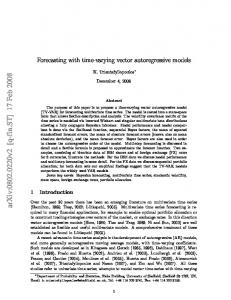
Figure 1: Dependence over time for DaimlerChrysler, Volkswagen, Bayer, BASF, Allianz and M¨ unchener R¨ uckversicherung, 20000101-20041231. It follows from (1.2) and (1.3) that Ft,Lt depends on the specification of the d-dimensional distribution of the risk factors Xt . Thus, modelling their distribution over time is essential to obtain the quantiles (1.3). The RiskMetrics technique, a widely used methodology for VaR estimation assumes that the logreturns follow a multivariate normal distribution. Here L(Xt ) = Nd (0, Σt ) a d− dimensional multivariate distribution. A more general approach is based on copulae which avoids the procrustes bed of a normality assumptions resulting in better fits of the empirical characteristics (e.g. fat tails, tail dependency) of financial returns. Modelling the distribution of returns by copulae with time varying parameters, can therefore be expected to perform better. The question though is how to steer the time varying copulae parameters. This is exactly the focus of this paper. Figure 1 shows the time varying copula parameter for DaimlerChrysler, Volkswagen, Bayer, BASF, Allianz and M¨ unchener R¨ uckversicherung from 1.Jan 2000 (20000101) to 31.Dec 2004 (20041231). In contrast the “global” copula parameter is shown by a constant horizontal line. The “local” 3

choice of copula is performed via an adaptive estimation method based on Spokoiny (2007). The adaptive estimation is based on the assumption of local homogeneity: for every time point there exists an interval of time homogeneity in which the copula parameter can be well approximated by a constant. This interval is recovered from the data using local change point analysis. For a stock portfolio, we estimate copulae with time varying parameters and simulate the VaR accordingly. Backtesting underlines the improved performance of the proposed adaptive time varying copulae fitting. This paper is organized as follows: section 2 presents the basic copulae definitions and introduces modelling log-returns with copulae. Section 3 discusses the VaR and its estimation procedure and section 4 describes three possible copulae estimation procedures. The adaptive estimation and the moving window approach are presented in section 5 and in applied on simulated data in section 6. Using real data, the performance of the copula-based VaR estimation in comparison with RiskMetrics approach is evaluated by means of Backtesting in section 7.

2

A short introduction into copulae

Copula functions have a long history in probability theory and statistics: they are well known and can be found in a variety of the financial literature. The word copula first appears in Sklar (1959), although the ideas related to copulae originate in Hoeffding (1940). Since that, copula funcions have been studied in a variety of the statistics literature such as Nelsen (1998), Mari and Kotz (2001) and Franke et al. (2004). The application of copulae in finance is very recent: the idea first appears in Embrechts et al. (1999) in connection with correlation as a measure of dependence. Futher financial applications can be found in Embrechts et al. (2003b) and Embrechts et al. (2003a). Copulae constitute an essential part in quantitative finance, see H¨ardle et al. (2002), and as mentioned above are recognized as an important tool in VaR calculations. Copulae represent an elegant concept of connecting marginals with joint cummulative distribution 4

functions. Copulae are functions that join or “couple” multivariate distribution functions to their 1-dimensional marginal distribution functions. They can preliminary be defined as multvariate distribution functions on the unit cube [0, 1]d with uniform-(0,1) marginals. Copulae provide a natural way for measuring the dependence structure between random variables. The most reasonable way to define copulae regarding their applications is obtained by using Sklar’s theorem: Definition 2.1.

A d-dimensional copula is a function C : [0, 1]d → [0, 1] with uniform-(0,1)

marginals. If F is a d-dimensional distribution function with marginals F1 . . . , Fd , then there exists a copula C with F (x1 , . . . , xd ) = C{F1 (x1 ), . . . , Fd (xd )}

(2.1)

for every x1 , . . . , xd ∈ R. If F1 , . . . , Fd are continuous, then C is unique. Converserly, if C is a copula and F1 , . . . , Fd are distribution functions, then the function F defined in (2.1) is a joint distribution function with marginals F1 , . . . , Fd .

Sklar’s theorem reveals that the multivariate dependence structure and the univariate marginals can be modelled separately and that the dependence structure is modelled by means of copulae. For all u = (u1 , . . . , ud )> ∈ [0, 1]d , every copula C satisfies

W (u1 , . . . , ud ) ≤ C(u1 , . . . , ud ) ≤ M (u1 , . . . , ud ) where

M (u1 , . . . , ud ) = min(u1 , . . . , ud ) and W (u1 , . . . , ud ) = max

d X

! ui − d + 1, 0 .

i=1

M (u1 , . . . , ud ) is called Fr´echet-Hoeffding upper bound and W (u1 , . . . , ud ) the Fr´echet-Hoeffding lower bound. They have been introduced in Fr´echet (1951). For d = 2, the lower and the upper Fr´echet-Hoeffding bounds are themselves copulae: they introduce the bivariate distribution functions of random vectors (U, 1 − U )> respectively (U, U )> , whereas U is the uniform-(0,1) random 5

variable. In this case, the perfect negative dependence is described by W whereas M describes perfect positive dependence. For d > 2 W is a copula while M is not, see Nelsen (1998) or Embrechts et al. (1999). If X = (X1 , . . . , Xd )> is a random vector with distribution X ∼ FX and continuous marginals Xj ∼ FXj , the copula of X is the distribution function CX of u = (u1 , . . . , ud )> where uj = FXj (xj ):

CX (u1 , . . . , ud ) = FX {FX−11 (u1 ), . . . , FX−1d (ud )}.

(2.2)

For an absolutely continuous copula C, the copula density is defined as ∂ d C(u1 , . . . , ud ) . ∂u1 . . .∂ud

c(u1 , . . . , ud ) =

(2.3)

Some d-dimensional parametric copulae are presented below.

2.1

Gaussian copula for Gaussian marginals

The Gaussian copula represents the dependence structure of the multivariate normal distribution. For Y = (Y1 , . . . , Yd )> ∼ Nd (0, Ψ), Ψ a correlation matrix, the Gaussian copula is: Ga CΨ (u1 , . . . , ud ) = FY {Φ−1 (u1 ), . . . , Φ−1 (ud )}

Z

Φ−1 (u1 )

=

Z

Φ−1 (ud )

... −∞

2π

− d2

− 12

|Ψ|

−∞



 1 > −1 exp − r Ψ r dr1 . . . drd . 2

Defining ζj = Φ−1 (uj ), ζ = (ζ1 , . . . , ζd )> , the density of the Gaussian copula is cGa Ψ (u1 , . . . , ud )

− 12

=|Ψ|

  1 > −1 exp − ζ (Ψ − Id )ζ . 2

6

(2.4)

The copula parameter is here Ψ.

2.2

Gumbel copula   θ−1  d X    Cθ (u1 , . . . , ud ) = exp − (− log uj )θ  , 1 ≤ θ ≤ ∞.   j=1

For θ > 1 this copula presents upper tail dependence while for θ = 1 it reduces to the product copula (independence): Cθ (u1 , . . . , ud ) =

d Y

uj .

j=1

When θ tends to infinity we obtain the Fr´echet-Hoeffding upper bound: θ→∞

Cθ (u1 , . . . , ud ) −→ min(u1 , , . . . , ud ).

The copula parameter is θ and for θ → ∞ it indicates maximal dependence.

2.3

Clayton copula  −θ−1  d  X  −d+1 Cθ (u1 , . . . , ud ) =  u−θ , θ>0 j   j=1

where the density of the Clayton copula is:

cθ (u1 , . . . , ud ) =

d Y

 −(θ+1) 

{1 + (j − 1)θ}uj

j=1

d X

−(θ−1 +d)  u−θ j −d+1

.

j=1

As the copula parameter θ tends to infinity, dependence becomes maximal and as θ tends to zero, we have independence. As θ goes to 1, copula achieves the lower Fr´echet bound. The Clayton copula can mimic lower tail dependence but no upper tail dependence.

7

2.4

Kullback-Leibler Divergence and Copulae

For our further analysis of a jump in the copula parameter θ, the concept of Kullback-Leibler divergence will be required. Let X denote a random variable distributed as follows: X ∼ Cθ {FX1 (x1 ), . . . , FXd (xd )}. The density function of X is given by

fθ (x1 , . . . , xd ) = cθ (u1 , . . . , ud )

d Y

fi (xi )

i=1

where ui = FXi (xi ) and cθ is the corresponding copula density. The Kullback-Leibler divergence for copulae can be regarded as a distance between two copula densities. It follows from the definition of Kullback-Leibler divergence (for details refer to Spokoiny (2007)):    cθ0 (U1 , . . . , Ud ) K(Cθ0 , Cθ1 ) = Eθ0 log cθ1 (U1 , . . . , Ud ) where Ui = FXi (Xi ) ∼ U [0, 1] are i.i.d. random variables, i = 1, . . . , d. Moreover, for the indepenQ dence copula C ⊥ (u1 , . . . , ud ) = di=1 ui with density c⊥ (u1 , . . . , ud ) = 1[0,1]d it holds: K(C⊥ , Cθ ) = −E⊥ [log cθ (U1 , . . . , Ud )] K(Cθ , C⊥ ) = Eθ [log cθ (U1 , . . . , Ud )].

3

Value-at-Risk and Copulae

The RiskMetrics VaR procedure assumes that the risk factor Xt have a conditional multivariate normal distribution. For the estimation of Σt the covariance matrix of Xt , RiskMetrics employs the exponentially weighted moving average model (EWMA). More precisely, the conditional distri-

8

b t ): bution of log-returns is estimated by N (0, Σ b t = (eλ − 1) Σ

X

e−λ(t−s) Xs Xs> .

s are standardised innovations for j = 1, . . . , d and 2 2 σj,t = E[Xj,t | Ft−1 ]

is the conditional variance given Ft−1 . The innovations ε = (ε1 , . . . , εd )> have joint distribution Fε and εj have continuous marginal distributions Fj , j = 1, . . . , d. The innovations ε have a distribution function described by

Fε (ε1 , . . . , εd ) = Cθ {F1 (ε1 ), . . . , Fd (εd )}

where Cθ is a copula belonging to a parametric family C = {Cθ , θ ∈ Θ}. For details on the above model specification see Chen and Fan (2004), Chen and Fan (2006), Chen et al. (2006). For the Gaussian copula with Gaussian marginals we recover the conditional Gaussian RiskMetrics framework. To obtain the Value-at-Risk in this set up, the dependence parameter and distribution function from residuals are estimated from a sample of log-returns and used to generate P&L Monte Carlo samples. Their quantiles at different levels are the estimators for the Value-at-Risk, see Embrechts 9

et al. (1999), Bouy´e et al. (1996). The whole procedure can be summarized as follows: For a portfolio w ∈ Rd and a sample {xj,t }Tt=1 , j = 1, . . . , d of log-returns, the Value-at-Risk at level α is estimated according to the following steps, see Giacomini and H¨ardle (2005), H¨ardle et al. (2002):

1. determination of innovations {ˆ εt }Tt=1 by e.g. deGARCHing 2. specification and estimation of marginal distributions Fj (ˆ εj ) 3. specification of a parametric copula family C and estimation of the dependence parameter θ 4. generation of Monte Carlo sample of innovations ε and losses L 5. estimation of V[ aRt (α), the empirical α-quantile of FL .

4

Copula Estimation

Consider a vector of random variables: X = (X1 , ..., Xd )> with parametric univariate marginal distributions FXj (xj , δj ), j = 1, ..., d. With (2.3) and α = (θ, δ1 , ..., δd )> the log-likelihood function is given by:

`(α; x1 , . . . , xT ) =

T X

log c{FX1 (x1,t ; δ1 ), . . . , FXd (xd,t ; δd ); θ} +

t=1

T X d X

log fj (xj,t ; δj ).

(4.1)

t=1 j=1

The objective is to maximize this log-likelihood. The estimation can be done in three different ways, see Joe (1997), Durrleman et al. (2000). The full maximum likelihood (FML) method estimates parameter α in one step through α ˜ F M L = arg max `(α). α

The drawback of the FML method is that with an increasing scale of the problem the algorithm becomes computationally very burdensome. 10

In the inference for margins (IFM) method for maximizing (4.1) the parameters δj are estimated first: δˆj = arg max `j (δj ) δ

where `j (δj ) =

T X

ln fj (xj,t ; δj )

t=1

is the log-likelihood function for each of the marginal distributions. The pseudo log-likelihood function `(θ, δˆ1 , . . . , δˆd ) =

T X

ln c{FX1 (x1,t ; δˆ1 ), . . . , FXd (xd,t ; δˆd ); θ}

t=1

ˆ The IFM is faster and is then maximized over θ to get the dependence parameter estimate θ. computationally easier to implement. Canonical Maximum Likelihood (CML) maximizes the pseudo log-likelihood function with empirical marginal distributions:

`(θ) =

T X

log c{FbX1 (x1,t ), . . . , FbXd (xd,t ); θ}

t=1

ϑbCM L = arg max `(θ) θ

where T

FbXj (x) =

1 X 1{Xj,t ≤ x}. T +1 t=1

An advantage of the CML over both the other methods is that we do not need to make any assumptions about the parametric form of the marginal distributions. Figure 2 shows that both methods, IFM and CML provide nearly the same estimates for the estimated Clayton copula dependence parameter θ.

11

Copula parameter theta 4

3.5

3

theta

2.5

2

1.5

1

0.5

0 2001

2002

2003

2004

2005

time

Figure 2: Copula dependence parameter θ estimated using Clayton copula for DaimlerChrysler, Volkswagen, Bayer, BASF, Allianz and M¨ unchener R¨ uckversicherung, 20000101-20041231. Estimated using IFM approach (dashed line) and CML approach (solid line).

5

Inhomogeneous Dependence Modelling with Time Varying Copulae

Very similar to the Risk Metrics procedure, one can perform a moving window estimation of the copula parameter. This procedure though does not fine tune local changes in dependencies. In fact, the joint distribution Ft,Lt from (1.3) is modelled as Ft,Lt = Cθt {Ft,1 (L1 ), . . . , Ft,d (Ld )} with probability measure Pθt . The moving window of fixed width will estimate a θt for each t but will not provide precise estimates close to e.g. a change point in θt . In order to choose an interval of homogeneity we employ a local parametric fitting approach as introduced by Mercurio and Spokoiny (2004) and H¨ardle et al. (2003). The complete theory is given in Spokoiny (2007). The basic idea is to adaptively estimate an interval of homogeneity in which the hypothesis of a locally constant copula parameter is supported. Using Local Change

12

Point (LCP) detection procedure, see Spokoiny (2007), we sequentially test: θt is constant (i.e. θt = θ) within some interval I (local parametric assumption). Thereby we define the ”Oracle“ choice as the largest interval I = [t0 − mk∗ , t0 ], for which the small modelling bias condition (SMB):

∆I (θ) =

X

K(Pθ , Pθt ) ≤ ∆

(5.1)

t∈I

where θ is constant and K(Pϑ , Pϑ0 ) = Eϑ log

p(y, ϑ) p(y, ϑ0 )

denotes the Kullback-Leibler divergence, is fulfilled. The ”range point” t0 − mk∗ indicates the largets interval fulfilling (5.1) and θt0 is ideally estimated from I = [t0 − mk∗ , t0 ]. The error and risk bounds are calculated in Spokoiny (2007). Other measures of differences between Pθ and Pθt may be employed. The Kulback-Leibler divergence though is most convenient in our setting since we base our adaptive choice of interval of homogeneity on likelihood ratio theory.

5.1

LCP procedure

The choice of the homogeneity interval is done by the local change point (LCP) detection procedure. LCP is based on the adaptive choice of the interval of homogeneity for the endpoint t0 . Defining a family of intervals of the form I = {Ik , k = −1, 0, 1, ...} such that Ik = [t0 − mk , t0 ] with mk : m−1 < m0 < ... ≤ t0 , m−1 = ρ2 m1 , m0 = ρ1 m1 and ρ1 > ρ2 ∈ (0, 1) and defining sets of internal points Tk ⊂ Ik of the form Tk = [t0 − mk−1 , t0 − mk−2 ] for k = 1, 2, . . . we start the procedure with k = 1 and

1. test the H0,k hypothesis of homogeneity within Ik on Tk 2. if H0,k is not rejected, take the next larger interval Ik+1 and repeat the previous step until homogeneity is rejected or the largest possible interval [0, t0 ] is reached 3. if H0,k is rejected within Ik , the estimated interval of homogeneity is the last accepted interval 13

Ib = Ik−2 4. if the largest possible interval is reached we take Ib = [0, t0 ].

t0 − m3

t 0 − m2

t0 − m1

t0 t0 − ρ1 m1 t0 − ρ2 m1

| |

{z

}|

T3

{z I1

{z I2

{z

|

I3

} } }

b assuming the homogeneous We estimate the copula dependence parameter θ from observations in I, b i.e. we define θbt = θeb. We now describe how to perform the local homogeneity model within I, 0 I test.

5.1.1

Test of homogeneity against a change point alternative

Let I = [t0 − m, t0 ] be an interval candidate and TI be a set of internal points within I. The null hypothesis H0 means that ∀τ ∈ TI , θt = θ, i.e., the observations in I follow the model with dependence parameter θ. The alternative hypothesis H1 claims that ∃τ ∈ TI : θt = θ1 for t ∈ J = [τ, t0 ] and θt = θ2 6= θ1 for t ∈ J c = [t0 − m, τ [, i.e. the parameter θ changes spontaneously in some internal point τ of the interval I. If `I (θ) and `J (θ1 )+`J c (θ2 ) are the log-likelihood functions corresponding to H0 and H1 respectively, the likelihood ratio test for the single change point with known fixed location τ can be written as:

TI,τ

= max {`J (θ1 ) + `J c (θ2 )} − max `I (θ) θ1 ,θ2

θ

= `J (θˆJ ) + `J c (θˆJ c ) − `I (θˆI ) = `ˆJ + `ˆJ c − `ˆI . 14

The test statistics for unknown change point location is defined as

TI = max TI,τ τ ∈TI

and tests the homogeneity hypothesis in I against the change point alternative with unknown location τ belonging to the set of considered locations TI . The change point test compares this test statistics with a critical value λI which may depend on the interval I and the nominal first kind error probability α. One rejects the hypothesis of homogeneity if TI > λI . The estimator of the change point is then defined as τb = arg max TI,τ . τ ∈TI

5.1.2

Parameters of the LCP procedure

To start the procedure, we have to specify some parameters. This includes: selection of interval candidates I and internal points TI for each of this intervals; choice of the critical values λI , which may depend on the interval I and the nominal first kind error probability α. One possible example of an implementation is presented below. Selection of interval candidates I and internal points TI : It is usefull to take the set I of interval candidates in form of a geometric grid. We fix the length of the interval I1 to m1 , define

1. m0 = ρ1 m1 and m−1 = ρ2 m1 for ρ1 > ρ2 ∈ (0, 1) 2. mk = [m1 ck−1 ] for k = 1, 2, . . . , K and c > 1 where [x] means the integer part of x

We set Ik = [t0 − mk , t0 ] and Tk = [t0 − mk−1 , t0 − mk−2 ] for k = 1, 2, . . . , K Choice of the critical values λI : The event ”accept homogeneity in Ik−1 , reject in Ik ” may be

15

represented by the set Bk =

k−1 \

{TIj ≤ λIj } ∩ {TIk > λIk }

j=1

and it holds Bi ∩Bj = ∅ for i 6= j, i, j = 1, 2, . . .. Thus, defining βIk = P (Bk ) and αIk = P

S

k j=1 Bj



we verify αIk =

k X

βIj

j=1

The critical values λIk are sequentially selected by Monte Carlo simulation to provide, under the homogeneity hypothesis, probability of ”false alarm” βIk for every interval Ik 

k−1 \

PH0 

 {Tj ≤ λIj } ∩ {TIk > λIk } = βIk

j=1

and it follows that αIk is the probability of at least one false alarm until step k. The standard approach for choosing the critical values is to provide a prescribed first kind error probability αK = α. A reasonable proposal is to set   βIK−k+1 = αm−1 k

k X

−1  m−1 j

j=1

where mk denotes the number of points in interval Ik .

6 6.1

Simulated Examples Clayton Copula: sudden jump in dependence

The LCP procedure is applied to different sets of simulations from d-dimensional Clayton copula with parameter given by

16

3 2 1 0 0

50

100

150

200

250

300

50

100

150

200

250

300

150 100 50 0 0

Figure 3: Pointwise median (full), 0.25, 0.75 quantiles (dotted) of estimated parameter θˆt , true parameter θt (dashed), top. Median of estimated size of homogeneity intervals |Iˆt |, bottom. Based on 200 simulations, Clayton copula, ϑ = 3, d = 2, m1 = 20 and c = 1.25

   0.1    θt = ϑ      0.1

if

1 ≤ t ≤ 100

if 101 ≤ t ≤ 200 if

201 ≤ t ≤ 300

For each pair of values ϑ and d (for jumps to and from ϑ = 1.5, 3 and 6 and 2−, 6− and 10− dimensional copulae), 200 distinct simulations are generated. The dependence parameter and homogeneity intervals are estimated and the detection delay to the jumps computed for each of the sets. Figures 3, 4 and 6 show the pointwise median and quantiles of the estimated parameter θˆt and pointwise median of the size of estimated homogeneity intervals |Iˆt |. The detection delay δ at rule r ∈ [0, 1] to jump of size ∆ = θt − θt−1 and t ∈ {101, 201} is expressed by δ(t, ∆, r) = δ ∗ 1{δ∗ and ψij is the (i, j) element of matrix Ψ. This distance is motivated by P 1 2 2 and we have d(R, I ) = 0.9434. Figure the Frobenius norm for a matrix A, ||A||F = |a | 3 i,j ij ˆ t , Ψt ) between estimated and true 13 depicts the pointwise median and quantiles of distance d(Ψ correlation matrices.

7

Empirical Results

The estimation methods described in the preceeding section (RiskMetrics, moving window and adaptive estimation procedure) are applied to a portfolio composed of two different sets of DAX stocks. At first we apply the procedure to DaimlerChrysler (DCX), Volkswagen (VW), Allianz (ALV), M¨ unchener R¨ uckversicherung (MUV2), Bayer (BAY) and BASF (BAS) and afterwards to Siemens (SIE), ThyssenKrupp (THY), Schering (SCH), E.ON AG (EOA), Henkel (HEN) and Lufthansa (LHA). The observation period for both data sets covers January 1st to December 31st, 2004 (data available in http://sfb649.wiwi.hu-berlin.de/fedc). For the log-returns {Xj,t } 27

1

0.8

0.6

0.4

0.2

0 0

Figure 13:

50

100

150

200

250

300

ˆ t , Ψt ) between Pointwise median (full), 0.25, 0.75 quantiles (dotted) of distance d(Ψ

estimated and true correlation matrices. Based on 200 simulations from Gaussian copula, d = 3, m1 = 20 and c = 1.25 modelled as Xj,t = σj,t εj,t 2 using exponential smoothing techniques for every time point t: we estimate the parameters σj,t

2 σ ˆj,t = (eλ − 1)

X

2 e−λ(t−s) Xs,j

s , estimated using RiskMetrics approach (upper panel), moving window approach (middle panel) and adaptive estimation procedure (lower panel) for 6-dim data: Siemens, ThyssenKrupp, Schering, E.ON AG, Henkel, Lufthansa.

43

smaller standard deviations fitting well only at the 5% level. It failed to capture the dependence at lower quantiles: the correlation structure contains nonlinearities that can not be captured by the multivariate normal distribution. Further, the adaptive estimation procedure allows for dynamic selection of the interval for dependence structure estimation and thus produces smaller relative squared deviations which leads to better backtesting results.

44

References E. Bouy´e, V. Durrleman, A. Nikeghbali, G. Riboulet, and T. Roncalli. Copulas for Finance. Groupe de Recherche Op´erationnelle Cr´edit Lyonnais, 1996. X. Chen and Y. Fan. Estimation and Model Selection of Semiparametric Copula-Based Multivariate Dynamic Models under Copula Misspecification. Journal of Econometrics, forthcoming, 2004. X. Chen and Y. Fan. Estimation of Copula-Based Semiparametric Time Series Models. Journal of Econometrics, 130:307–335, 2006. X. Chen, Y. Fan, and V Tsyrennikov. Efficient Estimation of Semiparametric Multivariate Copula Models. Journal of the American Statistical Association, forthcoming, 2006. V. Durrleman, A. Nikeghbali, and T. Roncalli. Which Copula is the Right One?

Groupe de

Recherche Op´erationnelle Cr´edit Lyonnais, 2000. P. Embrechts, A. McNeil, and D. Straumann. Correlation and Dependence in Risk Management: Properties and Pitfalls. Correlation, Risk Management: Value at Risk and Beyond, 1999. P. Embrechts, A. Hoeing, and A. Juri. Using Copulae to Bound the Value-at-Risk for Functions of Dependent Risks. Finance and Stochastics, 7(2):145–167, 2003a. P. Embrechts, F. Lindskog, and A McNeil. Modelling Dependence with Copulas and Applications to Risk Management. Handbook of Heavy Tailed Distributions in Finance, 8:329–384, 2003b. J. Franke, W. H¨ardle, and C. Hafner. Statistics of Financial Markets. Springer-Verlag, Heidelberg, 2004. M. Fr´echet. Sur les Tableaux de Corr´elation Dont les Marges sont Donn´ees. Annales de l’Universit´e de Lyon, Sciences., 14:53–77, 1951. E. Giacomini and W. H¨ardle. Value-at-Risk Calculations with Time Varying Copulae. Bulletin of the International Statistical Institute, 55th Session Sydney Vol. 55., 2005. 45

C.W.J. Granger. Time Series Concept for Conditional Distributions. Oxford Bulletin of Economics and Statistics, 65:689–701, 2003. W. H¨ardle, T. Kleinow, and G. Stahl. Applied Quantitative Finance. Springer-Verlag, Heidelberg, 2002. W. H¨ardle, H. Herwatz, and V. Spokoiny. Time Inhomogeneous Multiple Volatility Modelling. Journal of Financial Econometrics, 1:55–95, 2003. W. Hoeffding. Massstabinvariante Korrelationstheorie. Schriften des mathematischen Seminars und des Instituts f¨ ur angewandte Mathematik der Universit¨ at Berlin, 5:181–233, 1940. W. H¨ardle, T. Kleinow, and G. Stahl. Applied Quantitative Finance. Springer-Verlag, Heidelberg, 2002. H. Joe. Multivariate Models and Dependence Concepts. Chapman & Hall, London, 1997. D.D. Mari and S. Kotz. Correlation and Dependence. Imperial College Press, London, 2001. D. Mercurio and V. Spokoiny. Estimation of Time Dependent Volatility via Local Change Point Analysis with Applications to Value-at-Risk. Annals of Statistics, 32:577–602, 2004. J.P. Morgan/Reuters. RiskMetrics Technical Document. http://www.riskmetrics.com/rmcovv. html, New York, 1996. R. Nelsen. An Introduction to Copulas. Springer-Verlag, New York, 1998. A. Sklar. Fonctions de R´epartition `a n Dimensions et Leures Marges. Fonctions de r´epartition ` an dimensions et leures marges, 8:229–231, 1959. V. Spokoiny. Local Parametric Methods in Nonparametric Estimation. Springer-Verlag, Berlin, Heidelberg, NY., 2007.

46

SFB 649 Discussion Paper Series 2006 For a complete list of Discussion Papers published by the SFB 649, please visit http://sfb649.wiwi.hu-berlin.de. 001 002 003 004 005 006 007 008 009 010 011 012 013 014 015 016 017 018 019 020 021 022

"Calibration Risk for Exotic Options" by Kai Detlefsen and Wolfgang K. Härdle, January 2006. "Calibration Design of Implied Volatility Surfaces" by Kai Detlefsen and Wolfgang K. Härdle, January 2006. "On the Appropriateness of Inappropriate VaR Models" by Wolfgang Härdle, Zdeněk Hlávka and Gerhard Stahl, January 2006. "Regional Labor Markets, Network Externalities and Migration: The Case of German Reunification" by Harald Uhlig, January/February 2006. "British Interest Rate Convergence between the US and Europe: A Recursive Cointegration Analysis" by Enzo Weber, January 2006. "A Combined Approach for Segment-Specific Analysis of Market Basket Data" by Yasemin Boztuğ and Thomas Reutterer, January 2006. "Robust utility maximization in a stochastic factor model" by Daniel Hernández–Hernández and Alexander Schied, January 2006. "Economic Growth of Agglomerations and Geographic Concentration of Industries - Evidence for Germany" by Kurt Geppert, Martin Gornig and Axel Werwatz, January 2006. "Institutions, Bargaining Power and Labor Shares" by Benjamin Bental and Dominique Demougin, January 2006. "Common Functional Principal Components" by Michal Benko, Wolfgang Härdle and Alois Kneip, Jauary 2006. "VAR Modeling for Dynamic Semiparametric Factors of Volatility Strings" by Ralf Brüggemann, Wolfgang Härdle, Julius Mungo and Carsten Trenkler, February 2006. "Bootstrapping Systems Cointegration Tests with a Prior Adjustment for Deterministic Terms" by Carsten Trenkler, February 2006. "Penalties and Optimality in Financial Contracts: Taking Stock" by Michel A. Robe, Eva-Maria Steiger and Pierre-Armand Michel, February 2006. "Core Labour Standards and FDI: Friends or Foes? The Case of Child Labour" by Sebastian Braun, February 2006. "Graphical Data Representation in Bankruptcy Analysis" by Wolfgang Härdle, Rouslan Moro and Dorothea Schäfer, February 2006. "Fiscal Policy Effects in the European Union" by Andreas Thams, February 2006. "Estimation with the Nested Logit Model: Specifications and Software Particularities" by Nadja Silberhorn, Yasemin Boztuğ and Lutz Hildebrandt, March 2006. "The Bologna Process: How student mobility affects multi-cultural skills and educational quality" by Lydia Mechtenberg and Roland Strausz, March 2006. "Cheap Talk in the Classroom" by Lydia Mechtenberg, March 2006. "Time Dependent Relative Risk Aversion" by Enzo Giacomini, Michael Handel and Wolfgang Härdle, March 2006. "Finite Sample Properties of Impulse Response Intervals in SVECMs with Long-Run Identifying Restrictions" by Ralf Brüggemann, March 2006. "Barrier Option Hedging under Constraints: A Viscosity Approach" by Imen Bentahar and Bruno Bouchard, March 2006. SFB 649, Spandauer Straße 1, D-10178 Berlin http://sfb649.wiwi.hu-berlin.de

This research was supported by the Deutsche Forschungsgemeinschaft through the SFB 649 "Economic Risk".

023 024 025 026 027 028 029 030 031 032 033 034 035 036 037 038 039 040 041 042 043 044 045

"How Far Are We From The Slippery Slope? The Laffer Curve Revisited" by Mathias Trabandt and Harald Uhlig, April 2006. "e-Learning Statistics – A Selective Review" by Wolfgang Härdle, Sigbert Klinke and Uwe Ziegenhagen, April 2006. "Macroeconomic Regime Switches and Speculative Attacks" by Bartosz Maćkowiak, April 2006. "External Shocks, U.S. Monetary Policy and Macroeconomic Fluctuations in Emerging Markets" by Bartosz Maćkowiak, April 2006. "Institutional Competition, Political Process and Holdup" by Bruno Deffains and Dominique Demougin, April 2006. "Technological Choice under Organizational Diseconomies of Scale" by Dominique Demougin and Anja Schöttner, April 2006. "Tail Conditional Expectation for vector-valued Risks" by Imen Bentahar, April 2006. "Approximate Solutions to Dynamic Models – Linear Methods" by Harald Uhlig, April 2006. "Exploratory Graphics of a Financial Dataset" by Antony Unwin, Martin Theus and Wolfgang Härdle, April 2006. "When did the 2001 recession really start?" by Jörg Polzehl, Vladimir Spokoiny and Cătălin Stărică, April 2006. "Varying coefficient GARCH versus local constant volatility modeling. Comparison of the predictive power" by Jörg Polzehl and Vladimir Spokoiny, April 2006. "Spectral calibration of exponential Lévy Models [1]" by Denis Belomestny and Markus Reiß, April 2006. "Spectral calibration of exponential Lévy Models [2]" by Denis Belomestny and Markus Reiß, April 2006. "Spatial aggregation of local likelihood estimates with applications to classification" by Denis Belomestny and Vladimir Spokoiny, April 2006. "A jump-diffusion Libor model and its robust calibration" by Denis Belomestny and John Schoenmakers, April 2006. "Adaptive Simulation Algorithms for Pricing American and Bermudan Options by Local Analysis of Financial Market" by Denis Belomestny and Grigori N. Milstein, April 2006. "Macroeconomic Integration in Asia Pacific: Common Stochastic Trends and Business Cycle Coherence" by Enzo Weber, May 2006. "In Search of Non-Gaussian Components of a High-Dimensional Distribution" by Gilles Blanchard, Motoaki Kawanabe, Masashi Sugiyama, Vladimir Spokoiny and Klaus-Robert Müller, May 2006. "Forward and reverse representations for Markov chains" by Grigori N. Milstein, John G. M. Schoenmakers and Vladimir Spokoiny, May 2006. "Discussion of 'The Source of Historical Economic Fluctuations: An Analysis using Long-Run Restrictions' by Neville Francis and Valerie A. Ramey" by Harald Uhlig, May 2006. "An Iteration Procedure for Solving Integral Equations Related to Optimal Stopping Problems" by Denis Belomestny and Pavel V. Gapeev, May 2006. "East Germany’s Wage Gap: A non-parametric decomposition based on establishment characteristics" by Bernd Görzig, Martin Gornig and Axel Werwatz, May 2006. "Firm Specific Wage Spread in Germany - Decomposition of regional differences in inter firm wage dispersion" by Bernd Görzig, Martin Gornig and Axel Werwatz, May 2006.

SFB 649, Spandauer Straße 1, D-10178 Berlin http://sfb649.wiwi.hu-berlin.de This research was supported by the Deutsche Forschungsgemeinschaft through the SFB 649 "Economic Risk".

046

047 048 049 050 051 052 053 054 055 056 057 058 059 060 061 062 063 064 065 066 067 068 069

"Produktdiversifizierung: Haben die ostdeutschen Unternehmen den Anschluss an den Westen geschafft? – Eine vergleichende Analyse mit Mikrodaten der amtlichen Statistik" by Bernd Görzig, Martin Gornig and Axel Werwatz, May 2006. "The Division of Ownership in New Ventures" by Dominique Demougin and Oliver Fabel, June 2006. "The Anglo-German Industrial Productivity Paradox, 1895-1938: A Restatement and a Possible Resolution" by Albrecht Ritschl, May 2006. "The Influence of Information Costs on the Integration of Financial Markets: Northern Europe, 1350-1560" by Oliver Volckart, May 2006. "Robust Econometrics" by Pavel Čížek and Wolfgang Härdle, June 2006. "Regression methods in pricing American and Bermudan options using consumption processes" by Denis Belomestny, Grigori N. Milstein and Vladimir Spokoiny, July 2006. "Forecasting the Term Structure of Variance Swaps" by Kai Detlefsen and Wolfgang Härdle, July 2006. "Governance: Who Controls Matters" by Bruno Deffains and Dominique Demougin, July 2006. "On the Coexistence of Banks and Markets" by Hans Gersbach and Harald Uhlig, August 2006. "Reassessing Intergenerational Mobility in Germany and the United States: The Impact of Differences in Lifecycle Earnings Patterns" by Thorsten Vogel, September 2006. "The Euro and the Transatlantic Capital Market Leadership: A Recursive Cointegration Analysis" by Enzo Weber, September 2006. "Discounted Optimal Stopping for Maxima in Diffusion Models with Finite Horizon" by Pavel V. Gapeev, September 2006. "Perpetual Barrier Options in Jump-Diffusion Models" by Pavel V. Gapeev, September 2006. "Discounted Optimal Stopping for Maxima of some Jump-Diffusion Processes" by Pavel V. Gapeev, September 2006. "On Maximal Inequalities for some Jump Processes" by Pavel V. Gapeev, September 2006. "A Control Approach to Robust Utility Maximization with Logarithmic Utility and Time-Consistent Penalties" by Daniel Hernández–Hernández and Alexander Schied, September 2006. "On the Difficulty to Design Arabic E-learning System in Statistics" by Taleb Ahmad, Wolfgang Härdle and Julius Mungo, September 2006. "Robust Optimization of Consumption with Random Endowment" by Wiebke Wittmüß, September 2006. "Common and Uncommon Sources of Growth in Asia Pacific" by Enzo Weber, September 2006. "Forecasting Euro-Area Variables with German Pre-EMU Data" by Ralf Brüggemann, Helmut Lütkepohl and Massimiliano Marcellino, September 2006. "Pension Systems and the Allocation of Macroeconomic Risk" by Lans Bovenberg and Harald Uhlig, September 2006. "Testing for the Cointegrating Rank of a VAR Process with Level Shift and Trend Break" by Carsten Trenkler, Pentti Saikkonen and Helmut Lütkepohl, September 2006. "Integral Options in Models with Jumps" by Pavel V. Gapeev, September 2006. "Constrained General Regression in Pseudo-Sobolev Spaces with Application to Option Pricing" by Zdeněk Hlávka and Michal Pešta, September 2006. SFB 649, Spandauer Straße 1, D-10178 Berlin http://sfb649.wiwi.hu-berlin.de

This research was supported by the Deutsche Forschungsgemeinschaft through the SFB 649 "Economic Risk".

070 071 072 073 074 075

"The Welfare Enhancing Effects of a Selfish Government in the Presence of Uninsurable, Idiosyncratic Risk" by R. Anton Braun and Harald Uhlig, September 2006. "Color Harmonization in Car Manufacturing Process" by Anton Andriyashin, Michal Benko, Wolfgang Härdle, Roman Timofeev and Uwe Ziegenhagen, October 2006. "Optimal Interest Rate Stabilization in a Basic Sticky-Price Model" by Matthias Paustian and Christian Stoltenberg, October 2006. "Real Balance Effects, Timing and Equilibrium Determination" by Christian Stoltenberg, October 2006. "Multiple Disorder Problems for Wiener and Compound Poisson Processes With Exponential Jumps" by Pavel V. Gapeev, October 2006. "Inhomogeneous Dependency Modelling with Time Varying Copulae" by Enzo Giacomini, Wolfgang K. Härdle, Ekaterina Ignatieva and Vladimir Spokoiny, November 2006.

SFB 649, Spandauer Straße 1, D-10178 Berlin http://sfb649.wiwi.hu-berlin.de This research was supported by the Deutsche Forschungsgemeinschaft through the SFB 649 "Economic Risk".