1 were carried out by both a robot simulator ... robot simulator designed to provide a common simulation system for the XPERO ..... 99, IOS Press, Amsterdam,.
Initial experiments in robot discovery in XPERO I. Bratko1, D. Šuc1, I. Awaad4, J. Demšar1, P. Gemeiner3, M. Guid1, B. Leon4, M. Mestnik1, J. Prankl3, E. Prassler2, M. Vincze3, J. Žabkar1 1
University of Ljubljana, Fraunhofer Institute Autonomous Intelligent Systems, 3 Technical University Vienna 4 B-IT Bonn Achen Int. Center for Information Technology 2
Abstract. We present initial experiments in robot discovery within the XPERO European project. XPERO aims at investigating the mechanisms of autonomous discovery through experiments in an agent’s environment, which in our case is the robot’s physical world. The fundamental question is to identify a small set of basic principles that enable such discovery without substantial amount of prior knowledge. In this paper we assess the application of a number of machine learning techniques to experimental data collected by a mobile robot in a simple environment. Although there are some indications of success, overall these experiments show the limitations of straightforward application of existing machine techniques.
1. Introduction In this paper we analyze initial experiments in robot discovery in the XPERO project. XPERO is a Sixth Framework European project with full title Learning by Experimentation. The scientific goal of XPERO is to investigate mechanisms of autonomous discovery through experiments in an agent’s environment. In XPERO, the experimental domain is the robot’s physical world, and the subject of discovery are various, quantitative or qualitative laws in this world. Discovery of such laws of (possibly naive) physics would enable the robot to make predictions about the results of its actions, and thus enable the robot to construct plans that would achieve robot’s goals. In addition to discovering laws that directly enable predictions, XPERO aspires to advance the understanding of mechanisms that enable new insights. In XPERO, an “insight” means something conceptually more general than a law. One possible definition of an insight in the spirit of XPERO is the following: an insight is a new piece of knowledge that makes it possible to simplify the current agent’s theory about its environment. Examples of insights are the discoveries of notions like absolute coordinate system, arithmetic operations, notion of gravity, notion of support between objects, etc. An insight would thus ideally be a new concept that makes the current domain theory more flexible and enables more efficient reasoning about the domain. Thus insights should also make further learning in this domain easier and more effective. It should be noted that the scientific goals of XPERO are considerably different from the goals of a typical robotics project. Therefore also the criteria of success in XPERO are different from typical criteria in robotics. In a typical robotics project, the goal may be to improve the robot’s performance at carrying out some task. To this end, any relevant methods, as powerful as possible, will be applied. In contrast to this, in XPERO we are less interested in improving the robot’s performance, but in making the robot gaining insights, that is improving the robot’s theory and “understanding” about the world. We are interested in finding mechanisms, as generic as possible, that enable the gaining of insights. For such a mechanism to be generic, it has to make only a few rather basic assumptions about the agent’s prior knowledge. We are interested in minimizing such “innate knowledge” because we would
like to demonstrate how discovery and gaining insights comes about from only a minimal set of “first principles”. Also, as our aim is gaining insights, not all Machine Learning methods are appropriate. Our aim requires that the induced insights can be interpreted and understood, and are not only useful for making predictions. So, new insights have to be represented in explicit symbolic form. This requirement rules out some otherwise effective machine learning methods, such as neural networks and support vector machines. It is envisaged that gaining insights will require sophisticated mechanisms, such as iterative completion of the “experimental loop”. Experimental loop comprises the following activities: determining next goals, planning experiments that serve attaining these goals, collecting measurement data from these experiments, and analysis of experimental data. Data analysis will typically involve methods of data mining and machine learning, which will also give rise to the formation of new hypotheses. It is expected that standard techniques of machine learning (ML) and data mining will have to be adapted to the specific needs of discovery in XPERO. However, as an initial experiment, we investigate in this paper what can be expected to be achieved, in terms of scientific discovery, from straightforward application of standard machine learning techniques to experimental data collected by the robot. In the sequel we describe and analyze such experiments. We first describe the experimental setting, then the machine learning techniques applied, give some illustrative results, and analyze these results with the view of planning future work.
2 Robot experimental setup The simple experimental setup, called “movability experiments”, for the initial ML experiments consisted of a mobile robot moving in the plane with just one additional object, a red block or ball. The robot, equipped with stereo vision capability, could detect the area in the image belonging to the object, robot’s distance from the object and the angle between the current orientation of the robot and the angle at which the object was observed. These data were sampled in time at discrete time steps. Also, the robot was aware of its actions, that is moves, expressed as the step distance in the forward direction (i.e. its current orientation), and the “step angle”, that is change of the robot’s orientation in the current time step. Figure 1 illustrates these parameters. The experiments according to the setup shown in Fig. 1 were carried out by both a robot simulator (XPERsim, Fig. 2) and a real robot (Poineer D2X, Fig 3). XPERSim (Awaad and Leon, 2006) is a robot simulator designed to provide a common simulation system for the XPERO consortium. It enables the replication of experiments, regardless of the physical presence of the robot and speeding up the pace of research. XPERSim is designed to simulate different mobile platforms. One of these platforms is the Khepera II robot from the K-TEAM Switzerland, used in the experiments in this paper. Pioneer D2X robot was used by Prankl and Gemeiner (2006) to run the movability experiments physically. The robot was equipped with odometry, eight sonar sensors and a stereo vision system. The single object used in the experimental setup was a red ball (radius 50mm). Another camera from the top of the scene was used to provide a separate set of data using “world’s coordinate system” which was only meant to be used for verification and evaluation of learning methods and not for machine learning. In accordance to the philosophy of using a minimal set of “first principles”, these experiments always assume that the robot is not aware of the absolute coordinate system.
Object object_Area (as seen from camera) object_Dist Robot
object_Angle
step_Dist step_Angle Fig. 1 Movability experiments: relations between the robot and the object, and between the current and the next robot’s positions. The arrows show the robot’s orientation, that is the current direction of robot’s movement.
Fig. 2 A snapshot of the XPERsim simulation of Khepera II robot.
Fig. 3 Pioneer D2X robot. The robot keeps re-computing its current position (odo_x, odo_y) relative to the starting position of the robot from the odometry data.
There were unfortunately some differences between the form of data obtained from the robot and those obtained from the simulator. Not only that the data correspond to different robots (Pioneer D2X and simulated Khepera II), but there were some other differences as follows. Pioneer’s sonar sensors were very unreliable, so the distance to object was always determined by stereo vision. Therefore, in situations where the object was not visible, the value of distance between the robot and the object was missing (“unknown”). The “observation vector” of the robot at some time point consists of the following variables (see Fig. 1): • object_Dist, the distance to the object • object_Angle, the angle of the object w.r.t. current robot’s orientation • object_Area, the perceived size of the object as it appears in the image from robot’s camera • step_Dist, the distance traveled in the last time step (zero, if the robot is turning in place) • step_Angle, the change of angle in the last step (zero if the robot is moving along straight line) In the learning experiments we learned both “static” and “dynamic” relations. A static relation defines the relation between the variable values at the same time point. An example of a static relation is the function that maps object_Dist and object_Angle into object_Area, where all these variable values are taken at the same time point t. The corresponding learning problem is to induce, from given data, a function f for prediction of perceived object size from the distance and angle to the object: object_Area(t) = f( object_Dist(t), object_Angle(t)) In this learning problem, in the usual terminology of ML, object_Dist and object_Angle are called the attributes, and object_Area is called the class. Dynamic relations are useful to make predictions about variable values at the next time point t+1 (assuming that time points are indexed by integers) from given variable values at time t and robot’s actions at time t. An example of learning dynamic relations is to induce a function g that predicts object_Area at time t+1: object_Area(t+1) = g( object_Dist(t), object_Angle(t), step_Dist(t), step_Angle(t))
3 Machine learning techniques used We experimented with a number of different ML techniques chosen so that they constitute a representative sample of ML approaches. For reasons explained in the introduction, our choice of ML techniques was limited to those that induce concept descriptions in explicit symbolic form. The chosen techniques range from the well known ones to the less widely known. The well known techniques used were: induction of decision trees, regression trees, and induction of if-then rules. The less known methods include the learning of equations (system GoldHorn) and the learning of qualitative models (systems QUIN and Padé). Most of the implementations of these techniques that we used in the experiments are integrated in the Orange ML environment (Demšar and Zupan 2006). We briefly describe these techniques and their implementations in the following paragraphs. We give more details for the techniques that are less generally known. 3.1 The Orange environment Orange (Demšar and Zupan, 2006) is a library of C++ core objects and routines that includes a large variety of machine learning and data mining algorithms, plus routines for data input and manipulation.
A scriptable environment is most appropriate for fast prototyping of new algorithms and testing schemes. It is a collection of Python-based modules that sit over the core library and offer a versatile environment for developers, researchers and data mining practitioners. Orange is also a set of graphical widgets that use methods from the core library and Orange modules and provide a nice user interface. All these make Orange a comprehensive, component-based framework for machine learning and data mining which is constantly growing and improving by adding more and more machine learning methods and algorithms while at the same time improving the existing ones.
3.2 Rule learning using CN2 CN2 is an induction algorithm that can cope with noisy data (Clark and Niblett 1989). We experimented with the implementation of CN2 in Orange. The output of this algorithm is an ordered set of if-then rules, also known as “decision lists”. CN2 uses a heuristic function to terminate search during rule construction, based on an estimate of the noise present in the data. This results in rules that do not necessarily clasify all the training examples correctly, but that perform well on new data.
3.3 Induction of classification and regression trees In a classification tree (also called decision tree), the internal nodes correspond to selected attributs, and the branches that originate at a node correspond to the values of the node's attribute. The leaves of the tree give the classification that applies to all instances that reach the leaf (i.e. the cases whose attribute values are in agreement with the attribute values along the path from the root of the tree to the corresponding leaf). In the case of noisy data, for example, the classification takes the form of a probability distribution over all possible classes. In classification trees, the class is discrete. Regression trees are similar to classification trees, except that the class variable is real-valued. Regression tree learning is more directly useful for our learning domain where all the variables are continuous. However, classification tree learning is also relevant after discretizing a continuous class variable into intervals. We used the Orange implementation of classification and regression tree induction. 3.4 Equation induction with GoldHorn GoldHorn (Križman et al. 1995; Križman 1998) is a machine learning system intended to discover empirical laws, in the form of algebraic equations, that govern the behavior of dynamic systems. Given a behavior of the system, e.g. a sampled execution trace, GoldHorn attempts to find a set of ordinary differential equations that describe the dynamics of the system. GoldHorn does not simply fit the parameters of equations of given forms, but it also constructs new forms of equations. To do this, GoldHorn first introduces new terms by repeatedly applying operators, such as addition and multiplication, to the given variables and their time derivatives. Then, given the set of all the terms, including the original variables and the newly constructed terms, differential equations are generated from these terms using linear regression. The significance of the equation is judged by two measures: the multiple correlation coefficient and the normalized squared error. It should be noted that, as a result, GoldHorn not only finds differential equations of some predefined forms, but also does structural synthesis of new forms of equations.
3.5 Learning qualitative models with QUIN QUIN (Qualitative Induction; Šuc 2001) is a learning program that looks for qualitative patterns in numerical data. QUIN expresses such qualitative patterns by qualitative trees that are similar to decision trees, but have monotonic qualitative constraints in the leaves. Monotonic qualitative constraints (MQCs) are a kind of monotonicity constraints that are widely used in the field of qualitative reasoning and are a generalization of monotonic function constraint used in QSIM (Kuipers, 1994). A simple example of an MQC is: Y = M+(X). This says that Y is monotonically increasing in its dependence on X, i.e. whenever X increases, Y also increases. In general, MQCs can have more than one argument. For example, Z = M+,−(X, Y ) says that Z is monotonically increasing in X and monotonically decreasing in Y . If both X and Y increase, then according to this constraint, Z may increase, decrease or stay unchanged. In such a case, an MQC cannot make an unambiguous prediction of the qualitative change in Z.
3.6 Learning qualitative models with Padé A set of methods with a common name Padé (an acronym for “partial derivative”, which also refers to the famous French mathematician of the same name) was developed recently by Jure Žabkar and Janez Demšar (2006). The methods assess quantitative or qualitative partial derivatives for points in the attribute space when given a set of learning examples in this space. We can then use arbitrary machine learning algorithms to induce a corresponding qualitative prediction model, or venture into explorative analysis and manually discover and observe relations in the data using either machine learning tools or visualization. Padé is not a single algorithm but a suite of several algorithms performing the same task: computing approximations of partial derivatives of a sampled unknown function. The input for all methods is a set of examples described by a list of attributes and a continuous class variable, and the result is this same list where each example is additionally labeled with a qualitative or quantitative partial derivative by the given set of attributes. To summarize, Padé transforms a continuous class variable of original data set into a discrete class variable that describes the qualitative behavior of the original class, which proved to be very useful for learning dynamic relations from data. Appropriate standard machine learning algorithms (e.g. C4.5, CN2, Naïve Bayes, SVM etc.) can then be used on newly generated data set to induce a qualitative model.
4 Results Among many results in learning various static and dynamic relations with different ML techniques, we here present an illustrative selection to highlight some positive and some negative points. In general, the more interesting results were obtained with the learning of qualitative models, both with QUIN and Padé. Fig. 4 shows a qualitative tree for the class variable’s object_Area qualitative dependence on object_Dist and object_Angle, induced by QUIN from the XPERSim Khepera traces. When the robot is facing away from the object, the object is not visible, and the area is always zero. For this reason, we first performed the experiments where we were learning only from examples where the object is
visible. Experiments were also done with all the examples, i.e. also with the examples where the object is not visible, and general observations were similar. The middle two leaves of the tree that apply when the robot is facing the object (angle between -13.76 and 8.4 degrees), say that the area decreases with increasing distance. This is what one would expect, as the perceived object becomes smaller when we move away. The leftmost and the rightmost leaf describe similar decreasing dependence of area on object distance, but there is also something else going on there. These two leaves describe also the disappearing of the object from the camera when the robot is turning away from the object. Consider the situation when the object angle is negative and the object is out of sight. If the object angle increases, a part of the object becomes visible, and therefore the area increases as described in the leftmost leaf. When the whole object is in the camera, increasing of the object angle no longer affects the area. If the robot angle is positive and increases further, the object starts to disappear from the camera and therefore the area decreases as described in the rightmost leaf of the qualitative tree.
object_Angle ≤ 2.6769 yes
no
object_Angle ≤ -13.76 yes M+,-(object_Angle, object_Dist)
no M-(object_Dist)
object_Angle ≤ 8.4 yes
no
M-(object_Dist)
M+,-(object_Angle, object_Dist)
Figure 4: A qualitative tree induced by QUIN that specifies the qualitative dependence of object_Area on object_Dist and object_Angle.
The induced qualitative tree of Fig. 4 gives a good qualitative explanation of how the area changes with object distance and object angle. This qualitative tree could be viewed as a first simple discovery. It however falls short of being an insight in the ambitious sense of XPERO discussed in Section 1. The same data was used for learning with GoldHorn. In this case, when static relations were considered only, GoldHorn generates algebraic equations (not differential) and ranks them according to multiple correlation coefficient or normalized squared error on learning data. The first problem is that GoldHorn induces hundreds of equations and many of them, even those with the highest rank, are useless or meaningless. Typically such equations are the result of spurious correlations between the variables and numerical errors. One such spurious and meaningless equation is equation 3 below. The best equations according to the squared error were: 1. object_Area * object_Dist = 99.19 + 11.48 object_Area 2. object_Area2 * object_Dist = -463.49 + 299.99 object_Area 3. object_Area2 = -62.04 + 19.98 object_Area 4. object_Area * object_Dist2 = 6232.31 - 6.37 object_Angle2 5 . object_Area3 = -470.17 + 19.37 object_Area2 The first three equations do not mention object angle and for this reason cannot serve as valid models. The third equation and the fifth equation are meaningless. The only interesting equation is the fourth equation that can be rewritten as:
object_Area = (6232.31 - 6.37 object_Angle2) / object_Dist2 Similar to the qualitative tree in Figure 4, it says that the area decreases with object distance. Actually this equation says more – it correctly states that area decreases with the square of distance. Similar to the qualitative tree, it also indicates the decreasing of the area, when a part of the object is disappearing from the camera. However, it is not correct for small object angles, i.e. when the whole object visible is in the camera. In this case the area should not decrease with increasing object angle. The learning with Padé occasionally produced sensible results. For example, when learning static relations from XPERSim data, Padé induced a classification tree that states the qualitative proportionality between the object angle and the object area. This tree is equivalent to the following two if-then rules: if object_Angle ≥ 18.994 then object_Area = Q-(object_Angle) if object_Angle < -7.067 then object_Area = Q+(object_Angle) The notation y = Q+(x) is read as “y is qualitatively proportional to x” (as used in qualitative reasoning). This means that when x increases and other variables on which x depends stay unchanged, y also increases. This is equivalent to the partial derivative of y w.r.t. x being positive. Analogously, Q- means inverse qualitative proportionality (y decreases when x increases). The two rules above can be interpreted as indicating that when the absolute value of the object angle is above some threshold, the object is disappearing from the camera view. If the angle is between the two thresholds (positive and negative one), there is no clear qualitative proportionality relation between the area and the angle. This finding by Padé is reasonable, although it has an obvious shortcoming in that it does not mention any dependence on object distance. The experiments with the learning of dynamic relations showed several ways of the learning systems going astray, and no case where the results could be assessed as really successful. For example, in a number of experiments, the robot’s coordinates and changes in these coordinates were used as obtained through odometry. These are relative to the robot’s starting position and orientation. They are fixed for a single trace, but differ between traces. So what is learned from one trace cannot be directly used for making predictions in other traces. Although there are ways around this difficulty, this illustrates the need for the robot being aware of the world coordinate system, and not just robotcentered coordinates. One considerable possibility of an insight (that has not been attained yet) would be for the robot to discover a world coordinate system and use it further on.
5 Conclusions The goal of the experiments described in this report was to learn interesting static and dynamic relations (possibly insights) in the robot traces generated according to the so-called XPERO Movability scenario. Although there are some indications of success, overall these experiments show the limitations of straightforward application of existing machine techniques. Learning static relations resulted in a qualitative tree that could be qualified as a first, very simple insight. Learning dynamic relations was less successful. A particular problem with GoldHorn is that it learns hundreds of equations that fit the data relatively well, and it is very difficult to verify if an equation is a valid model, or if it is sensible in some way. So, one idea for future work is to use a robot for a kind of verification of induced models.
We performed also some experiments with learning static and dynamic relations using regression trees, and the results so far with this approach have not been successful. The more promising line seems to be the learning of qualitative models, as opposed to numerical models. This is in our experiments indicated by the results of the two qualitative learning programs QUIN and Pade. Qualitative models have better chance of enabling a clear interpretation and so to qualify as an insight. Other approaches to the learning of qualitative models, reviewed by Bratko and Šuc (2003) should also be tried, as well as the combination between qualitative and qualitative learning (Šuc, Vladušič D. and Bratko 2004). The experiments presented here, and experiments with other standard machine learning methods, suggest that we will need to do considerably more than simply use the available machine learning methods to tackle the challenges of the XPERO project. In any case, the approach has to be extended to include the complete experimental loop which. This will, in addition to initial hypothesis formation, also consist of active testing of hypotheses by planning and performing critical experiments: (a) identify the critical situations in the problem space where predictions by the current hypothesis are most unreliable, (b) construct plans for the corresponding critical experiments by using the existing theory, (c) obtain new experimental data, and (d) repeat the loop by modifying the existing hypothesis or induce entirely new hypotheses using old and new data.
Acknowledgement This research was partly supported by the European Commission, 6th Framework Project XPERO.
References Awaad, I. and Leon, B. (2006). XPERSim: Simulation of the robotic experimenter. XPERO Report on R&D 1. September 2006. Bratko, I., Šuc, D. (2003 Learning qualitative models. AI Magazine, Vol. 24 (2003), no. 4, pp. 107119. Clark, P., Niblett, T. (1989) The CN2 induction algorithm. Machine Learning, Vol. 3, pp. 262-284. Demšar, J. and Zupan, B. (2006). Orange: Data Mining Fruitful & Fun - From Experimental Machine Learning to Interactive Data Mining. http://www.ailab.si/orange. Džeroski, S. and Todorovski, L. (1993). Discovering dynamics. In Proceedings of the 10th International Conference on Machine Learning, pages 97–103. Morgan Kaufmann. Križman, V., Džeroski, S., and Kompare, B. (1995). Discovering dynamics from measured data. Electrotechnical Review, 62:191–198. Križman, V. (1998). Automatic Discovery of the Structure of Dynamic System Models. PhD thesis, Faculty of Computer and Information Sciences, University of Ljubljana. Kuipers, B. (1994). Qualitative Reasoning: Modeling and Simulation with Incomplete Knowledge, MIT Press.
Šuc, D. (2001). Machine reconstruction of human control strategies, Ph.D. Thesis, Faculty of Computer and Information Sc., University of Ljubljana, Slovenia. Šuc, D. (2003). Machine Reconstruction of Human Control Strategies, in: Frontiers Artificial Intelligence Appl., vol. 99, IOS Press, Amsterdam,. Šuc, D., Vladušič, D. and Bratko, I. (2004). Qualitatively Faithful Quantitative Prediction, Artificial Intelligence, 158:2, pages 190-219. Žabkar, J. and Demšar, J. (2006) Padé. AI Lab, Faculty of Computer and Info. Sc., Ljubljana, December 2006 (Work report).