Journal of Signal and Information Processing, 2011, 2, 196-204 doi:10.4236/jsip.2011.23027 Published Online August 2011 (http://www.SciRP.org/journal/jsip)
Inner Product Laplacian Embedding Based on Semidefinite Programming Xianhua Zeng Institute of Cognitive Computing, College of Computer Science & Technology, Chongqing University of Posts and Telecommunications, Chongqing, China. Email:
[email protected] Received April 3rd, 2011; revised May 10th, 2011; accepted May 17th, 2011.
ABSTRACT This paper proposes an inner product Laplacian embedding algorithm based on semi-definite programming, named as IPLE algorithm. The new algorithm learns a geodesic distance-based kernel matrix by using semi-definite programming under the constraints of local contraction. The criterion function is to make the neighborhood points on manifold as close as possible while the geodesic distances between those distant points are preserved. The IPLE algorithm sufficiently integrates the advantages of LE, ISOMAP and MVU algorithms. The comparison experiments on two image datasets from COIL-20 images and USPS handwritten digit images are performed by applying LE, ISOMAP, MVU and the proposed IPLE. Experimental results show that the intrinsic low-dimensional coordinates obtained by our algorithm preserve more information according to the fraction of the dominant eigenvalues and can obtain the better comprehensive performance in clustering and manifold structure. Keywords: Inner Product, Semi-definite Programming, Geodesic Distance, Laplacian Matrix
1. Introduction In the current information age, a large quantity of data can be obtained easily. The valuable information is submerged into large scale datasets. It is urgently necessary to find the intrinsic laws of the data sets and predict the future development trend. One of the central problems in machine learning, computer vision and pattern recognition, is to develop appropriate representations for complex data. Manifold learning assumes that these observed data lie on or close to intrinsic low-dimensional manifolds embedded in the high-dimensional Euclidean space. The main goal of manifold learning is to find intrinsic low-dimensional manifold structures of high-dimensional observed dataset. Several known manifold learning algorithms have been proposed, such as ISOmetric feature MAPping (ISOMAP) [1], Laplacian Eigenmaps (LE) [2], and Maximum Variance Unfolding (MVU) [3], etc. ISOMAP isometrically preserves the geodesic distances between any two points, but the centered geodesic distance matrix constructed by ISOMAP from finite data may have negative eigenvalues that are simply neglected [4], and it does not consider for clustering requirement in intrinsic low-dimensional space. LE makes neighborhood points in Euclidean space stay as close as possible, so a Copyright © 2011 SciRes.
natural clustering can emerge in low-dimensional space [5]. But, on one hand, LE can’t guarantee that distant points in high-dimensional Euclidean space still stay distant in intrinsic low-dimensional space; on the other hand, the distances among the smallest d eigenvalues which are obtained by the spectral decomposition step of LE algorithm are so small and close, that the obtained intrinsic space is ill-posed and instable. MVU finds a low dimensional embedding of the observed data that preserves local Euclidean distances while maximizing the global variance [6], but a natural clustering is not considered. We propose a new manifold learning algorithm which is named as Inner Production Laplacian Embedding (IPLE) based on the following four considerations: 1) the geodesic distances along the curve are more meaningful than Euclidean distances, 2) the geodesic distance-based kernel matrix should be guaranteed to be positive semi- definite, 3) the requirement of natural clustering is constrained in the intrinsic low-dimensional space, 4) the solving scheme of the semi-definite programming is applied to optimizing the objection function with positive semi-definite constraint condition. The rest of this paper is organized as follows: Section 2 introduces three classical manifold learning algorithms: MVU, ISOMAP and LLE. In Section 3, we analyze the JSIP
Inner Product Laplacian Embedding Based on Semidefinite Programming
principle of our IPLE algorithm and describe the detailed procedures of IPLE. Some experimental results on COIL-20 image library and USPS handwritten digits dataset are shown in Section 4. Finally, we give some concluding remarks and future works in Section 5.
2. Related Works 2.1. Maximum Variance Unfolding (MVU) Maximum variance unfolding (MVU) is a recently proposed promising manifold learning algorithm by K.Q. Weinberger and L. K. Saul, that was referred to as semidefinite embedding in related earlier papers [7-10]. MVU is also classified as the nonlinear dimensionality reduction algorithm based on extending the principles of two linear methods (PCA and MDS) [6]. The principle of MVU: the goal is to find a low dimensional embedding of the observed data that preserves local Euclidean distances while maximizing the global variance. The objective function and the constraints are reformulated into a semi-definite programming problem. Then, a gram inner product matrix K is solved by semi-definite programming tool. Finally, the low dimensional embedding is obtained by decomposing the inner product matrix K. Similar to PCA method, a large gap between the d-th and (d+1)th eigenvalues of the matrix K may be used to estimate the intrinsic dimensionality d. The d-dimensional coordinates always consist of the product which the d largest eigenvectors are respectively multiplied by the square roots of the corresponding d eigenvalues of the inner product matrix K. The detailed procedures of MVU are described as follows: MVU Algorithm: Input: xi R D i 1, 2, , n , observed data k, the number of nearest neighbors based on Euclidean distance. Output: yi R d i 1, 2, , n , intrinsic d-dimensional coordinates Step 1. Select k nearest neighbors for each point and construct the Euclidean neighborhood graph G that connects each point to its k nearest neighbors. Step 2. Compute the inner product matrix K that is centered on the origin and preserves the Euclidean dis-
tances of all neighborhood edges in graph G. Furthermore, the inner product matrix K is obtained by solving the following semi-definite programming problem (SDP). Step 3. Compute a low dimensional embedding from the top eigenvectors and eigenvalues of the inner product matrix K.
2.2. ISOmetric Feature MAPping (ISOMAP) ISOMAP is a known manifold learning method proposed by J. B. Tenenbaum, V. de Silva and J. C. Langford [1]. Intuitively, geodesic distance between a pair of points on a manifold is the distance measured along the manifold in ISOMAP algorithm. Owing to geodesic distance reflects the underlying geometry of data, data embedding using geodesic distance is expected to unfold the twisted data manifolds [11]. So these geodesic distances are more meaningful than traditional Euclidean distances. The main idea of ISOMAP algorithm is: firstly, determining which points are neighbors in the input space X and the usual trick is to connect each point to all points of its k-nearest neighbors for constructing the Euclidean neighborhood graph; Secondly, estimating the geodesic distances between all pairs of points on the manifold M by computing their shortest path distances on the connective Euclidean neighborhood graph; Finally, applying the classical MDS algorithm to the matrix of geodesic distances, for computing an embedding of the observed data in a lower-dimensional space that best preserves the manifold’s estimated intrinsic geometry under the way of geodesic distance. The key steps of ISOMAP are shown as follows: ISOMAP Algorithm: Input: xi R D i 1, 2, , n , observed data k, the number of nearest neighbors based on Euclidean distance. Output: yi R d i 1, 2, , n , intrinsic d-dimensional coordinates Step 1. Construct the Euclidean neighborhood graph G that connects each point to its k nearest neighbors and uses Euclidean distances d x i, j as the corresponding edge weights. Step 2. Compute the geodesic distance matrix
Max tr ( K ) K (1) K K 2 K x x 2 , ii jj ij i j if one of xi and x j is amrong k neighbors of the other. S.t. (2) K ij 0 i, j (3) K 0, where this is a positive semidefinite constraint.
Copyright © 2011 SciRes.
197
(1)
JSIP
Inner Product Laplacian Embedding Based on Semidefinite Programming
198
DG dG i, j by using Dijkstra’s or Floyd’s algorithm on neighborhood graph G. Step 3. Compute low dimensional embedding by applying MDS algorithm on geodesic distance matrix DG .
2.3. Laplacian Eigenmaps (LE) Laplacian Eigenmaps algorithm (LE) is a classical manifold learning algorithm with the most theoretical foundation, that proposed by Belkin and Niyogi in literature [2,12]. Its intuitive idea is to make neighborhood points in Euclidean space stay as close as possible in low-dimensional space. So, one of LE’s main advantages is that a natural clustering can emerge in low-dimensional space. In LE algorithm, it include building the neighborhood graph, choosing the weights for edges in the neighborhood graph, eigen-decomposition of the graph Laplacian and forming the low-dimensional embedding. The key steps are described as follows: LE Algorithm: Input: xi R D i 1, 2, , n , observed data k, the number of nearest neighbors based on Euclidean distance Output: yi R d i 1, 2,, n , intrinsic d-dimensional coordinates Step 1. Construct the neighborhood graph G by finding k nearest neighbors of each data point xi X and connecting these edges. Step 2. Compute the neighborhood similarities Wij by choosing Heat kernel or simple mode. Heat kernel: if xi, xj are connected on the graph G,
Wij exp xi x j
2
on a simple geometric intuition. Preserving the geodesic distances between far points on data manifold, low dimensional coordinates of neighborhood data points are contracted as near as possible on the intrinsic low-dimensional manifold. In fact, our goal is to compute a geodesic distance-based kernel matrix under the requirement of natural clustering, which the advantages of LE, ISOMAP and MVU algorithms are sufficiently applied. Let NG be the indicator matrix of k1-nearest-neighbor graph based on geodesic distance, and let FG be the indicator matrix of k2-farthest-point graph based on geodesic distance. The parameters k1 and k2 respectively play the local measure role and the global measure role on manifold. The two indicator matrixes are defined as follows: if xi and x j are among each other's 1, k1-nearest neighbors based on Gij geodesic distance 0, elsewise
(3)
1, if x j is among k 2 farthest points FGij of xi based on geodesic distance 0, elsewise
(4)
Let W be neighborhood similarity matrix, and its elements are defined as follows: GDij 2 exp( ), if NGij =1 Wij 2t 2 0, elsewise
2t 2 , where t is Heat kernel pa-
rameter; otherwise Wij = 0. Simple-minded: if xi, xj are connected, Wij = 1; otherwise Wij = 0. Step 3. Compute low dimensional embedding by optimizing the following objection function: 2 1 L Y min i , j yi y j Wij min Y Y 2 min tr YLY T Y subject to : YY T I
(2)
where GD denotes geodesic distance matrix and t is Heat Kernel parameter. Neighborhood points are contracted as near as possible in the intrinsic low-dimensional space, while the geodesic distances of those farther points on manifold are preserved. According to the intuitional description, the corresponding objection function is described as follows: 2 1 n Min Wij yi y j 2 i, j S.t.: y y 2 GD , if FG 1 ij i j ij
where Laplacian matrix L = D – W, and Dii Wij . j
3. Inner Product Laplacian Embedding 3.1. IPLE Algorithm Analysis Given the observed high-dimensional data xi R D i 1, 2, , n , the goal of manifold learning is to gain the intrinsic low-dimensional coordinates yi R d i 1, 2, , n . Like other manifold learning algorithms, the proposed algorithm in this paper is based
Copyright © 2011 SciRes.
(5)
(6)
where GD denotes geodesic distance matrix. Theorem 1. Let low dimensional coordinates yi R d i 1, 2, , n be aligned into the matrix Y y1 y2 yn . If all elements of inner product matrix K in low-dimensional space K ij yi . y j , Laplacian matrix L = D – W, and Diagonal matrix Dii Wij , Then j
JSIP
Inner Product Laplacian Embedding Based on Semidefinite Programming
Y
1 n Wij yi y j 2 i, j
2
tr YLY T tr LK
(7)
Proof: Y
1 Wij yi y j 2 i, j
= Dii yiT yi Wij yiT y j tr YLY T i
i, j
W and K are symmetric matrixes.
=tr DK tr WK =tr LK
End proof. In theorem 1, the weighted distances between neighborhood points are converted into the trace of the product of Laplacian matrix and inner product matrix. For preserving a translation invariance, low dimensional coordinates are constrained to be centered on the origin. That is: n
Kij 0
(8)
i , j 1
The inner product matrix K is a gram matrix, so K must be constrained to be positive semi-definite matrix (that is, K 0 ). Collecting the objection function and constraints of the above optimization in terms of the inner product matrix K, a new semi-definite programming problem is described as follows: Min tr ( LK ) (1) K K 2 K GD , if FG =1 ii jj ij ij ij S.t. (2) K ij 0 i, j (3) K 0
(9)
where GDij denotes the geodesic distance between the observed points xi and x j , L denotes Laplacian matrix, and FG is the indicator matrix of k2-farthest-point graph based on geodesic distance. From the inner product matrix K learned by semi-definite programming(SDP), K represents the covariance matrix of low dimensional coordinates. The output yi R d i 1, 2, , n can be recovered by matrix diagonalization of K. Let 1 2 d be the sorted eigenvalues of K. Let vi denote the i-th eigenvector with the corresponding eigenvalue i . In these eigenvalue spectrums, a large gap between the d-th and (d + 1)-th eigenvalue can estimate that the outputs may lie in Copyright © 2011 SciRes.
or near a low dimensional intrinsic manifold with dimension d (that is, the intrinsic dimension of the obtained manifold is considered as d). The d-dimension embedding Y y1 y2 yn is formulated as
Y V T , where diagonal matrix diag 1 , , d and V v1 , , vd . According to the above analysis, we obtained the following theorem: Theorem 2. If the learned matrix K represents the inner product matrix of low dimensional coordinates by minimizing or maximizing the cost function in semidefinite programming problem, then a low dimensional embedding coordinates Y can be recovered from the top eigenvectors of the inner product matrix K, that is Y V T .
2
1 Wij yiT yi y j T y j 2 yiT y j 2 i, j
199
3.2. The Basic Procedures of IPLE In this paper, the new manifold learning algorithm finds the inner product matrix of low dimensional coordinates by semi-definite programming, and the coefficient matrix in the objective function is Laplacian matrix. So we refer the new algorithm to as Inner Production Laplacian Embedding (IPLE).The basic procedures of IPLE are summarized as follows: IPLE Algorithm: Input: xi R D i 1, 2, , n Observed dataset k The number of nearest neighbors based on Euclidean distance. k1 The number of nearest neighbors based on geodesic distance. k2 The number of farthest points based on geodesic distance. Output: yi R d i 1, 2, , n Low dimensional coordinates Step 1. Construct k-nearest-neighbor graph G based on Euclidean distance. Construct the graph G that connects each input to its k nearest neighbors, and the distances between pairs of adjacency points are Euclidean distance. Step 2. Compute geodesic distance matrix GD. Compute the shortest path on the adjacency graph G to approximate the geodesic distance by applying Dijkstra’s algorithm [13]. Step 3. Construct k1-nearest-neighbor graph NG and k2-farthest-point graph FG based on geodesic distance GD, as shown in Equations (3) and (4). Step 4. Compute the similarity matrix W on k1-nearestneighbor graph NG. GDij 2 exp 2t 2 Wij 0,
, if NGij =1 , elsewise
JSIP
Inner Product Laplacian Embedding Based on Semidefinite Programming
200
where GD is geodesic distance matrix. Step 5. Compute the inner product matrix K by solving the following semi-definite programming problem as shown in Equation (9): Min tr ( LK ) K (1) K K 2 K GD , if FG =1 ii jj ij ij ij S.t. : (2) K ij 0 i, j (3) K 0
4.1. Experiments on USPS Handwritten Digits Dataset
Step 6. Compute a low dimensional embedding from the top eigenvectors of the inner product matrix K. That is: The d-dimensional embedding Y y1 y2 yn is formulated as Y V T , where both diagonal matrix diag 1 , , d and V v1 , , vd are respectively computed by the d largest eigenvalues and the corresponding eigenvectors of the matrix K. Note that: NG is the indicator matrix of k1-nearestneighbor graph based on geodesic distances, and FG is the indicator matrix of k2-farthest-point graph based on geodesic distances. Laplacian matrix L = D – W, where W is the similarity matrix on the graph NG and diagonal matrix Dii Wij . j
4. Experiments For evaluating our IPLE algorithm, several comparison experiments on two datasets are performed by applying LE, ISOMAP, MVU and IPLE. The first dataset is from the USPS handwritten digits dataset [14], and the second one is from the Columbia Object Image Library (COIL20) [15]. Experimental results about 2-dimension visualization, the eigen-spectrums with corresponding to the intrinsic low-dimensional coordinates and the clustering property are compared. As for the information capacity included in low-dimensional coordinates, the ratio of the corresponding eigenvalue vs. the trace is used. Specially, if the metric matrix is non-positive semi-definite, then the trace is substituted by the sum of the absolute value of eigenvalues. For comparing the low-dimensional clustering performance, the following experiments use the ratio of between-class scatter distance ( Sb ) versus within-class scatter distance. In general, if the ratio is more large, then the quality of the clustering is considered to be more high. The ratio θ is defined to quantify the quality of the clustering performance, as follows:
Sb S w
nj yj y
yij y j j
Copyright © 2011 SciRes.
2
j
i
2
where y is the mean of all low coordinate points, y j is the centroid of the j-th class, n j denotes the number of the j-th class samples, yij denotes the i-th low-dimensional coordinate points of the j-th class.
(10)
The original dataset is from the well known US Postal Service (USPS) handwritten digits recognition corpus [14]. It contains 11000 normalized grey images of size 16 16 pixels, with 1100 images for each of the ten class digits 0 ~ 9. For simplicity, our experimental dataset (named as USPS-01 dataset) consists of 600 images which were respectively selected the first 300 samples from each of two class digits: “0” and “1”. Each image was represented by 256-dimensional vector with transforming pixel grey-value to the interval from 0 to1. Six hundred 256-dimensional vectors with corresponding to these training images were used to find the intrinsic low-dimensional coordinates by applying LE, ISOMAP, MVU and our IPLE. For constructing the connected graph based on Euclidean distance, the neighborhood parameter k 8 in the first step of the four algorithms. Both LE and our IPLE algorithm all set the heat parameter t 1 . In the third step of our IPLE algorithm,the parameter of k1-nearestneighbor graph k1 20 , the parameter of k2-farthestpoint graph k 2 20 . In addition, both IPLE algorithm and MVU algorithm all used the semi-definite programming tool CSDP v4.8 [16] to compute the inner product matrix K , where the iterations of the CSDP tool is set to 50 times in the experiments. Figure 1 shows the two-dimensional embedding of 600 images from handwritten digits “0” and “1”. Some original handwritten digit images are remarked on the corresponding 2-dimensional coordinates, which the change of the slant and stroke thickness can be observed. Two-dimensional manifold structures obtained by IPLE algorithm have the higher degree of separation for the two-class digits, while the changing laws of the slant and stroke thickness are preserved, as shown in Figure 1(d). The second row in Table 1 shows the ratio of betweenclass distance versus within-class distance for two dimensional coordinates of two-class handwritten digits (“0” and “1”). The ratio of IPLE is largest in four algorithms, and it indicates that low dimensional structure obtained by IPLE has better clustering performance than LE, ISOMAP and MVU. Visualization experiments on USPS-01 dataset show the IPLE can obtain the better comprehensive performance in clustering and manifold structure, as Figure 1 and Table 1. Figure 2(a) shows the fraction of each of the top 20 eigenvalues in the trace of the centered metric matrix by JSIP
Inner Product Laplacian Embedding Based on Semidefinite Programming
201
Table 1. The ratio of between-class distance versus withinclass distance for two dimensional coordinates. Algorithm Sb S w
LE
ISOMAP
MVU
IPLE
0.1665
2.0848
2.6875
2.6969
1.8909
1.8046
9.9955
Data Set USPS-01 dataset
COIL-TWO dataset 9.0979e-023
(a)
(b)
(a)
(c)
(b)
Figure 2. Comparison of eigenvalues from experiments on USPS-01 dataset. Left: the fraction of each of the top 20 eigenvalues in the trace; Right: the fraction of each of the bottom 20 eigenvalues in the trace.
(d)
Figure 1. Two-dimensional coordinates of 600 images in USPS-01 dataset and some digit images are remarked. (a) LE, (b) ISOMAP, (c) MVU, (d) IPLE. Copyright © 2011 SciRes.
applying LE, ISOMAP, MVU and IPLE algorithms. In IPLE algorithms, there are four dominant eigenvalues, that is, the intrinsic dimension is four. In LE,ISOMAP and MVU,more than four dominant eigenvalues demonstrate that their corresponding low-dimensional coordinates contain some noise. Figure 2(b) shows the fraction of each of the bottom 20 eigenvalues in the trace. It shows that ISOMAP can’t guarantee to obtain the semiJSIP
202
Inner Product Laplacian Embedding Based on Semidefinite Programming
-positive matrix and the negative eigenvalues should not simply be removed. IPLE and MVU can guarantee to obtain the positive semi-definite metric matrix under the constraints of positive semi-definite programming. In Figure 3, from left to right, the i-th colored region denotes the fraction of the i-th eigenvalue in the trace, and it shows that the top four eigenvalues of IPLE preserve more information than that of ISOMA and MVU.
4.2. Experiments on COIL20 Image Database The Columbia Object Image Library (COIL20) [15] was provided by Computer Vision Lab at Columbia University. It contains 1440 grey images of 20 objects (72 images per object). Images of each rotated object were taken at pose intervals of 5 degrees. The size of each image is 128 × 128 pixels with 256 grey levels. The background of each image of CoIL20 database has been discarded, and the image consists of the smallest square that contains the object. For reducing the experimental complexity, our experimental dataset only used the 144 images of the two similar objects (the duck-object images and the cat-object images) and the image dataset is named as COIL-TWO in this paper. Seventy-two duck-object images are shown in Figure 4(a) and Seventy-two cat-object images are shown in Figure 4(b). In this experiment, each image was resized into 32 × 32 pixels and represented by 4096-dimensional vector with transforming pixel grey-value to the interval from 0 to 1. Obviously, the dimension of the intrinsic low dimensional space is two. So one hundred forty-four 4096-dimensional vectors with corresponding to these images are used to finding two-dimensional intrinsic coordinates by applying LE, ISOMAP, MVU and our IPLE algorithms. The above mentioned four algorithms all construct the adjacency graph based on Euclidean distance. For guaranteeing the connectivity of neighborhood graph, the neighborhood parameter k 26 with corresponding to the first step of these algorithms. In IPLE algorithm, the parameter of k1-nearest-neighbor graph k1 10 , the parameter of k2-farthest-point graph k 2 10 , and the heat parameter t 200 . In addition, both IPLE algorithm and MVU algorithm used the semi-definite pro-
Figure 3. The comparison of the dominant eigenvalues of the metric matrices obtained by ISOMAP, MVU and IPLE on USPS-01 dataset. Each region denotes the fraction of the corresponding eigenvalue in the trace. Copyright © 2011 SciRes.
(a)
(b)
Figure 4. Sample images of two objects from COIL-20 Image library, (named as COIL-TWO).(a) 144 sample images of the duck toy, (b) 144 sample images of the cat toy.
gramming tool CSDP v4.8 [16] to compute the inner product matrix K, where the iterations of the CSDP tool is set to 40 times in the experiments. Figures 5(a)-(d) shows the results of two dimensional embedding by applying LE, ISOMAP, MVU and our IPLE on COIL-TWO image dataset. The third row in Table 1 shows the ratio of between-class distance versus within-class distance for two dimensional coordinates of two-class objects (“duck” toy and “cat” toy). The ratio of IPLE is largest in four algorithms, and it indicates that low dimensional structure obtained by IPLE is better clustering performance than LE, ISOMAP and MVU. In some degree, the intrinsic low dimensional visualization is better, as shown in Figure 5(d). Figure 6(a) shows the fraction of each of the top 20 eigenvalues in the trace of the centered metric matrix by applying LE, ISOMAP, MVU and IPLE algorithms. To ISOMAP and MVU algorithms, there are three or four dominant eigenvalues. But IPLE only obtained two dominant eigenvalues, that is, the intrinsic dimension is two which is consistent with the intrinsic law of the practical image set that was sampled from two rotated objects. Figure 6(b) shows the fraction of each of the bottom 20 eigenvalues in the trace. It shows that ISOMAP can’t guarantee to obtain the positive semi-definite matrix and the negative eigenvalues should not simply be removed in ISOMAP algorithm. IPLE and MVU can ensure to JSIP
Inner Product Laplacian Embedding Based on Semidefinite Programming
Figure 5. Two dimensional embedding of 144 images in COIL-TWO dataset.
203
and the problem of MVU’s non-clustering property. The problem of LE’s small and close dominant eigenvalues, experiments on USPS-01 dataset and COIL-TWO dataset demonstrate the feasibleness of IPLE algorithm. Experimental results also show that the dominant eigenvalues of IPLE preserved more information and can obtain the better comprehensive performance in clustering and manifold structure. One of our future research tasks is to develop the incremental learning of IPLE for large scale datasets, as introduced the technique in literature [17-23]. And another possible extension is to consider the labels of samples for designing the semi-supervised or supervised inner product Laplacian embedding algorithm.
6. Acknowledgements The authors would like to thank the anonymous reviewers for their help. This work was supported by the National Natural Science Foundation of China (No. 61075019), the Natural Science Foundation Project of CQ CSTC (No. CSTC-2010BB2406) and the Doctor Foundation of Chongqing University of Posts and Telecommunications (No. A2009-24). Figure 6. Comparison of eigenvalues from experiments on COIL-TWO image dataset. Left: the fraction of each of the top 20 eigenvalues in the trace; Right: the fraction of each of the bottom 20 eigenvalues in the trace.
obtain the positive semi-definite metric matrix under the constraints of positive semi-definite programming problem.In Figure 7, from left to right, the i-th colored region denotes the fraction of the i-th eigenvalue in the trace, and it shows that the top two eigenvalues of IPLE preserve more information than that of ISOMA and MVU. That is, two dimensional structure obtained by IPLE is more meaningful.
REFERENCES [1]
J. Tenenbaum, V. D. Silva and J. Langford, “A Global Geometric Framework for Nonlinear Dimensionality Reduction,” Science, Vol. 290, No. 5500, 2000, pp. 23192323. doi:10.1126/science.290.5500.2319
[2]
M. Belkin and P. Niyogi, “Laplacian Eigenmaps for Dimensionality Reduction and Data Representation,” Technical Report, University of Chicago, Chicago, 2001.
[3]
K. Q. Weinberger and L. K. Saul, “An Introduction to Nonlinear Dimensionality Reduction by Maximum Variance Unfolding,” AAAI Press, Boston, 2006.
[4]
H. Choi and S. Choi, “Kernel Isomap,” Electronics Letters, Vol. 40, No. 25, 2005, pp. 1612-1613. doi:10.1049/el:20046791
[5]
M. Belkin, “Problems of Learning on Manifolds,” Ph.D. Dissertation, University of Chicago, Chicago, 2003.
[6]
K. Q. Weinberger, “Metric Learning with Convex Optimization,” Ph.D. Dissertation, University of Pennsylvania, Philadephia, 2007.
[7]
K. Q. Weinberger, F. Sha and L. K. Saul, “Learning a Kernel Matrix for Nonlinear Dimensionality Reduction,” Proceedings of the 21st International Conference on Machine Learning, Banff, 4-8 July 2004, pp. 839-846.
[8]
K. Q. Weinberger, B. D. Packer and L. K. Saul, “Nonlinear Dimensionality Reduction by Semidefinite Programming and Kernel Matrix Factorization,” Proceedings of the 10th International Workshop on Artificial Intelligence and Statistics, Barbados, 6-8 January 2005, pp. 381-388.
[9]
K. Q. Weinberger and L. K. Saul, “An Introduction to Nonlinear Dimensionality Reduction by Maximum Variance Unfolding,” AAAI Press, Boston, 2006.
5. Conclusions In this paper, we propose an inner product Laplacian embedding algorithm based on semi-definite programming. The new algorithm avoids the problem of ISOMAP’s nonpositive semi-definite matrix decomposition, the problem of LE’s small and close dominant eigenvalues,
Figure 7. The comparison of the dominant eigenvalues of the metric matrices obtained by ISOMAP, MVU and IPLE on COIL-TWO dataset. Each region denotes the fraction of the corresponding eigenvalue in the trace. Copyright © 2011 SciRes.
JSIP
204
Inner Product Laplacian Embedding Based on Semidefinite Programming plication2007,” Tsinghua University Press, Beijing, 2007.
[10] L. F. Sha and K. Saul, “Analysis and Extension of Spectral Methods for Nonlinear Dimensionality Reduction,” Proceedings of the 22nd International Conference on Machine Learning, Bonn, Vol. 15, 7-11 August 2005, pp. 721-728. doi:10.1145/1102351.1102450
[18] Z. Y. Zhang, H. Y. Zha and M. Zhang, “Spectral Methods for Semi-supervised Manifold Learning,” IEEE Conference on Computer Vision and Pattern Recognition, Anchorage, 24-26 June 2008, pp. 1-6.
[11] L. Yang, “Building k Edge-Disjoint Spanning Trees of Minimum Total Length for Isometric Data Embedding,” IEEE Transactions on Pattern Analysis and Machine Intelligence, Vol. 27, No. 10, 2005, pp. 1680-1683. doi:10.1109/TPAMI.2005.192
[19] X. H. Zeng, L. Gan and J. Wang, “A Semi-definite Programming Embedding Framework for Local Preserving Manifold Learning,” Chinese Conference on Pattern Recognition, Chongqing, 21-23 October 2010, pp. 257261. doi:10.1109/CCPR.2010.5659162
[12] M. Belkin and P. Niyogi. “Semi-Supervised Learning on Riemannian Manifolds,” Machine Learning Journal, Vol. 56, No. 1-3, 2004, pp. 209-239. doi:10.1023/B:MACH.0000033120.25363.1e
[20] O. Arandjelovic, “Unfolding a Face: From Singular to Manifold,” 9th Asian Conference on Computer Vision, Xi’an, 23-27 September 2009, pp. 203-213.
[13] E. W. Dijkstra, “A Note on Two Problems in Connexion with Graphs,” Numerische MathematiK, Vol. 1, No. 1, 1959, pp. 269-271. doi:10.1007/BF01386390 [14] USPS Handwritten Digit Dataset, 2010. http://cs.nyu.edu/~roweis/data.html [15] COILT20 Database, 2010. http://www1.cs.columbia.edu/CAVE/software/softlib/coil -20.php [16] B. Borchers, “CSDP, a C Library for Semidefinite Programming,” Optimization Methods and Software, Vol. 11-2, No. 1-4, 1999, pp. 613-623. doi:10.1080/10556789908805765
[21] E. L. Hu, S. C. Chen and X. S. Yin, “Manifold Contraction for Semi-Supervised Classification,” Science in China, Vol. 53, No. 6, 2010, pp. 1170-1187. [22] D. Zhao and L. Yang, “Incremental Isometric Embedding of High Dimensional Data Using Connected Neighborhood Graphs,” IEEE Transactions on Pattern Analysis and Machine Intelligence, Vol. 31, No. 1, 2009, pp. 86-98. doi:10.1109/TPAMI.2008.34 [23] M. H. C. Law and A. K. Jain, “Incremental Nonlinear Dimensionality Reduction by Manifold Learning,” IEEE Transactions on Pattern Analysis and Machine Intelligence, Vol. 28, No. 3, 2006, pp. 377-391. doi:10.1109/TPAMI.2006.56
[17] Z. H. Zhou and J. Wang, “Machine Learning and Its Ap-
Copyright © 2011 SciRes.
JSIP