LANGUAGE LEARNING AND DEVELOPMENT, 3(1), 43–72 Copyright © 2007, Lawrence Erlbaum Associates, Inc.
Input Filtering in Syntactic Acquisition: Answers From Language Change Modeling Lisa Pearl and Amy Weinberg Linguistics Department University of Maryland
We use historical change to explore whether children filter their input for language learning. Although others (e.g., Rohde & Plaut, 1999) have proposed filtering based on string length, we explore two types of filters that assume richer linguistic structure. One presupposes that linguistic utterances are structurally highly ambiguous and focuses learning on unambiguous data (Dresher, 1999; Fodor, 1998b; Lightfoot, 1999). The second claims that children learn only from matrix clauses (Lightfoot, 1991), defining simplicity in a structural manner. We assume that certain language changes occur via mismatches during acquisition. This allows us to use patterns of change to demonstrate that filtering restrictions are necessary to model language learning. Viewing language change as a result of mismatches during learning thus constrains the learning algorithm itself.
Scientists have attributed asymmetries between typical adult and child knowledge of language to filtering of the input data. For instance, Morgan (1986) claimed that children, perhaps because of general cognitive restrictions on the complexity of data that they can handle, might restrict attention to simple subparts of utterances. Elman (1993) and others have suggested that this constraint might be motivated by architectural considerations of the underlying language analyzer, modeled as a simple recurrent network—but see Rohde and Plaut (1999) for simulations that cast this assertion into doubt. A ubiquitous property of natural language is its rampant structural ambiguity. Particular strings can be analyzed in multiple ways given all of the grammatical Correspondence should be addressed to Lisa Pearl, Linguistics Department, 1401 Marie Mount Hall, University of Maryland, College Park, MD 20742. E-mail:
[email protected], weinberg@ umiacs.umd.edu
44
PEARL AND WEINBERG
options available cross-linguistically. The wrong analysis of such a string can lead the child to include a rule in the underlying grammar that is wrong for the language as a whole. Subsequent revision of the underlying grammar to exclude this rule can then be costly, so this is a serious concern. Dresher (1999), Lightfoot (1991, 1999), and Fodor (1998b) have proposed learning strategies that bias children away from these potentially misleading cases, using a structurally based definition of simplicity to filter the data. Unfortunately, it is nearly impossible to test any filtering proposal in a natural setting. For logistical and ethical reasons, one cannot simply expose a child to an unnaturally restricted dataset during the critical period of language learning to observe the effect of that restriction on the normal course of language acquisition. Modeling language change, however, can offer a graceful solution to this predicament if we assume that certain types of change result from a misalignment of the child’s hypothesis and an adult’s analysis of the same data (Lightfoot, 1991, 1999). Language change models incorporate models of acquisition into them by definition, and we can build the relevant filtering restrictions into the acquisition procedure. If, by using such models, we show that certain filters on the input are necessary to explain facts about language change, we have some support for believing that children use these filters during normal acquisition. Our simulations assume that human grammars comprise probabilistically weighted options of different structural rules, and these probabilities are reflected indirectly in the observable data. This view has also been proposed in the historical linguistics literature to explain variation in the adult grammar of languages such as Old English (Bock & Kroch, 1989; Kroch & Taylor, 1997; Pintzuk, 2002). Language learning consists of choosing the correct probabilistic weighting for competing grammatical rules (Yang, 2000, 2003). We adopt Bayesian updating as our learning model to choose the correct probabilistic weighting, given that there is support for its psychological validity as a learning mechanism (Cosmides & Tooby, 1996; Tenenbaum & Griffiths, 2001) and in infant language learning in particular (Gerken, 2006). Language change can occur when there is a difference between the child and adult’s hypothesized probabilistic weighting. Importantly, the difference between the child’s weighting and the adult’s weighting influences the rate of language change in a population over time. To model change at an attested pace, the acquisition model must hypothesize exactly the right amount of difference between the child and adult’s weightings. We show that this difference can depend on how the input is filtered during language learning and can thus be used to test proposals about data filtering during language acquisition. We test two acquisition proposals of input filtering: The first claims that children learn only from unambiguous data (Dresher, 1999; Fodor, 1998b; Lightfoot, 1999), where ambiguity is defined by the range of possible analyses that are available cross-linguistically for a particular construction. During learning, the child is
INPUT FILTERING IN SYNTACTIC ACQUISITION
45
in the process of learning which of a large set of cross-linguistically attested options is valid for the language at hand. The second proposal restricts relevant data to that found in “simple” clauses (Lightfoot, 1991), where simplicity is structurally defined. These filters seem ideal for choosing probabilistic weightings because unambiguous data are the most informative data available and because simple clauses are claimed to be easier to comprehend than embedded clauses. However, filtering radically truncates the data available for acquisition (sometimes known as the intake), and sparse data can inhibit a probabilistic model’s ability to converge on a solution. Surprisingly, however, we show that the two filtering constraints on the input are crucially involved in explaining the change in Old English from a strongly object–verb (OV) distribution to a strongly verb–object (VO) distribution between 1000 A.D. and 1200 A.D (YCOE corpus: Taylor, Warner, Pintzuk, & Beths, 2003; PPCME2 corpus: Kroch & Taylor, 2000). These filters on the input during learning must be in place for a model to simulate the correct rate of change that matches the Old English population’s rate. Therefore, we conclude that these input filters must be in place during the normal course of acquisition, a conclusion that we are hard-pressed to reach using traditional methods of language acquisition experimentation. Our implementation contributes to the state of the art by testing filtering proposals for acquisition using simulations of language change, and it justifies this by characterizing change as a mismatch between the adult and child grammar across generations. Our filtering proposal is based on structural notions of simplicity and ambiguity, which do not reduce to previous definitions in the literature. The approach is also novel in that the simulation is verified by its performance on actual historical data. In the subsequent sections of the article, we discuss the acquisition proposals, the language change in Old English, and the model of language learning and change. We then present the modeling results and discuss their implications for language learning.
THE ACQUISITION PROPOSALS Unambiguous Data For language acquisition, we define the notion of unambiguous data within a hypothesis space of opposing analyses for a certain piece of linguistic structure (these are parameters in the statistical sense). The notion of ambiguity can be made explicit with respect to a set of parameters and is a crucial concept in the parsing literature. Ambiguity is a crucial component of the problem faced by a child who is choosing the correct grammar for his or her language. Let’s consider a simple ex-
46
PEARL AND WEINBERG
ample. The child has to decide whether or not the stream of speech being heard instantiates VO (verb before objects) rules such as (1) or belongs to an OV (objects before verbs) language requiring rules such as (2). (1a) VP → V NP PP
(1b) VP → V NP
(2a) VP → NP PP V
(2b) VP → NP V
English chooses the VO rule set (1). Modern Dutch and German choose the OV rule set, which includes those in (2). However, modern Dutch and German also generate strings that are compatible with some of the rules in set (1), such as in example (3) below: (3) IchSubj seheTensedVerb [den Fuchs]Obj I see the fox ‘I see the fox’.
Modern Dutch and German have an option to move the tensed verb to the “second” position in the sentence, known as V2 movement (Kroch & Taylor, 1997; Lightfoot, 1999). Here, the tensed verb sehe moves from its original position (after den Fuchs) to the second phrasal position in the sentence, and some other phrase (Ich) moves to the first phrasal position, as in (4). (4) IchSubj seheTensedVerb tSubj [den Fuchs]Obj tTensedVerb. I see the fox ‘I see the fox’.
We know that German and Dutch word order is in fact OV because VO order does not appear in clauses across the board. These languages only use VO order for tensed verbs in matrix clauses. This forces us to assume a basic OV word order and an operation that moves the tensed verb in matrix clauses. In the underlined part of (5a), the basic OV order is den Fuchs sehen kann (object nontensedverb tensedverb). In (5b) the nontensed verb sehen appears after the object den Fuchs. The V2 rule moves the tensed modal kann to the second position. (5a) IchSubj denkeTensedVerb, das ich [den Fuchs]Obj sehenNon-TensedVerb kannTensedVerb I think that I the fox see can ‘I think that I can see the fox’. (5b) IchSubj kannTensedVerbtSubj[den Fuchs]Obj sehenNon-TensedVerb tTensedVerb I can the fox see ‘I can see the fox’.
INPUT FILTERING IN SYNTACTIC ACQUISITION
47
At the beginning of acquisition however, the child has not set the word order parameter for his or her language. “Ich sehe den Fuchs,” although possibly generated using the OV rule set (4), could also be generated by using the VO rule set without V2 movement (6). (6) IchSubj seheTensedVerb [den Fuchs]Obj. I see the fox ‘I see the fox’.
Because these simple examples can be parsed with either rule set, they are ambiguous. We restrict the child to unambiguous data. In example (5b) above, the presence of the nontensed verb sehen at the end of the matrix clause makes the structure unambiguous because a VO-based rule system can not generate a string with the nontensed verb after the object; a VO-based rule system has to generate a string with both the tensed and the nontensed verb in front of the object. A child attempting to parse (provide an analysis of) the sentence using a grammar with a VO rule receives an error signal for this case, which can be used to drive her or him to an OV value for the word order parameter. The proposal by Fodor and Sakas (Fodor, 1998b; Sakas & Fodor, 1998) finds unambiguous cases through the process of trying to assign structure to a piece of data from the input—that is, by attempting to parse the data using rules derived from all possible parameter values for a particular structure. Lightfoot (1999) proposes innate cues for unambiguous data, such as “look for verb order when the verb is adjacent to the object and nontensed.” However, note that this cue can be derived from simply parsing (by learning from only unambiguous parses of data, the learner ends up learning from the same data that this cue picks out). In a case like (5b), only the OV rule set works because both parsing and cue matching are informed by the position of the nontensed verb, and so it is perceived by the learner as unambiguous and then becomes part of the learner’s intake. In contrast, both the OV and VO values can yield an analysis of strings such as (4) and (6). This sidesteps the need for explicit enumeration of cues to distinguish ambiguous from unambiguous cases.1 The cues implicitly fall out as the very substructures that receive only one analysis from the set of possible analyses that describe the full set of human languages. In the case of the syntax structures considered here, these two proposals are equivalent—that is, the cues suggested by Lightfoot (1999) are equivalent to what a syntactic parser derives. We adopt the parsing approach for finding unambiguous data for the remainder of the article. The unambiguous data constraint reflects a simple idea: the child learns only from the data perceived as clean instead of guessing about data perceived as unreliable. As soon as multiple analyses are possible for a substring, the child abandons 1See
Lightfoot (1999) and Dresher (1999) for arguments in favor of a theory of explicit cues.
48
PEARL AND WEINBERG
the analysis of that string as a whole because the string is now unreliable (for a specified procedure, see Sakas & Fodor, 1998). Note that unambiguous data for one parameter P1 may not be unambiguous for another parameter P2—an utterance’s status as unambiguous is relative to a particular parameter. For instance, the data contained in example (4) above is ambiguous with respect to the word order parameter but unambiguous with respect to the case marking nature of German. Given that children filter their input and learn only from unambiguous data, it is quite important that there be enough data in the input. If the unambiguous data appear in sufficient quantity to the learner, the learner will converge on the correct probabilistic weighting for that parameter, which, at a population level, will lead over time to the historically attested rate of language change. Otherwise, language change will grind to a halt. Simple Clauses The potential problem of data sparseness becomes worse when we add a proposal to learn from data in simple clauses only. Lightfoot’s “degree-0” learning constraint (1991) lessens cognitive load by claiming that children only use structural information that spans a single matrix clause and at most a complementizer during learning. Degree refers to the level of embeddedness. We adopt Lightfoot’s terminology degree-0 to refer to matrix clauses and degree-1 to refer to embedded clauses. For additional arguments for less restrictive constraints on learning, see Wexler and Culicover (1980) and Morgan (1986). This restriction rules out a proposal to use (5a) as evidence for the OV order of German. Fortunately, recall that simple sentences with modals, such as (5b), leave the nontensed verb in the final position. The child is able to learn from these simple sentences. However, potential data sparseness aside, filtering of the input can go a long way toward explaining how changes to a language’s structure can spread fairly rapidly through a population. If children learn from only a subpart of the observable data and that subpart changes due to external factors (such as new stylistic preferences within the population) so that it does not accurately reflect the adult probabilistic weightings for the language as a whole, then children will mislearn the adult weightings. These children subsequently contribute observable data to the next generation of children, who will subsequently mislearn the previous children’s mislearned weightings. This continues until the population as a whole has shifted its weightings dramatically. The loss of a strongly OV distribution in Old English is a language change of special interest because the degree-0 unambiguous data distribution for the two word orders appears to be significantly different from the average adult’s probabilistic weighting for the language as a whole. The V2 rule’s restriction to matrix clauses means that, although the distribution of clauses in the matrix is mixed be-
INPUT FILTERING IN SYNTACTIC ACQUISITION
49
tween VO and OV order, Old English (before the change) is strongly OV in embedded clauses (see Table 1 below). This is a case where restriction to simple unambiguous clauses for the child should create a mismatch between an adult’s underlying grammar and the child’s. Because we have historical records allowing us to calculate the rate of change from OV to VO, we model the effect of filtering by restricting our model to pay attention to simple unambiguous structures in the quantities found in the historical record at the beginning of transformation of Old English from OV to VO. The model then creates a set of successive generations, each diverging from the initial distribution to a designated extent—this is the rate of change. Then, we can calculate the effect of these restrictions on the rate of change in the model and then compare it to the actual rate calculated from the distribution of data found at various periods during this transformation in the actual historical record. We do this in two steps. First, we ask if a population whose learners filter their input down to degree-0 unambiguous data is able to follow the historically attested trajectory. Then we ask whether a model that uses additional data (ambiguous or embedded or both) during learning can also produce the observed historical patterns in the simulated population. This provides us with the evidence that we need to determine if children actually use these filters during acquisition.
OLD ENGLISH CHANGE Between 1000 A.D. and 1150 A.D., the distribution in the Old English population mostly consisted of OV order utterances (7a), whereas the distribution in the population at 1200 A.D. mostly consisted of VO order utterances (7b; YCOE corpus: Taylor et al., 2003; PPCME2 corpus: Kroch & Taylor, 2000). (7a) heSubj GodeObj þancodeTensedVerb he God thanked ‘He thanked God’. (Beowulf, 625, ~1100 A.D.) (7b) & [mid his stefne]PP heSubj awecUTensedVerb deadeObj [to life]PP & with his stem he awakened the-dead to life ‘And with his stem, he awakened the dead to life’. (James the Greater, 30.31, ~1150 A.D.)
Unambiguous data for OV word order correlate with observable data of the following types in Old English: The tensed Verb appears at the end of the clause (8a) or the nontensed verb remains in the postobject position, whereas the tensed auxiliary moves (8b).
50
PEARL AND WEINBERG
(8a) heSubj hyneObj gebiddeTensedVerb He him may-pray ‘He may pray (to) him’ (Ælfric’s Letter to Wulfsige, 87.107, ~1075 A.D.) (8b) weSubj sculenTensedVerb [ure yfele þeawes]Obj forlætenNontensedVerb we should our evil practices abandon ‘We should abandon our evil practices.’ (Alcuin’s De Virtutibus et Vitiis, 70.52, ~1150 A.D.)
Given V2 (where the tensed verb moves to the second phrasal position in the sentence and some other phrase moves to the first position), a simple subject tensedverb object utterance could be parsed with either OV or VO order. Example (9) is an example of this type: The tensed verb ‘clænsaU’ can begin in sentence final position (OV order) and move to the second position (9a), or it can be generated in this position all along (VO order; 9b). (9a) heoSubj clænsaUTensedVerbtSubj [þa sawle þæs rædendan]ObjtTensedVerb they purified the souls [the advising]-Gen (9b) heoSubj clænsaUTensedVerb [þa sawle þæs rædendan]Obj they purified the souls [the-advising]-Gen ‘They purified the souls of the advising ones.’ (Alcuin’s De Virtutibus et Vitiis, 83.59, ~1150 A.D.)
Because of V2 movement, unambiguous VO data in matrix clauses appear as the examples in (10): there is either (a) more than one phrase to the left of the verb, ruling out a V2 analysis, or (b) some subpiece of the verbal complex immediately preceding the object. (10a) & [mid his stefne]PP heSubj awecUTensedVerb deadeObj [to life]PP & with his stem he awakened the-dead to life ‘And with his stem, he awakened the dead to life.’ (James the Greater, 30.31, ~1150 A.D.) (10b) þaAdv ahofTensedVerb PaulusSubj upVerb-Marker[his heafod]Obj then lifted Paul up his head ‘Then Paul lifted his head up.’ (Blickling Homilies, 187.35, between 900 and 1000 A.D.)
A verb-marker is a word that is semantically associated with a verb, such as a particle (‘up’, ‘out’), a nontensed complement to tensed verbs, a closed-class adverbial (‘never’), or a negative (‘not’; Lightfoot, 1991). Under the assumption that the learner believes that all verblike words should be adjacent to each other
INPUT FILTERING IN SYNTACTIC ACQUISITION
51
(Lightfoot, 1991), a verb-marker can be used to determine the original position of the verb. For (7b), the verb-marker up indicates the position where the tensed verb originated before V2 movement; because the verb-marker precedes the object, the original position of the verb is assumed to be in front of the object as well. So, this utterance type is unambiguous data for VO order. Examples of utterances with verb-markers are in (11) below (verb-markers are underlined). (11a) þaAdv ahofTensedVerb PaulusSubj upParticle[his heafod]Obj then lifted Paul up his head ‘Then Paul lifted his head up.’ (Blickling Homilies, 187.35, between 900 and 1000 A.D.) (11b) SwaAdv scealTensedVerb [geong guma]Subj godeObj gewyreceanNontensedVerb Thus shall young men good-things perform ‘Thus shall young men perform good things.’ (Beowulf, 20, ~1100 A.D.)
Interestingly, Old English verb-markers (unlike their modern Dutch and German counterparts) were unreliable as a marker of the verb’s original position. In many cases, such as the negative ne in (11c) below, the verb-marker does not remain adjacent to the object. If there were no other verb-markers adjacent to the object ((11c) fortunately has næfre) then no indication of the verb’s initial position remains and the utterance can be parsed with either OV or VO order. (11c) neNegative geseahTensedVerb icSubj næfreAdverbial[ða burh]Obj NEG saw I never the city ‘Never did I see the city.’ (Ælfric, Homilies. I.572.3, between 900 and 1000 A.D.)
Given the unreliability of matrix clause cues, the learner’s filter on the input causes the learner’s intake to have a different distribution from what the adult used to generate the input, causing successive generations of Old English children to have different OV/VO probabilistic weightings from their predecessors. The Old English population shifts to a strongly VO distribution because of what Old English learners’ intake consists of.2 We formally model this intuition by us2An anonymous reviewer was concerned about what caused the verb-markers to originally become unreliable. Verb-markers might have become unreliable due to Scandinavian influence before 1000 A.D. (Kroch & Taylor, 1997). However, continued Scandinavian influence alone is a highly improbable cause of the sharp change to the OV/VO distribution between 1150 A.D. and 1200 A.D., because it requires an exponentially increasing stream of incoming Scandinavian adults into the Old English population. Still, continued Scandinavian influence combined with input filtering can well give the desired change. In fact, we note in Appendix B that adult-generated OV utterances are more prone than their VO counterparts to becoming ambiguous in the observable data—perhaps due to this continued Scandinavian influence.
52
PEARL AND WEINBERG
ing actual quantitative data from the relevant historical periods and an explicit probabilistic model.
THE MODEL The Acquisition Model and Old English Data The model of language acquisition in this work incorporates several ideas previously explored in the acquisition modeling and language change literature. 1. Different options for a structure in the language (such as OV and VO word order) are available to the learner during acquisition (among others, Clark & Roberts, 1993; Dresher, 1999; Fodor, 1998a, 1998b; Lightfoot, 1999; Niyogi & Berwick, 1997, 1996, 1995; Yang, 2003) and may continue to be accessed probabilistically, even after acquisition is complete (Bock & Kroch, 1989; Kroch & Taylor, 1997; Pintzuk, 2002; Yang, 2003). 2. Population-level change is the result of a buildup of individual-level mislearning (Briscoe, 1999, 2000; Clark & Roberts, 1993; Lightfoot, 1991; Niyogi & Berwick, 1995, 1996, 1997; Yang, 2000, 2003). 3. Individual linguistic behavior, whether child (Yang, 2003) or adult (Bock & Kroch, 1989), can be represented as a probabilistic distribution of multiple opposing structural options. An individual with a probabilistic weighting of OV and VO word order is instantiated in our model as that individual having a probability pVO of accessing the VO word order. (The OV word order is accessed with probability 1 – pVO.) In a language system where the adult speakers have an underlying grammar pVO = 1.0 (modern English) or pVO = 0.0 (modern Dutch and German), all utterances are produced with one word order (VO for modern English, OV for modern Dutch and German) all the time. Therefore, all unambiguous utterances are unambiguous for that word order. In a language system where the adult’s pVO is greater than 0.0 and less than 1.0 (such as Old English between 1000 A.D. and 1200 A.D.), the VO order is accessed for production with probability pVO and the OV order with probability 1 – pVO.3 Old English unambiguous data has some distribution between pvo = 0.0 (all OV utterances) and pvo = 1.0 (all VO utterances). The learner then should determine her own pVO based on the distribution in her intake (the degree-0 unambiguous data). 3Scandinavian influence is thought to have introduced the VO order to the language, resulting in a temporarily mixed system (Kroch & Taylor, 1997).
INPUT FILTERING IN SYNTACTIC ACQUISITION
53
We assume no initial bias for either value, so the initial value for a learner’s word order, pVO, is 0.5. The distribution in the learner’s intake controls the learner’s shift away from the unbiased probability. The only way to shift pVO away from 0.5 is to have more unambiguous utterances of one word order than of the other in the intake. We refer to this quantity as the advantage (Yang, 2000) that one word order has over the other. Table 1 displays the advantage that the OV word order has over the VO word order in the degree-0 and degree-1 clauses in Old English at various points in time. The corpus data show a 4.6% advantage for the OV order in the degree-0 clauses at 1000 A.D. Less than 5 out of every 100 sentences in the input are actually biasing the learner away from a pVO of 0.5 (toward the OV value 0.0). Interestingly, the degree-1 OV advantage is much greater (29.9%)—but the degree-0 filter requires the learner to ignore these data, which shift pVO toward 0.0 significantly more often. We can now answer two questions about the input filtering restrictions: 1. Given individuals that use this input filtering during acquisition, can a simulated Old English population shift from a strongly OV distribution to a strongly VO distribution at the appropriate time? Is the input filtering sufficient for the change? 2. Is input filtering necessary to get the Old English language change? If we remove either filter (unambiguous only or degree-0 only) or both filters, does the Old English language change still occur at the appropriate time?
TABLE 1 OV Order’s Advantage in the Input for Degree-0 (D0) and Degree-1 (D1) Clauses
DO 1000 A.D. 1000–1150 A.D. 1200 A.D. D1 1000 A.D. 1000–1150 A.D 1200 A.D.
Total Clauses
Unambiguous OV
Unambiguous VO
9,805 6,214 1,282
1,389 624 180
936 590 190
7,559 3,636 2,236
3,844 1,759 551
1,583 975 1,460
OV Advantagea
(1,389–936)/9,805 = 4.6% (624–590)/6,214 = 0.5% (180–190)/1,282 = –0.8% (3,844–1,583)/7,559 = 29.9% (1,759–975)/3,636 = 21.6% (551–1,460)/2,236 = –40.7%
Note. OV = object–verb; VO = verb–object. aWe derive the advantage for the OV order by subtracting the quantity of VO data from the quantity of OV data and then dividing by the total number of clauses in the input. Note that a negative OV advantage means that the VO order has the advantage.
54
PEARL AND WEINBERG
The Acquisition Model: Implementation An adult individual in our simulated Old English population uses pVO to generate utterances in the input. However, because the learner filters the input, the probability of an utterance being VO order in the intake will be p’VO = (pVO | utterance is from intake), which is the probability of a VO order utterance, given that the utterance is from the set of utterances in the intake. This conditional probability p’VO is what a child uses to set her or his own probabilistic weighting pVO, which ranges between 0.0 (all OV order) to 1.0 (all VO order). A pVO of 0.3, for example, corresponds to accessing the VO order structural option 30% of the time during production and the OV order structural option 70% of the time. The initial pVO for the simulated learner is 0.5, so the learner initially expects the distribution of OV and VO utterances in the intake to be unbiased. An unbiased pvo predicts that very young children of any language have an unstable word order initially. We speculate that the reason why children always demonstrate knowledge of the correct word order by the time they reach the two-word stage is that they have already been exposed to enough examples of the appropriate word order for their language to bias them in the correct way. We use Bayesian learning to model how the learner’s initial hypothesis about the OV/VO distribution (pVO) shifts with each additional utterance from the intake. Bayesian learning has been used in other models of language evolution and change (Briscoe, 1999), and there is support for its psychological validity in human cognition (Tenenbaum & Griffiths, 2001). Our work is a modified form of a Bayesian updating method (see Appendix A for details). Because there are only two values for the OV/VO ordering (OV and VO), we represent the learner’s hypothesis of the expected distribution of OV and VO utterances as a binomial distribution centered around some probability p. Here, probability p is pVO and represents the learner’s belief about the likelihood of encountering a VO utterance. When pVO is 0.5, the learner believes that it is equally likely that an OV or the VO utterance will be encountered. A pVO of 0.0 means that the learner is most confident that a VO utterance will never be encountered; a pVO of 1.0 means that the learner is most confident that a VO utterance will always be encountered. The learner’s pVO is updated by calculating the maximum of the a posteriori (MAP) probability of the prior belief pVOprev, given the current piece of data from the intake. In essence, the model is starting with a prior probability about its expected distribution of OV and VO utterances and is comparing this expected distribution against the actual distribution encountered. The updated probability is calculated as follows (see Appendix A for details): (12a) If the datum is analyzed as OV, pVO = (pVOprev * n)/(n + c) (12b) If the datum is analyzed as VO, pVO = (pVOprev * n + c)/(n + c)
INPUT FILTERING IN SYNTACTIC ACQUISITION
55
where n equals total expected number of utterances in the intake during the period of fluctuation and c equals learner’s confidence in the input, based on pVOprev (and scaled to make the model fluctuate between 0.0 and 1.0). In this work, n = 2,000 utterances and c ranges between 0 and 5. Note that n refers to utterances in the intake, not the input. Thus, the learner hears considerably more than 2,000 utterances in the input; the fluctuation period, however, ends when 2,000 utterances from the intake have been encountered. Parameters with more unambiguous data in the input have a shorter period of fluctuation than do parameters with less unambiguous data in the input (see Yang, 2004). The final pVO at the end of the fluctuation period (after n utterances from the intake have been seen) reflects the distribution of the utterances in the intake without explicitly memorizing each individual piece of data for later analysis. Rather, as each piece of data is encountered, the information is extracted from that piece of data and, using the equations in (12), integrated into the learner’s hypothesis about what the distribution of OV and VO utterances is expected to be. The individual learning algorithm used in the model is described in (13): (13) Individual learning algorithm (a) Set initial pVO to 0.5. (b) Get a piece of input from an “average” member of the population. (The input for the learner is determined by sampling from a normal distribution around the average pVO. This is equivalent to normally distributing the members of the population around the average pVO value and having the learner listen to an utterance at random from one of them.) (c) If the utterance is degree-0 and unambiguous, use this utterance as intake and then alter pVO accordingly. (d) Repeat (b–c) until the fluctuation period is over .
In short, for each piece of input encountered, the learner determines if the utterance belongs in the intake. If so, pVO is updated accordingly. This process of receiving input and integrating the information from data in the intake continues until the fluctuation period is over. At this point, the learner becomes one of the population members that contribute to the average pVO value, where pVO reflects the likelihood of accessing VO order (instead of OV order) when producing utterances.
Population Model: Implementation The population algorithm (14) centers on the individual acquisition algorithm in (13). (14) Population algorithm
56
PEARL AND WEINBERG
(a) Set the range of the population from 0 to 60 years old and the population size to 18,000. (b) Initialize the members of the population to the average pVO at 1000 A.D. (c) Set the time at 1000 A.D. (d) Move forward 2 years. (e) Members aged 59–60 years die off. The rest of the population ages 2 years. (f) New members are born. These new members use the individual acquisition algorithm (13) to set their pVO. (g) Repeat steps (d–f) until the year 1200 A.D.
The population members range in age from newborn to 60 years old. The initial size of the population is 18,000, based on estimates from Koenigsberger and Briggs (1987). At 1000 A.D., all the members of the population have their pVO set to the same initial pVO, which is derived from the historical corpus data. Every 2 years, new members are born to replace the members that died, as well as to increase the overall size of the population so that it matches the growth rate extrapolated from Koenigsberger and Briggs (1987). These new members encounter input from the rest of the population and follow the process of individual acquisition laid out previously to determine their final pVO. This process of death, birth, and learning continues until the year 1200 A.D. Population Values From Historical Data We use the historical corpus data to initialize the average pVO in the population at 1000 A.D., calibrate the model between 1000 A.D. and 1150 A.D. (see Appendix A for the confidence value c that needs calibration), and determine how strongly VO the distribution has to be in the population by 1200 A.D. But it is not straightforward to determine the average pVO at a given period. (Appendix B details the process that we use.) Although pVO represents the probability of using OV or VO order to produce an utterance, many of the utterances produced (and available in historical corpora) are ambiguous. Table 2 shows how much historical corpus data are composed of ambiguous utterances. We know that either OV or VO order was used to generate all these ambiguous utterances—so we must estimate how many of them were generated with the OV order and how many with the VO order. This determines the average pVO in the Old English population for a given period. (Again, see Appendix B for details.) Our logic is that both the degree-0 and degree-1 unambiguous data distributions are likely to be distorted from the underlying unambiguous data distribution in a speaker’s mind, because the degree-0 and degree-1 clauses have ambiguous data, as we see in Table 2. The question is whether removing the ambiguous data from consideration in degree-1 clauses yields a distribution that is radically different from the underlying distribution of OV cases in the language as a whole. The un-
INPUT FILTERING IN SYNTACTIC ACQUISITION
57
TABLE 2 Percentage of Ambiguous Clauses in the Historical Corpora
DO 1000 A.D. 1000–1150 A.D. 1200 A.D. DI 1000 A.D. 1000–1150 A.D. 1200 A.D.
Total Clauses
Unambiguous Clauses
Ambiguousa
9,805 6,214 1,282
2,325 1,214 370
(9,805–2,325)/9,805 = 76% (6,214–1,214)/6,214 = 80% (1,282–370)/1,282 = 71%
7,559 3,636 2,236
5,427 2,734 2,011
(7,759–5,427)/7,759 = 28% (3,636–2,734)/3,636 = 25% (2,236–2,011)/2,236 = 10%
aThe percentage of ambiguous clauses is calculated by dividing the number of ambiguous clauses (Total – Unambiguous) by the total number of clauses.
TABLE 3 Average pVO in the Old English Population Time A.D.
1000 A.D.
1000–1150 A.D.
1200 A.D.
Avg pVO
.23
.31
.75
derlying distribution in a speaker’s mind has no ambiguous data—every utterance is generated with either OV or VO order. We see in Table 2 that the degree-0 clauses have more ambiguous data than the degree-1 clauses; so, we make the assumption that the degree-0 unambiguous data distribution is more distorted than the degree-1 distribution. We then use the difference in distortion between the degree-0 and degree-1 unambiguous data distributions to estimate the difference in distortion between the degree-1 distribution and the underlying unambiguous data distribution in a speaker’s mind produced from pVO. In this way, we estimate the underlying distribution (pVO) for an average Old English speaker at certain points in time—initialization at 1000 A.D., calibration between 1000 and 1150 A.D., and the target value at 1200 A.D. (see Table 3). To model the data in the tables, a population must start with an average pVO of 0.23 at 1000 A.D., reach an average pVO of 0.31 between 1000 and 1150 A.D.,4 and reach an average pVO of 0.75 by 1200 A.D.
4This is what is meant by calibration. If the population is unable to reach this checkpoint, it is unfair to compare its pVO at 1200 A.D. against other populations’ pVO values at 1200 A.D. The value that must be calibrated is the learner’s confidence value c in the current piece of data, which determines how much the current pVO is updated for a given datum. See Appendix A for details.
58
PEARL AND WEINBERG
RESULTS Sufficient Filters First, we ask if a population whose learners filter their input as discussed allows change to take place within the historically attested time frame. Asking these questions tests the descriptive sufficiency of our filtering proposals. Figure 1 shows the average pVO over time of an Old English population that filters the input and learns only from degree-0 unambiguous data. These input filters seem sufficient to get the shift from a strongly OV distribution to a strongly VO distribution to occur at the right time in the Old English population. This resolves the question of data sparseness. Despite the small quantity of data that compose the intake for these learners, the trajectory of the population is still in line with the known historical trajectory. We also note that the S-shaped curve so often observed in language change (among others, Bailey, 1973; Osgood & Sebeok, 1954; Weinreich, Labov, & Herzog, 1968) emerges here from the learners filtering their input.
FIGURE 1 The trajectory of a population learning only from degree-0 unambiguous data, compared against estimates from historical corpora.
INPUT FILTERING IN SYNTACTIC ACQUISITION
59
Necessary Filters
Unambiguous data. We show that these filters are sufficient to get the job done. But are they necessary? We examine the unambiguous data filter first. The question of necessity asks if the language change constraints can be satisfied if learners do not have these input filters. A model can reasonably drop these filters and, for instance, assume that a learner initially prefers to analyze strings as base generated and only adopts a movement analysis (such as V2 movement) when forced to do so (Fodor, 1998a). This makes a subject tensedverb object utterance a cue for VO and therefore in the learner’s intake, at least until the marked V2 movement option is let into the parameter mix. Table 4 displays the distribution in the input for a learner without the unambiguous data filter. The most salient problem with this is that even at the earliest point in time when the population is supposed to have a strongly OV distribution, it is the VO order— and not the OV order—that has a significant advantage in the degree-0 data. (The VO order has a 13.8% advantage in the degree-0 clauses at 1000 A.D.) A population learning from these data could not remain OV at 1000 A.D., or thereafter, no matter what the learning algorithm is (unless there was a huge OV bias for some reason). Therefore, the input filter is the key to this language change, rather than the particular learning algorithm used. Given these results, it seems that dropping the unambiguous data filter does not allow the model to simulate what is actually observed in the Old English population. Thus, we must keep the unambiguous data filter. Degree-0 data. We turn now to the degree-0 data filter. Suppose we drop it and allow degree-1 data into the learner’s intake. Recall that the degree-1 data have a much higher OV advantage before 1150 A.D. (21.6%–29.9% from Table 1). It’s possible that if there were enough degree-1 data in the learner’s intake, the learner would converge on a pVO that was too close to 0.0 (too much access of OV order). If learners in the population have pVO values that are too close to 0.0, the shift in the population toward 1.0 (accessing VO order) would be slowed down. Then, the Old TABLE 4 OV Word Order’s Advantage in the Input for Degree-0 Clauses
1000 A.D. 1000–1150 A.D 1200 A.D.
Total Clauses
OV Intake
VO Intake
OV Advantagea
9,805 6,214 1,282
2,537 1,221 389
3,889 2,118 606
(2,537–3,889)/9,805 = –13.8% (1,221–2,118)/6,214 = –14.4% (389–606)/1,282 = –16.9%
aWe derive the advantage for the OV word order by subtracting the number of VO ordered clauses in the intake from the number of OV ordered clauses in the intake, and then dividing by the total number of clauses in the input. Note that a negative OV advantage means that the VO order has the advantage in the input.
60
PEARL AND WEINBERG
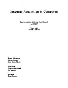
English population as a whole might remain biased toward OV for too long and be unable to reach an average pVO of 0.75 by 1200 A.D. Figure 2 displays the average pVO in the population at 1200 A.D. for six Old English populations whose learners had different amount of degree-1 data available in the input (and therefore in their intake when the degree-0 filter is dropped). The modeling results suggest that having even 4% degree-1 data available in the input is enough to prevent the simulated Old English population from having an average pVO of 0.75 by 1200 A.D. Now, abstracting away from the issue of ambiguity, how much degree-1 data were in the input to Old English learners? Estimates from samples of modern English children’s input (see Appendix C for details) suggest that at least 15%–16% of it is degree-1 data. If we assume that the amount of degree-1 child-directed data is approximately the same no matter what period they live in (and we are currently unaware of studies that suggest otherwise), then we estimate that Old English children also heard degree-1 data about 15%–16% of the time in the input. The modeling results show that allowing in 16% degree-1 data causes the simulated Old Eng-
FIGURE 2 Average probability of accessing VO order at 1200 A.D. for populations with differing amounts of degree-1 data available during acquisition, as compared to the estimated average from historical corpora. Confidence intervals of 95% are shown as well.
INPUT FILTERING IN SYNTACTIC ACQUISITION
61
TABLE 5 OV Advantage in the Input at 1000 A.D Without Unambiguous and Degree-0 Data Filters
D0 Clauses D1 Clauses
Total Clauses
OV Data Intake
VO Data Intake
OV Advantagea
9,805 7,559
2,537 4,650
3,889 2,610
(2537–3889)/9805 = –13.8% (1,759–992)/7,559 = 10.1%
Note. OV = object–verb; VO = verb–object. aWe derive the advantage for the OV order by subtracting the quantity of VO data in the intake from the quantity of OV data in the intake, and then dividing by the total number of clauses. Note that a negative OV advantage means that the VO order has the advantage in the input.
lish population to be far too slow in shifting to a strongly VO distribution. Unless there is a way for the learner to allow in only a quarter of the degree-1 data available in the input, these modeling results suggest that the degree-0 data filter on the input is also necessary.
Both unambiguous data and degree-0 data filters. One might wonder if dropping both the unambiguous data filter and the degree-0 data filter would allow the population to become strongly VO at the right time. If both these filters are dropped, we get the following OV advantage in the input from the historical corpora data for 1000 A.D. (see Table 5). For the Old English population to remain strongly OV before 1150 A.D., OV order must have the advantage in the input—but it is VO order that has the advantage instead. To drop the VO advantage down to zero (so OV order has at least a fighting chance with learners at 1000 A.D.), 56% of in input would have to consist of degree-1 data. Given that our estimate for the amount of degree-1 data is 16%, less than a third this amount, it seems that we cannot drop both the unambiguous data filter and the degree-0 data filter, because the Old English population is still driven to become strongly VO too soon. The claim that both input filters are necessary is therefore strengthened.
DISCUSSION We provide empirical support for proposals that claim that early syntactic acquisition proceeds by filtering the input available to learners down to the degree-0 unambiguous data. We construct an existence proof by showing that a filtered model can handle the particular case of word order change. Two concerns exist regarding the general availability of such data and the complexity of computing this ambiguity. Moving beyond this case and even assuming that unambiguous data are highly informative and crucial for acquisition, such data may be quite difficult for the
62
PEARL AND WEINBERG
learner to find in the observable data given alternative grammatical assumptions— and we have only considered one instance of change.5 If the initial intake is to contain any examples at all, it may well be necessary to allow data that are ambiguous to be considered unambiguous at the initial stage of learning. One way to accomplish this is to restrict the set of parameters relevant for parsing to some initial pool. Thus, the set of parameters that a learner initially uses to discover unambiguous data is a subset of the set of parameters an adult uses when parsing.6 The markedness assumption of Fodor (1998a) might also be used to restrict the initial pool of parameters: default values are assumed for some parameters until the learner is forced to the marked values. For example, in the case discussed in this article, the child might assume that there is no movement as a default assumption (thus allowing unambiguous analysis of simple SVO structures until cases that do not comport with this assumption are discovered in simple data). This hypothesis can then be revised at a later stage. This may, however, have a cost in the form of reanalysis. Suppose that we have two parameters, P1 and P2, and the correct adult value for parameter P1 is P1b. If a parameter P2 is not available to the learner during parsing, suppose that the learner encounters unambiguous data for a value P1a of parameter P1. When P2 becomes available to the learner (perhaps due to the learner’s increased understanding of the simpler parameters of the language, which then allows the learner to become aware of more complex parameters), the learner suddenly discovers that the previous P1a unambiguous data are now ambiguous and that there instead exist unambiguous data for P1b. In this way, parameters that interact (here, P1 and P2) but that are not all in the learner’s parsing pool may force the learner to reanalyze later, when all the interacting parameters become available. This reanalysis, however, seems a reasonable price to pay for the ability to learn something and, in effect, get off the ground. Assuming that parameters are independent structural pieces when parsing is beneficial to ensuring sufficient unambiguous data and efficient computation of ambiguity. With independent parameters, and assuming n parameters with two options each, every sentence has at most 2n possible structural pieces to use during parsing (Fodor, 1998a, 1998b; Sakas & Fodor, 1998); without independent parameters, every sentence has 2n possible structures—because each structure is a combination of n structural pieces. Thus, assuming that parameters are independent is enormously more efficient for parsing a single sentence. Moreover, unambiguous data are then unambiguous relative to a particular parameter—data may be unambiguous for one parameter while being ambiguous for many other parameters. The 5Special thanks to Brian MacWhinney and others at the Psychocomputational Models of Human Language Acquisition workshop in 2005 for pointing this out. 6A candidate set for the initial pool of parameters might be derived from a hierarchy of parameters, along the lines of the one based on cross-linguistic comparison described in Baker (2001, 2005).
INPUT FILTERING IN SYNTACTIC ACQUISITION
63
learner knows if only one of the structural options available for a particular parameter leads to a successful parse, so there is no question which parameter’s probabilistic weighting should be adjusted. In contrast, if parameters are not independent, only data that are unambiguous for all parameters are unambiguous—otherwise, more than one structure of n structural pieces leads to a successful parse. Such data are likely to be extremely sparse, if they exist at all. Turning now to the model’s predictions regarding the frequency of language change: the nature of the input filter may be what differentiates situations of language change from situations of stable variation. If the intake becomes too mixed for the child to converge to the same probabilistic weighting as the adult, then language change will occur. In cases where only one structural option is used in the adult population (as is often the case), the adult probabilistic weighting will be 0.0 or 1.0. Given children’s tendency to generalize to an extreme value from noisy data (Hudson Kam & Newport, 2005), the intake has to be quite mixed to force children away from the adult weighting. In this way, acquisition can tolerate some variation in the input without causing the language to change. In this, our model’s behavior differs notably from that of Briscoe (2000), who observed constant oscillation in the population due to slight variation in the input to learners. Our model differs from his by using only unambiguous data to update the learner’s hypothesis. We also allow the learner’s final probability to be a value other than 0.0 or 1.0. We hypothesize that this is what yields the historically correct behavior. In addition, the model here has more realistic estimates for input quantity, population size, and learner life span.
CONCLUSION We assume that certain types of language change result from a misalignment of the child’s hypothesis and an adult’s analysis of the same data. We then answer questions about language acquisition using models of language change. We show that our input filters on simulated learners during acquisition were crucial to simulation of change at the same rate as the Old English population. Because this language change is thought to be driven by language acquisition, we conclude that children must use these input filters during normal acquisition. We emphasize that, unlike real-world experimentation, our analysis demonstrates that we can restrict the input to the modeled learners and see the results. This is empirical support because the data that compose the intake to individual learners are essential to the trajectory of the language change in the population . It is ideally now clear how models of language change can have implications for language acquisition theory in the general case, and we look forward to using this method to examine other acquisition proposals. Future work will test the necessity
64
PEARL AND WEINBERG
of an unambiguous data filter during learning via simulation in other domains, such as learning phonological stress (Dresher, 1999).
ACKNOWLEDGMENT This work is supported by an NSF Graduate Fellowship. We are immensely grateful to Charles Yang, Garrett Mitchener, LouAnn Gerken, Susan Goldin-Meadow, David Lightfoot, Suzanne Stevenson, William Sakas, Ted Briscoe, Norbert Hornstein, Stephen Crain, Rosalind Thornton, Tony Kroch, Beatrice Santorini, Ann Taylor, Susan Pintzuk, Philip Resnik, Cedric Boeckx, Partha Niyogi, Michelle Hugue, three anonymous reviewers, and the audiences of the Second Workshop on Psychocomputational Models of Human Language Acquisition, ICEHL 13, DIGS VIII, the 28th PLC, the Cognitive Neuroscience of Language Lunch Talks, and the 2003 Maryland Student Conference.
REFERENCES Bailey, C-J. (1973). Variation and linguistic theory. Washington, DC: Center for Applied Linguistics. Baker, M. (2001). The atoms of language: The mind’s hidden rules of grammar. New York: Basic Books. Baker, M. (2005). Mapping the terrain of language learning. Language Learning and Development, 1, 93–129. Bock, J., & Kroch, A. (1989). The isolability of syntactic processing. In G. Carlson & M. Tannenhaus (Eds.), Linguistic structure in language processing (pp. 157–196). Boston: Kluwer. Briscoe, T. (1999). The acquisition of grammar in an evolving population of language agents. Electronic Transactions on Artificial Intelligence, 3, 47–77. Briscoe, T. (2000). An evolutionary approach to (logistic-like) language change. Unpublished manuscript, University of Cambridge, England. Clark, R., & Roberts, I. (1993). A computational model of language learnability and language change. Linguistic Inquiry, 24, 299–345. Cosmides, L., & Tooby, J. (1996). Are humans good intuitive statisticians after all? Rethinking some conclusions from the literature on judgement and uncertainty, Cognition, 58, 1–73. Dresher, E. (1999). Charting the learning path: Cues to parameter setting. Linguistic Inquiry, 30, 27–67. Elman, J. L. (1993). Learning and development in neural networks: The importance of starting small. Cognition, 48, 71–99. Fodor, J. D. (1998a). Parsing to learn. Journal of Psycholinguistic Research, 27(3), 339–374. Fodor, J. D. (1998b). Unambiguous triggers. Linguistic Inquiry, 29, 1–36. Gerken, L. (2006). Decision, decisions: Infant language learning when multiple generalizations are possible. Cognition, 98, B67–B74. Hudson Kam, C. L., & Newport, E. L. (2005). Regularizing unpredictable variation: The roles of adult and child learners in language formation and change. Language Learning and Development, 1, 151–195. Koenigsberger, H. G., & Briggs, A. (1987). Medieval Europe, 400–1500. New York: Longman.
INPUT FILTERING IN SYNTACTIC ACQUISITION
65
Kroch, A., & Taylor, A. (1997). Verb movement in Old and Middle English: Dialect variation and language contact. In A. van Kemenade & N. Vincent (Eds.), Parameters of morphosyntactic change (pp. 297–325). Cambridge, England: Cambridge University Press. Kroch, A., & Taylor, A. (2000). The Penn–Helsinki parsed corpus of Middle English (2nd ed.). Philadelphia: University of Pennsylvania, Department of Linguistics. Lightfoot, D. (1991). How to set parameters. Cambridge, MA: MIT Press. Lightfoot, D. (1999). The development of language: Acquisition, change, and evolution. Oxford, England: Blackwell. MacWhinney, B. (1995). The CHILDES project: Tools for analyzing talk. Mahwah, NJ: Lawrence Erlbaum Associates, Inc. Manning, C., & Schütze, H. (1999). Foundations of statistical natural language processing. Cambridge, MA: MIT Press. Morgan, J. L. (1986). From simple input to complex grammar. Cambridge, MA: MIT Press. Niyogi, P., & Berwick, R. (1995). The logical problem of language change [AI Memo No. 1516]. Cambridge, MA: MIT, Artificial Intelligence Laboratory. Niyogi, P., & Berwick, R. (1996). A language learning model for finite parameter spaces. Cognition, 61, 161–193. Niyogi, P., & Berwick, R. (1997). Evolutionary consequences of language learning. Linguistics and Philosophy, 20, 697–719. Osgood, C., & Sebeok, T. (1954). Psycholinguistics: A survey of theory and research problems. Journal of Abnormal and Social Psychology, 49, 1–203. Pintzuk, S. (2002). Verb–object order in Old English: Variation as grammatical competition. In D. W. Lightfoot (Ed.), Syntactic effects of morphological change (pp. 276–299). Oxford, England: Oxford University Press. Rohde, D., & Plaut, D. (1999). Language acquisition in the absence of explicit negative evidence: How important is starting small? Cognition, 72, 67–109. Sakas, W. G. (2003). A word-order database for testing computational models of language acquisition. In Proceedings of the 41st annual meeting of the Association for Computational Linguistics (pp. 415–422). Sapporo, Japan: ACL. Sakas, W. G., & Fodor, J. D. (1998). Setting the first few syntactic parameters: A computational analysis. In Proceedings of the 20th annual conference of the Cognitive Science Society (pp. 917–922). Mahwah, NJ: Lawrence Erlbaum Associates, Inc. Taylor, A., Warner, A., Pintzuk, S., & Beths, F. (2003). The York–Toronto–Helsinki parsed corpus of Old English. York, England: University of York, Department of Language and Linguistic Science. Tenenbaum, J., & Griffiths, T. (2001). Generalization, similarity, and Bayesian inference. Behavioral and Brain Sciences, 24, 629–640. Weinreich, U., Labov, W., & Herzog, M. (1968). Empirical foundations for a theory of language change. In W. Lehmann and Y. Malkiel (Eds.), Directions for historical linguistics (pp. 97–195). Austin: University of Texas Press. Wexler, K., & Culicover, P. (1980). Formal principles of language acquisition. Cambridge, MA: MIT Press. Yang, C. (2000). Internal and external forces in language change. Language Variation and Change, 12, 231–250. Yang, C. (2003). Knowledge and learning in natural language. Oxford, England: Oxford University Press. Yang, C. (2004). Universal grammar, statistics or both? Trends in Cognitive Science, 8(10), 451–456.
66
PEARL AND WEINBERG
APPENDIX A Bayesian Updating of the Learner’s Current Hypothesis The learner in our model has a single value pVO, which represents the learner’s confidence about encountering a VO order utterance. This value is updated as each piece of data from the intake is encountered by taking the maximum of the a posteriori (MAP) probability of the prior belief pVOprev (Manning & Schütze, 1999). We represent the learner’s hypothesis of the distribution of OV and VO utterances as a binomial distribution centered around pVO. Our learner considers only the current piece of data, so the length of the input sequence s for the Bayesian updating is 1. We assign an OV utterance value 0 in the binomial distribution and a VO order utterance value 1. The learner’s prior belief pVOprev of the learner is the expected probability that a VO utterance will be encountered during the period of fluctuation. Our initial pVO of 0.5 means that one expects an OV or VO utterance with equal probability. To update pVO, we take the MAP probability of pVO, given the current piece of input: pVO = max(Prob(pVOprev | s)) (via Bayes’ rules) =
max( Prob( s| p VOprev ) * Prob(p VOprev ) Prob( s)
For ease of legibility, p = pVOprev below. If s = VO utterance Prob(s | p) = p n Prob( p) = * p r *(1 − p) n − r r for each r = 0 to n in the binomial distribution. To update, we take the MAP probability by setting the derivative with respect to p (d/dp) = 0 and then solve for p. n r p * * p * p(1 − p) n − r d r Prob( s) dp
=0
INPUT FILTERING IN SYNTACTIC ACQUISITION
n p * * p r *(1 − p) n − r r d dp Prob( s)
67
=0
(Prob(s) is a constant dp) p = (r+1)/(n+1) r = previous expected number of unambiguous VO utterances to be seen out of n unambiguous utterances during the fluctuation period. If previous probability was pVOprev, then previous expected number out of n was pVOprev * n. Updated probability pVO = (pVOprev * n + 1)/(n + 1). If s = OV utterance, the same process can be followed to give pVO = (pVOprev * n)/ (n + 1). Thus, pVO depends on the prior probability of a VO utterance (pVOprev) and the number of unambiguous utterances expected during the fluctuation period (n). Unfortunately, this update process does not converge to 1 or 0 with n = 2,000 unambiguous utterances, even if all unambiguous data are of one value (if all OV, the final p is 0.194—not 0.0; if all VO, the final p is 0.816—not 1.0). We modified the update method to allow the final pVO to be closer to the endpoint value (either 0.0 or 1.0) for each case. We do this by substituting a confidence value c for 1 in the update function: VO data: pVO = ((pVOprev * n + c)/(n + c) OV data: pVO = ((pVOprev * n)/(n + c) The value c ranges linearly between 0 and a max value m, depending on what pVOprev is VO data: c = pVOprev * m OV data: c = (1 – pVOprev) * m m ranges between 3 and 5. The m for a particular mixture of degree-0 and degree-1 data is determined by seeing which m value allows the simulated Old English population to reach the “checkpoint” average pVO value of .31 between 1000 A.D. and 1150 A.D. With the new update functions, unambiguous data for one value the entire time will cause the final pVO to be much closer to the endpoint. Seeing 2,000 OV utter-
68
PEARL AND WEINBERG
ances leaves pVO between .007 and .048 (depending on m), and seeing 2,000 VO utterances leaves pVO between .952 and .993 (depending on m).
APPENDIX B Estimating pVO Both the degree-0 and degree-1 unambiguous data distributions are likely to be distorted from the underlying unambiguous data distribution produced by pVO because the degree-0 and degree-1 clauses have ambiguous data. The underlying distribution in a speaker’s mind, however, has no ambiguous data—every clause is generated with OV or VO order. As we saw in Table 2, the degree-0 clauses have more ambiguous data than the degree-1 clauses; therefore, we make the assumption that the degree-0 distribution is more distorted than the degree-1 distribution. We then use the difference in distortion between the degree-0 and degree-1 unambiguous data distributions to estimate the difference in distortion between the degree-1 distribution and the underlying unambiguous data distribution in a speaker’s mind. In this way, we estimate the underlying unambiguous data distribution (produced by pVO) for an average Old English speaker at certain points in time. We demonstrate how we estimate pVO at 1000 A.D. (see Table B1).
Observation 1. The degree-0 data have many more ambiguous clauses than do the degree-1 data. This is seen by comparing the percentage of ambiguous data (see Table B2). Observation 2. The degree-1 distribution is always more “biased” than the degree-0 distribution toward one of the endpoints—completely OV (pVO = 0.0) or VO (pVO = 1.0). If the degree-0 distribution favors OV order, the degree-1 distribution favors it even more; if the degree-0 distribution favors VO order, the degree-1 distribution favors it even more. TABLE B1 Data Counts From Historical Corpora Degree-0 Data
1000 A.D. 1000–1150 A.D. 1200 A.D.
Ambig
Unambig
7,480 5,000 912
2,325 1,214 370
Degree-1 Data %
Ambiga 76 80 71
Ambig
Unambig
% Amba
2,132 902 225
5,427 2,734 2,011
28 25 10
aThe percentage of ambiguous clauses is calculated by dividing the number of ambiguous clauses by the total number of ambiguous and unambiguous clauses.
69
INPUT FILTERING IN SYNTACTIC ACQUISITION
TABLE B2 Unambiguous Data Counts From Historical Corpora Unambiguous Degree-0
1000 A.D. 1000–1,150 A.D. 1200 A.D.
OV
VO
% VOa
1,389 624 180
936 590 190
40 49 51
Unambiguous Degree-1 OV
VO
3,844 1,759 551
1,583 975 1,460
% VOa 29 36 73
Note. OV = object–verb; VO = verb–object. aThe percentage of VO is calculated by dividing the quantity of unambiguous VO data by the total quantity of unambiguous data.
Assumption. Both the degree-0 and degree-1 distribution of OV and VO unambiguous data are skewed from the underlying distribution of unambiguous data in the average Old English speaker’s mind. The degree-0 distribution is skewed more than the degree-1 distribution. Thus, the underlying distribution of unambiguous data should be even more “biased” toward completely OV (pVO = 0.0) or VO (pVO = 1.0) than the degree-1 distribution is. We now use skew in the degree-0 and degree-1 distribution to estimate the skew between the degree-1 and the underlying distribution. We use the data from 1000 A.D. as an example. Degree-0 total clauses: 9,805 (= ambiguous + unambiguous = 7,480 + 2,325) Degree-0 unambiguous OV: 1389 Degree-0 unambiguous VO: 936 Step 1. Normalize degree-1 quantities to match degree-0 quantities. If there had been the same number of degree-1 clauses as degree-0 clauses, how many would have been unambiguous OV data, and how many would have been unambiguous VO data? Degree-1 total: 7,559 (= Ambiguous + Unambiguous = 2,132 + 5,427) Normalize → degree-1 total = 7,559 * 9,805/7,559 = 9,805 degree-1 unambiguous OV: 3,844 Normalize → degree-1 unambiguous OV = 3,844 * 9,805/7,559 = 4,986 Degree-1 unambiguous VO: 1,583 Normalize → degree-1 unambiguous VO = 1,583 * 9,805/7,559 = 2,053 Degree-1 ambiguous = degree-1 total – (OV + VO) = 9,805 – (4,986 + 2,053) = 2,766 (see Table B3). Step 2. Compare degree-0 and normalized degree-1 quantities to determine how much additional loss happened in the degree-0 clauses for whatever reason (see Table B4).
70
PEARL AND WEINBERG
TABLE B3 Normalized Degree-1 Distribution 1000 A.D. Normalized Degree-1 Note.
Clauses
Ambiguous
Unambiguous OV
Unambiguous VO
9,805
2,766
4,986
2,053
OV = object–verb; VO = verb–object.
TABLE B4 Additional Loss Calculations 1000 A.D. Degree-0 Normalized Degree-1 Number lost between D1 and D0 Note.
Unambiguous OV
Unambiguous VO
1,389 4,986 4,986–1,389 = 3,597
936 2,053 2,053–936 = 1,117
OV = object–verb; VO = verb–object.
Step 3. Calculate “loss ratio.” For each unambiguous OV clause “lost” (because it became ambiguous), how many unambiguous VO clauses were “lost”? Loss ratio = (# unamb OV lost)/(# unamb VO lost) = 3,597/1,117 = 3.22 Thus, the unambiguous OV data are about 3 times as likely to become ambiguous as the unambiguous VO data are (again, for whatever reason).
Step 4. Describe what is known about the degree-1 distribution and the underlying distribution. The degree-1 distribution is a skewed version of the underlying distribution in the average Old English speaker’s mind. In the underlying distribution, all data are unambiguous because they are generated with either OV order or VO order (see Table B5). i. x = # of ambiguous data in normalized degree-1 distribution that began as OV ii. y = # of ambiguous data in normalized degree-1 distribution that began as VO iii. # of ambiguous data in normalized degree-1 distribution = 2,766
Step 5. Create equations to solve for unknown variables x and y. i. x + y = 2,766 (based on 4.iii above) ii. % OV unambiguous data lost from underlying distribution to D1 distribution = x/(4,986 + x) iii. % VO unambiguous data lost from underlying distribution to D1 distribution = y/(2,053 + y)
71
INPUT FILTERING IN SYNTACTIC ACQUISITION
TABLE B5 Comparing Degree-1 Distribution to the Underlying Distribution
1000 A.D. Normalized Degree-1 Underlying Note.
Total
Ambiguous
Unambiguous OV
Unambiguous VO
9,805 4,986 + x + 2,053 + y
2,766 0
4,986 4,986 + x
2,053 2,053 + y
OV = object–verb; VO = verb–object. TABLE B6 Data From Historical Corpora and Calculated pVO Degree-0 Clauses
1000 A.D. 1000–1150 A.D. 1200 A.D. Note.
Degree-1 Clauses
Underlying
Total
OV Unambig
VO Unambig
Total
OV Unambig
VO Unambig
pVO
9,805 6,214 1,282
1,389 624 180
936 590 190
7,559 3,636 2,236
3,844 1,759 551
1,583 975 1,460
0.233 0.310 0.747
OV = object–verb; VO = verb–object; Unambig = unambiguous.
If we assume that the loss ratio does not change (the unambiguous OV data are still about 3 times as likely as the unambiguous VO data to become ambiguous), we can get the following: iv. (OV % loss) = (loss ratio) * (VO % loss) x/(4,986 + x) = 3.22 * (y/(2,053 + y)) Using i and iv together, we solve to get x = 2,536 and y = 2,766 – 2,536 = 230
Step 6. Classify ambiguous data, and calculate underlying distribution pvo. Unambiguous OV data in underlying distribution = 4,986 + 2,536 = 7,522 Unambiguous VO data in underlying distribution = 2,053 + 230 = 2,283 Underlying pVO at 1000 A.D. = 2,283/(7,522 + 2,283) = .233 The remaining two pVO values can be calculated the same way (see Table B6).
APPENDIX C Estimating Degree-1 Percentage in the Input To get a sense of how much of an average child’s input consists of degree-1 clauses, we sampled a small portion of the CHILDES database (MacWhinney, 1995) and some young children’s stories (some of which can be found at http:// www.magickeys.com/books/index.html). We used CHILDES because it is re-
72
PEARL AND WEINBERG
corded speech to children and young children’s stories because it is language designed to be read to children (see Table C1). We take the average of these two sources to get approximately 16% degree-1 data available in children’s input. This is similar to the 15% degree-1 data estimate from Sakas (2003), who examined several thousand sentences from the CHILDES database.
TABLE C1 Data Gathered From Speech Directed to Young Children Total Utterances
Total Clausesa
A subsection of CHILDES 4,068 2,760 Sample D0 Utterances “What’s that?” “I don’t know.” “There’s a table.” “Can you climb the ladder?” “Shall we stack these?” “That’s right.” Young Children’s Stories 4,031 3,778 Sample D0 Utterances “Ollie is an eel.” “She giggled.” “ … but he climbs the tree!” “This box is too wide.” “ … to gather their nectar.”b, “This is the number six.”
Total D0
2,516
Total D1
244 Sample D1 Utterances
% D1
8.8
“I think it’s time … ” “Look what happened!” “I think there may be one missing.” “Show me how you play with that.” “See if you can get it.” “That’s what he says.” 2,955
927 Sample D1 Utterances
23.9
“ … that even though he wishes hard, … ” “ … that only special birds can do.” “ … that can repeat words people say.” “ … when the sun shines.” “ … that goes NEIGH … NEIGH … ” “ … know what it is?”
aThe number of clauses is much less than the number of utterances because many of these utterances include “Huh?” and exclamations such as “A ladder!” in the case of the spoken CHILDES corpus. For the young children’s stories, there are often “sentences” such as “Phew!” and “Red and yellow and green,” which were excluded under total clauses. bWe note that clauses with infinitives, such as “ … to gather their nectar,” are included under degree-0 data, based on Lightfoot’s (1991) definition of clause–union structures as degree-0. If this were not the case, the percentage of degree-1 clauses would be higher than what we calculated here—thus, this is a lower bound on the amount of degree-1 data available in the input.