Insight into Binary Star Formation via Modelling Visual Binaries Datasets © Oleg Malkov © Dmitry Chulkov © Dana Kovaleva © Alexey Sytov © Alexander Tutukov © Lev Yungelson Institute of Astronomy, Russian Academy of Sciences, Moscow, Russia
[email protected] [email protected] [email protected] [email protected] [email protected] [email protected] © Yikdem Gebrehiwot Entoto Observatory and Research Center, Addis Ababa, Ethiopia Mekelle University, College of Natural and Computational Sciences, Mekelle, Ethiopia
[email protected] © Nikolay Skvortsov Institute of Informatics Problems, Federal Research Center "Computer Science and Control", Russian Academy of Sciences, Moscow, Russia
[email protected] © Solomon Belay Tessema Ethiopian Space Science and Technology Institute, Entoto Observatory and Research Center Astronomy and Astrophysics, Addis Ababa, Ethiopia tessemabelay@gmail com Abstract. We describe the project aimed at finding initial distributions of binary stars over masses of components, mass ratios of them, semi-major axes and eccentricities of orbit, and also pairing scenarios by means of Monte-Carlo modeling of the sample of about 1000 visual binaries of luminosity class V with Gaia DR1 TGAS trigonometric parallax larger than 2 mas, limited by 2 ≤ 𝜌𝜌 ≤ 200 arcsec, 𝑉𝑉1 ≤ 9.5𝑚𝑚 , 𝑉𝑉2 ≤ 11.5𝑚𝑚 , ∆𝑉𝑉 ≤ 4𝑚𝑚 , which can be considered as free of observational incompletness effects. We present some preliminary results which allow already to reject initial distributions of binaries over semi-major axes of the orbits more steep than ∝ 𝑎𝑎−1.5 . Keywords: binary stars, stellar formation, modeling which, combined, we will call “the birth function” (henceforth, BF). Most important, BF is, first, a benchmark for the theories of star formation and, second, the base for the estimates of the number of objects in the models of different stellar populations and model rates of various events, e. g., supernovae explosions etc. In the present study, we assume that BF is defined by three fundamental functions describing distribution of stars over initial mass of primary component 𝑀𝑀1 , mass ratio of components 𝑞𝑞, and semi-major axes of orbits 𝑎𝑎 [25]. It was suggested by Vereshchagin et al. (1988) [35] that BF for visual binaries has the form
1 Introduction Majority of stars accessible for detailed observational study appear to be binary ones. Interaction between binary star components in the course of their evolution results in a rich variety of astrophysical phenomena and objects. Study of the structure and evolution of binary stars is one of the most actively developing fields of the modern astrophysics. Among fundamental problems aimed by these studies is the one of initial distributions of binary stars over their main parameters: • mass of the primary component 𝑀𝑀1 , • mass ratio of components 𝑞𝑞 = 𝑀𝑀2 ⁄𝑀𝑀1 , • and semi-major axis 𝑎𝑎 of component orbits,
d3 𝑁𝑁 ∝ 𝑀𝑀1−2.5 d 𝑀𝑀1 ∙ d log 𝑎𝑎 ∙ 𝑞𝑞 −2.5 d𝑞𝑞 𝑦𝑦𝑦𝑦𝑦𝑦𝑦𝑦 −1
(1)
where M1 and 𝑎𝑎 are expressed in solar units. As a “minor” characteristics, we consider eccentricity of orbits 𝑒𝑒. The aim of the current paper is presentation of preliminary results of the assessment of BF by means of
Proceedings of the XX International Conference “Data Analytics and Management in Data Intensive Domains” (DAMDID/RCDL’2018), Moscow, Russia, October 9-12, 2018
98
comparison of results of Monte-Carlo model of the local population of field visual binaries with their observed sample. We probe, for a given type of stars, whether the synthetic dataset differs significantly due to the change of initial fundamental distributions, and how the change of every distribution affects it. For this purpose, we compare synthetic populations for different pairing functions and particular sets of fundamental functions. We attempt to find whether certain initial distributions or combinations of initial distributions result in synthetic datasets incompatible with observational data at certain significance level and, on the contrary, whether certain initial distributions or combinations of initial distributions provide synthetic dataset best compatible with observational data, hopefully, at certain significance level. The model also accounts for star formation rate, stellar evolution and takes into account observational selection effects. The model is compared to the dataset compiled as described by Kovaleva et al [18] with addition of the data on parallaxes from Gaia DR1 TGAS [9]. Besides, our model allows to obtain estimates for the fraction of binary stars that remains unseen for different reasons and is observed as single objects and to investigate how these fractions depend on the initial distributions of parameters. Such estimates are important, for instance, as an approach toward recovering actual multiplicity fraction, mass hidden in binaries, as well as toward models of different stellar populations. The model and observational data are described in chapters 2 and 3, respectively. Some considerations on the choice of theoretical models are described in chanter 4. Results and conclusions are presented in chapter5. In chapter 6 we outline the plans of future studies.
the short summary of the used pairing functions. Masses of the of components or total masses of the binaries were drawn randomly from Salpeter [32] or Kroupa [21] initial mass functions (IMF), separation 𝑎𝑎 was drawn from one of the following distributions: ∝ 𝑎𝑎−1 , ∝ 𝑎𝑎 −1.5 , ∝ 𝑎𝑎−2 , and eccentricity 𝑒𝑒 was distributed assuming following options: (i) all orbits are circular, (ii) eccentricities obey thermal distribution 𝑓𝑓𝑒𝑒 (𝑒𝑒) = 2𝑒𝑒, and (iii) equiprobable distribution 𝑓𝑓𝑒𝑒 (𝑒𝑒) = 1. We adopt random orbit orientation. Mass ratio 𝑞𝑞, when needed, is randomly drawn from ∝ 𝑞𝑞 𝛽𝛽 distribution, where 𝛽𝛽 is adopted to be −0.5, 0 or −0.5. The lower limit for 𝑞𝑞 is determined by mass limits [0.08 ⋯ 100] 𝑀𝑀⊙ . Certain pairing functions, such as RP, PCRP, PSCP and TPP, do not allow independent random distribution of mass ratios, it is calculated from masses of components. Table 2 contains short summary on initial distributions used in the modelling. Some cells are empty because the pre-planned distributions are not implemented as yet. The total number of possible combinations of initial distributions considered as yet is 144, equal to the number of possible combinations of 𝑠𝑠, 𝑚𝑚, 𝑞𝑞, 𝑎𝑎, 𝑒𝑒 in Table 2 and regarding that 𝑠𝑠0 and 𝑠𝑠5 scenarios do not imply independent initial distribution over 𝑞𝑞 (see Table 1). Any combination of distributions listed in Table 2 can be conveniently referred, for instance, as “s2m0q5a1e0”. To account for star formation rate we adopt SFR(t) = 15 e−t/7 , where the time t is expressed in Gyr (Yu & Jeffery 2010 [36]). Disc age is assumed to be equal to 14 Gyr. Currently, we consider the following stellar evolutionary stages: MS-star, red giant, white dwarf, neutron star, black hole. The objects in the two latter stages do not produce visual binaries (though they contribute to the statistics of pairs, observed as single stars, see Section 5.2 below). We do not consider brown dwarfs and pre-MS stars here, as they are extremely rarely observed among visual binaries and their multiplicity rate is substantially lower than for more massive stars (Allers 2012) [1]. As we deal with wide pairs only, we assume the components to evolve independently. To calculate evolution of stars and their observational properties we used analytical expressions derived by Hurley et al [15] and assumed solar metallicity for all generated stars. To normalize the number of simulated objects, we use estimates of stellar density in the solar neighborhood, based on recent Gaia results [4]. The data for A0V-K4V stars presented by Bovy (2017) [4] give 0.01033 stars per pc3. This means that in the 500 pc sphere we generate about 43300 pairs of stars. For the generated objects, we determine observational parameters, in particular, the brightness of components, their evolutionary stage and projected separation. Then we apply a filter to select a sample of stars, which can be compared with observational data (see the next section).
2 The model Visual binaries are observed, mostly, in the immediate solar vicinity. Therefore, we consider them to be distributed up to the distance of 500 pc in radial direction and according to a barometric function along z. The scale height z for the stars of different spectral types and, respectively, masses was studied, e. g., in [3,10,12,20,31]. Synthesizing results of these studies, we assume |z| = 340 pc for low-mass (≤ 1 𝑀𝑀⊙ ) stars, 50 pc for high-mass (≥ 10 𝑀𝑀⊙ ) stars, and linear |z| − log 𝑀𝑀 relation for intermediate masses. For such a small volume we can neglect the radial gradient (Huang et al. 2015) [14]. We also ignore interstellar extinction. To simulate stellar pairs we use different pairing functions (scenarios), mostly taken from Kouwenhowen's list [16]. It includes random pairing and other scenarios, where two of the four parameters (primary mass, secondary mass, total mass of the system, mass ratio) are randomized, and other are calculated. Table 1 contains
99
Table 1 Summary of considered pairing functions (scenarios) Abbreviation
Full name
Scheme
RP
Random Pairing
PCRP
Primary Constrained Random Pairing
PCP
Primary Constrained Pairing
SCP
Split-Core Pairing
PSCP
Primary Split-Core Pairing
TPP
Total Primary Pairing
rand(M1 , M2 , [M𝑚𝑚𝑚𝑚𝑚𝑚 ⋯ M𝑚𝑚𝑚𝑚𝑚𝑚 ]); sort(M1 , M2 ); calc(𝑞𝑞).
rand(M1 , [M𝑚𝑚𝑚𝑚𝑚𝑚 ⋯ M𝑚𝑚𝑚𝑚𝑚𝑚 ]); rand(M2 , [M𝑚𝑚𝑚𝑚𝑚𝑚 ⋯ M𝑚𝑚𝑚𝑚𝑚𝑚 ], M1 = 𝑐𝑐𝑐𝑐𝑐𝑐𝑐𝑐𝑐𝑐 until M2 < M1 ); calc(𝑞𝑞). rand(M1 , 𝑞𝑞); calc(M2 ).
rand(M𝑡𝑡𝑡𝑡𝑡𝑡 , [2M𝑚𝑚𝑚𝑚𝑚𝑚 ⋯ 2M𝑚𝑚𝑚𝑚𝑚𝑚 ]); rand(𝑞𝑞); calc(M1 , M2 ).
rand(M𝑡𝑡𝑡𝑡𝑡𝑡 , [2M𝑚𝑚𝑚𝑚𝑚𝑚 ⋯ 2M𝑚𝑚𝑚𝑚𝑚𝑚 ]); rand(M1 , [0.5(M1 +M2 ) ⋯ M𝑚𝑚𝑚𝑚𝑚𝑚 ], until M1 < M𝑡𝑡𝑡𝑡𝑡𝑡 ); calc(M2 ); calc(q). rand(M𝑡𝑡𝑡𝑡𝑡𝑡 , [2M𝑚𝑚𝑚𝑚𝑚𝑚 ⋯ 2M𝑚𝑚𝑚𝑚𝑚𝑚 ]); rand(M1 , [M𝑚𝑚𝑚𝑚𝑚𝑚 ⋯ M𝑚𝑚𝑚𝑚𝑚𝑚 ], until M1 < M𝑡𝑡𝑡𝑡𝑡𝑡 ); calc(M2 ); sort(M1 , M2 ); calc(q).
Note: M𝑡𝑡𝑡𝑡𝑡𝑡 , M1 , M2 – total mass of the binary, primary mass and secondary mass, respectively; M𝑚𝑚𝑚𝑚𝑚𝑚 , M𝑚𝑚𝑚𝑚𝑚𝑚 – lower (0.08 𝑀𝑀⊙ ) and upper (100 𝑀𝑀⊙ ) limits set for masses; 𝑞𝑞 = 𝑀𝑀2 /𝑀𝑀1 – mass ratio. The meaning of abbreviations is the following: “rand” – randomizing, “calc” – calculation, “sort” – sorting. Table 2 Summary of applied initial distributions sN
Scenario (𝑠𝑠)
mN
0
RP
0 1
2
PCP
3
SCP
IMF (𝑚𝑚) Salpeter
qN 0
Kroupa
TPP
flat, 𝑓𝑓 = 1
aN
Semi-major axis (𝑎𝑎)
eN
0
power, 𝑓𝑓~𝑎𝑎−1
0
power, 𝑓𝑓~𝑎𝑎−2
2
1 2
4 5
Mass ratio (𝑞𝑞)
5
power, 𝑓𝑓~𝑎𝑎
−1.5
1
Eccentricity (𝑒𝑒) thermal, 𝑓𝑓 = 2𝑒𝑒 delta, 𝑓𝑓 = 𝛿𝛿(0) flat, 𝑓𝑓 = 1
power, 𝑓𝑓~𝑞𝑞 −0.5 power, 𝑓𝑓~𝑞𝑞 0.5
incompleteness in the space of observational parameters. The procedure of dataset compilation and analysis described in details in [17,18] was improved due to use of new trigonometric parallaxes from TGAS DR1 Gaia [9] that allowed to re-obtain constraints to avoid regions of observational incompleteness. Out of simulated objects we select pairs, satisfying the same observational constraints, as the refined observational set does, namely: projected separation 2 < 𝜌𝜌 < 200 arcsec, primary component visual magnitude 𝑉𝑉1 < 9.5𝑚𝑚 , secondary component visual magnitude 𝑉𝑉2 < 11.5𝑚𝑚 , magnitude difference Δ𝑉𝑉 ≡ |𝑉𝑉2 − 𝑉𝑉1 | ≤ 4𝑚𝑚 (henceforth, “synthetic dataset”). For the purposes of
3 Observational data for comparison To compare our simulations with observational data, we use the most comprehensive list of visual binaries WCT [17], compiled on the base of the largest original catalogues WDS [24], CCDM [5] and TDSC [8]. These data were refined or corrected for mistaken data, optical pairs, effects of higher degrees of multiplicity, sorted by luminosity class (primarily, to select pairs with both components on the main-sequence), and appended by parallaxes. A refined dataset for comparison was selected from the data, so as to avoid regions of observational
100
correct comparison, we also limit refined set of observational data by 500~pc distance.
As for the eccentricity distribution, from physical point of view, one usually prefers in theoretical simulations the “thermal” law $𝑓𝑓(𝑒𝑒) ∼ 2𝑒𝑒 (Ambartsumian 1937) [2], though in observational datasets one finds, e. g., that the eccentricity distribution of wide binaries contains more orbits with 𝑒𝑒 < 0.2 and less orbits with 𝑒𝑒 > 0.8 (Tokovinin & Kiyaeva 2016 [34]) or a flat distribution in the 𝑒𝑒 = [0.0 ⋯ 0.6] range and declining one for larger 𝑒𝑒 [30]. Having in mind the difficulties hampering determination of eccentricities from observations and numerous selection effects, we probe three quite different model distributions: “thermal”, flat, and single valued with 𝑒𝑒 = 0 for all stars. The very selection of fundamental parameters for initial distribution is arguable. For instance, primary and secondary masses were considered as fundamental parameters for MS binaries by Malkov [23] and pre-MS binaries by Malkov and Zinnecker [22], while Goodwin [11] has argued that system mass is the more fundamental physical parameter to use. We do not reject possibility to choose and investigate other parameters as fundamental ones in the course of further work.
We construct distributions of synthetic datasets over the following parameters: primary and secondary magnitude, magnitude difference, projected separation, parallax. Then we compare the synthetic distributions with refined observational ones using 𝜒𝜒 2 two-sample test. We deem, the better result of comparison, the closer our assumptions on pairing scenarios, initial distributions of masses, mass ratio, separation and eccentricity are to reality. The refined set of observational data contains 𝑁𝑁 = 1089 stars. To compare them properly with results of our simulations we need to use histograms with 𝑛𝑛 = 5 log 𝑁𝑁 bins [33], i. e., 15 ones.
4 Some reflections concerning selection of models In the selection of trial initial distributions for the model we adopted the following approach: we started with well established or widely used in the literature functions for 𝑓𝑓(𝑀𝑀), 𝑓𝑓(𝑎𝑎), 𝑓𝑓(𝑒𝑒) and then stepped aside from them to test, whether the algorithm would be able to feel difference at all. We preferred simple analytical expressions, supposing we would pass to more complicated ones later if we find it necessary. Thus, we use traditional Salpeter's IMF [32] along with the much more recent and generally accepted Kroupa's one [21]. In spite of the statement by Duchêne and Kraus [7] that no observed dataset agrees with random pairing scenario, we use the latter among other ones.
5 Results and discussion 5.1 Star formation function Comparison of our simulations with observational data allows us to make the following preliminary conclusions on initial distributions. Even before application of statistical tests, we should meet a strong and evidently important criterion of validity of the tested combination of initial distributions, namely the agreement between the number of binaries in the simulated datasets and the observed number of visual pairs. This number depends on initial distributions of fundamental variables and changes between 0 and about 15000; an exception is distribution over 𝑒𝑒 which affects the volume of simulated datasets only mildly. Thus, if our accepted normalization [4], along with other used assumptions regarding spatial distribution of visual binaries in solar vicinity is valid, we can exclude certain combinations of initial distributions, based purely on the number of binaries in synthetic dataset. However, our present observational dataset volume (1089 pairs) is limited to binaries having MK spectral classification. Thus, we are careful and do not rely exclusively on this criterion because we allow certain freedom due to simplifications and possible incomplete account of selection effects while constructing the refined observational dataset, as well as to vagueness of theoretical notions on solar vicinity population. This is why we do take into account both number and two sample 𝜒𝜒 2 criteria. Nevertheless, one can definitely reject those combinations of initial distributions that lead to the number of binary stars in a synthetic observational dataset significantly less than 1000 (taking present dataset volume 𝑁𝑁𝑜𝑜𝑜𝑜𝑜𝑜 − �𝑁𝑁𝑜𝑜𝑜𝑜𝑜𝑜 ≈ 1056 as lower limit).
On the other hand, for semi-major axis distribution we applied as yet only commonly used power law parametrization, with the particular case of a log-log flat distribution known as “Öpik’s law” [26]. Validity of 𝑓𝑓𝑎𝑎 ∝ 𝑎𝑎−1 law up to 𝑎𝑎 ≈ 4600 AU, which is close to 𝑎𝑎𝑚𝑚𝑚𝑚𝑚𝑚 of our refined sample of visual binaries, was confirmed by Popova et al [27] and Vereshchagin et al [35] who analyzed the data in the amended 7th Catalog of Spectroscopic Binaries [19] and IDS, respectively. Poveda et al [28], found that Öpik's distribution matches with high degree of confidence binaries with 𝑎𝑎 ≲ 3500 AU (but we note, that selection effects which hamper discovery of the widest systems were not considered, contrary to the abovementioned studies). We also stress, after Heacox [13], that Gaussian distribution of separations encountered in the literature (e. g., Duquennoy & Mayor 1991 [6], Raghavan et al 2010 [30] is an artefact of data representation. Like Poveda et al [28], we reject Gaussian distribution of stellar separations, since it is hard to envision currently a starformation process leading to such a distribution.
101
Figure 1 represents how the resulting 𝜒𝜒 2 statistics are distributed versus number of pairs in the synthetic datasets. The results do not allow us to select “the best” initial distributions over every parameter, but rather to prefer some combinations of initial distributions to others. One may see that no combination leading to acceptable number of pairs in synthetic dataset would give acceptable distribution over angular distances between components, while magnitude difference and, in some cases, distribution over primary magnitudes, are reproduced better for the same initial conditions. Below there are some figures providing examples of how the same distribution over certain parameter, in different combinations with other initial distributions, leads to better or worse agreement with the observational dataset. Figure 2 represents an example of how different combinations of initial distributions change resulting synthetic datasets and their agreement with observational one. Four figures demonstrate, in turn, which values of 𝑁𝑁𝑠𝑠𝑠𝑠𝑠𝑠𝑠𝑠ℎ , 𝜒𝜒 2 correspond to different initial scenarios (𝑠𝑠0, 𝑠𝑠2, 𝑠𝑠4, 𝑠𝑠5, see Table 1, Table 2), IMFs (𝑚𝑚0, 𝑚𝑚1), mass ratio initial distribution (𝑞𝑞0, 𝑞𝑞4, 𝑞𝑞5, applicable solely for the 𝑠𝑠2, 𝑠𝑠3 scenarios), and distribution over semi-major axes 𝑎𝑎0, 𝑎𝑎1, 𝑎𝑎2. Scenarios 𝑠𝑠0 and 𝑠𝑠5 do not involve independent distribution over 𝑞𝑞; it is generated as an outcome of the pairing function and IMF, this is why the 𝑞𝑞-panel contains less dots than the other ones.
Figure 1 Distribution of resulting 𝜒𝜒 2 statistics over number of pairs in the synthetic dataset. Every set of initial distributions of the 144 processed ones results in 4 dots of different colour in this plot. The dashed line marks 5% confidence level of the null-hypothesis (the dots over it correspond to the sets of initial distributions that are rejected at the level of 95%, based on the used observational sample).
Figure 2 Distribution of resulting 𝜒𝜒 2 statistics for magnitude difference Δ𝑉𝑉 vs. number of pairs in the synthetic datasets, depending on various initial distributions, from top to bottom: pairing scenarios (see Tables 1, Table 2), IMFs, distributions over mass ratio (applicable solely for scenarios 𝑠𝑠2, 𝑠𝑠3), and semi-major axes.
102
Figure 3 shows how the distribution over observational parameter magnitude difference changes with the change of one initial distribution (pairing scenarios, IMF, distribution over semi-major axes). The distribution over Δ𝑉𝑉 for the observational dataset serves as a benchmark. Based on combination of the two (number and statistical) criteria, we may (very preliminary) state the following. For the considered observational dataset, RP and TPP pairing scenarios, 𝑠𝑠0 and 𝑠𝑠5 (see Table 1, Table 2), respectively, produce a group of results that seems acceptable in respect of the number of “observed” binaries in the synthetic dataset and, simultaneously, leads to acceptable 𝜒𝜒 2 values at least for two observable distributions (𝑉𝑉1 and Δ𝑉𝑉).
None of the probed combinations of initial distributions can reproduce observational distribution over angular distance between components adequately (see Figure 1). The cause may lay either with selection effects, that still remain unaccounted for (and then the reconsideration of observational sample is necessary), or in need of other initial distributions. Kroupa and Salpeter IMF's lead to different number of pairs in the synthetic dataset, however, neither this difference nor 𝜒𝜒 2 statistics allows definite choice between them. Kroupa IMF looks slightly more promising, than Salpeter one, however, more accurate conclusion should be postponed, as these two IMF differ actually only in the low-mass region, and the majority of visual binaries in our observational dataset presumably have masses around 1 to 3 𝑀𝑀⊙ . The comparison in lowmass region is needed here.
Also, we can not make definite conclusion on the mass ratio 𝑞𝑞 distribution. The 𝑞𝑞-distributions that we have analyzed in the present study show significant difference only in the low-𝑞𝑞 region (below 𝑞𝑞 < 0.5). In the compilative sample of visual binaries used to construct our benchmark dataset, however, binaries with large magnitude differences (and, thus, low 𝑞𝑞) are severely underrepresented. This is why we limit refined observational sample so that pairs with low 𝑞𝑞 are excluded. For this reason we can not come to a definite conclusions concerning selection of 𝑞𝑞-distribution based on this observational sample. As to the semi-major axes (𝑎𝑎) distribution, we have found that power law functions steeper than 𝑎𝑎 −1.5 can be excluded from further consideration. Figures 2 and 3 demonstrate that initial distribution 𝑎𝑎2 (𝑓𝑓~𝑎𝑎−2 , Table 2) leads to inappropriately low volume of synthetic dataset. It was found also that eccentricity distribution does not influence significantly the resulting distributions.
Figure 3 Distributions of resulting synthetic datasets over magnitude difference Δ𝑉𝑉 for the combinations of initial distributions differing only in (top to bottom) pairing scenarios (see Table 1, Table 2), IMFs, and semimajor axes. The distribution over Δ𝑉𝑉 for the observational dataset plotted by the bold red line serves as a benchmark.
5.2 Simulation of visibility of binary stars Depending on the brightness of components and projected separation 𝜌𝜌 between them, binary star can be observed as two, one or no source of light, i.e., a part of
103
binaries can appear as single stars or remain invisible at all. We involve in our simulations the following observational states: “both observed”, “primary only”, “secondary only”, “photometrically unresolved”, and “invisible”. To estimate fraction of simulated pairs, which fall into listed states, we take 0.1 arcsec as a minimum limit for 𝜌𝜌 (the limiting value is selected based on analysis of the WDS catalogue), and vary limiting magnitude 𝑉𝑉𝑙𝑙𝑙𝑙𝑙𝑙 . We consider a pair to be invisible if its total brightness magnitude exceeds 𝑉𝑉𝑙𝑙𝑙𝑙𝑙𝑙 , and to be photometrically unresolved if its 𝜌𝜌 does not exceed 0.1 arcsec. We do not pose any restriction to the component magnitude difference. Then, comparing primary and secondary magnitude with 𝑉𝑉𝑙𝑙𝑙𝑙𝑙𝑙 , we decide, both or only one component can be observed.
moderate-mass stars), to consider more distant objects, and to involve final stages of stellar evolution into consideration. Having a number of Monte-Carlo simulations representing various observational datasets, we should be able to check if the approximate formula (1) needs reconsideration of remains valid. Besides the 𝜒𝜒 2 two sample test, we plan to consider other statistical methods (e.g., Kolmogorov-Smirnov two sample test) for more reliable interpretation of comparison of our simulation results with observations. Finally, we aim to consider other parameters as fundamental for initial distributions, e.g., total mass of the binary, angular momentum of a pair, and so on.
7 Acknowledgments
Results of our simulation show that the fraction of photometrically unresolved binaries depends neither on 𝑉𝑉𝑙𝑙𝑙𝑙𝑙𝑙 , nor on initial distributions over 𝑀𝑀, 𝑞𝑞 and 𝑒𝑒. However, it severely depends on the initial 𝑎𝑎distribution: the ratio of unresolved binaries to all visible (as two or one source of light) binary stars equals to about 0.59 ± 0.01 and 0.967 ± 0.003 for 𝑓𝑓𝑎𝑎 ∝ 𝑎𝑎 −1 and 𝑓𝑓𝑎𝑎 ∝ 𝑎𝑎−1.5 , respectively. Fraction of simulated pairs, visible as two sources of lights, hereafter 𝐹𝐹𝑃𝑃𝑃𝑃 , strongly depends both on 𝑎𝑎distribution and 𝑉𝑉𝑙𝑙𝑙𝑙𝑙𝑙 . For 𝑓𝑓𝑎𝑎 ∝ 𝑎𝑎 −1 , 𝐹𝐹𝑃𝑃𝑃𝑃 (depending on 𝑞𝑞, 𝑚𝑚 and 𝑒𝑒 distributions) varies from 0.01 to 0.19 for 𝑉𝑉𝑙𝑙𝑙𝑙𝑙𝑙 = 16𝑚𝑚 and from 0.04 to 0.26 for 𝑉𝑉𝑙𝑙𝑙𝑙𝑙𝑙 = 20𝑚𝑚 . 𝐹𝐹𝑃𝑃𝑃𝑃 values are about ten times lower for 𝑓𝑓𝑎𝑎 ∝ 𝑎𝑎−1.5 . Finally, the fraction of simulated stars observed as a single source of light, depends on the 𝐹𝐹𝑃𝑃𝑃𝑃 as follows: 0.4 − 𝐹𝐹𝑃𝑃𝑃𝑃 for 𝑓𝑓𝑎𝑎 ∝ 𝑎𝑎−1 and 0.03 − 0.7 × 𝐹𝐹𝑃𝑃𝑃𝑃 for 𝑓𝑓𝑎𝑎 ∝ 𝑎𝑎−1.5 , with no significant dependence on other parameters.
We thank our reviewers, whose comments greatly helped us to improve the paper. We are grateful to T. Kouwenhoven, A. Malancheva and D. Trushin for helpful discussions and suggestions. The work was partially supported by the Program of fundamental researches of the Presidium of RAS (P-28). This research has made use of the VizieR catalogue access tool and the SIMBAD database operated at CDS, Strasbourg, France, the Washington Double Star Catalog maintained at the U.S. Naval Observatory, NASA's Astrophysics Data System Bibliographic Services, Joint Supercomputer Center of the Russian Academy of Sciences, and data from the European Space Agency (ESA) mission Gaia (https://www.cosmos.esa.int/gaia), processed by the Gaia Data Processing and Analysis Consortium (DPAC,https://www.cosmos.esa.int/web/gaia/dpac/cons ortium).
We should note that simple compatibility of synthetic data from initial distributions with observational data is not an ultimate evidence of an adequate modelling, since the observational data are far from being comprehensive. However, the initial distributions we use in our simulations are obtained, checked and used by many other authors, and this suggests that our conclusions are fairly reliable.
International Astronomical Union. From Interacting Binaries to Exoplanets: Essential Modeling Tools, M. T. Richards, I. Hubeny (eds), vol. 7, iss. 282, pp. 105-110 (2012). doi: 10.1017/S1743921311027086. Ambartsumian, V. On the statistics of double stars. Translated by D. W. Goldmith. In: Astronomicheskii Zhurnal, vol. 14, p. 207, Leningrad (1937). Bahcall, J. N., Soneira, R. M. The Universe at Faint Magnitudes. I. Models for the Galaxy and the Predicted Star Counts. In: Astrophysical Journal Supplement Series, vol. 44, p. 73-110 (1980). doi: 10.1086/190685 Bovy, J. Stellar inventory of the solar neighbourhood using Gaia DR1. In: Monthly Notices of the Royal Astronomical Society, vol. 470, iss. 2, pp. 1360–1387 (2017). doi: 10.1093/mnras/stx1277. Dommanget, J., Nys, O. CCDM (Catalog of Components of Double & Multiple stars), VizieR On-line Data Catalog: I/274 ( 2002).
References [1] Allers, K. N. Brown Dwarf Binaries. In:
[2]
6 Future plans
[3]
We presented here very preliminary results proving that we need more thorough investigation of the models and comparison with observations to accomplish the task. To make confident conclusions on BF of binary stars, we need to make comparison of our simulations with other sets of observational data for wide binaries, to cover wider regions of stellar parameters. Also, one of the important further steps is to extend our study to closer binary systems. We will involve basic ideas on evolution of interacting binaries in our simulations, and, consequently, will take into consideration other types of binaries for comparison. It will allow us to make more definite conclusions on BF of more massive stars (as, simulating visual binaries, we deal mostly with
[4]
[5]
104
[6] Duquennoy, A., Mayor, M. Multiplicity among
[7]
[8]
[9]
[10]
[11]
[12]
[13]
[14]
[15]
[16]
[17]
[18]
[19]
solar-type stars in the solar neighbourhood. II Distribution of the orbital elements in an unbiased sample. In: Astronomy and Astrophysics, vol. 248, no. 2, pp. 485-524 (1991). Duchêne, G., Kraus, A.. Stellar multiplicity. In: Annual Review of Astronomy and Astrophysics., vol. 51, p. 269 (2013). Fabricius, C., Høg, E., Makarov, V. V., Mason, B. D., Wycoff, G. L., Urban, S. E. The Tycho double star catalogue. In: Astronomy & Astrophysics, vol. 384, iss..1, p. 180-189 (2002). doi: 10.1051/00046361:20011822 Gaia Collaboration, Prusti, T., de Bruijne, J. H. J., et al. The Gaia mission. In: Astronomy & Astrophysics, vol. 595, p. A1:1-36 (2016). doi: 10.1051/0004-6361/201629272 Gilmore, G., Reid, N. New light on faint stars – III. Galactic structure towards the South Pole and the Galactic thick disc. In: Monthly Notices of the Royal Astronomical Society, vol. 202, iss. 4, p. 1025-1047 (1983) Goodwin, S.P. Binary mass ratios: system mass not primary mass. In: Monthly Notices of the Royal Astronomical Society: Letters, vol. 430, iss. 1, p. L6-L9 (2013). doi: 10.1093/mnrasl/sls037 Gould, A., Bahcall, J.N., Flynn, Ch. Disk M dwarf luminosity function from HST star counts. In: The Astrophysical Journal, vol. 465, p. 759 (1996) Heacox, W. D. Heacox, W. D. Of Logarithms, Binary Orbits, and Self-Replicating Distributions. In: Publications of the Astronomical Society of the Pacific, vol. 108, p. 591-593 (1996) Huang, Y., Liu, X., Zhang, H., Yuan, H., Xiang, M., Chen, B., et al. On the metallicity gradients of the Galactic disk as revealed by LSS-GAC red clump stars. In: Research in Astronomy and Astrophysics, vol.15, no. 8, p. 1240 (2015) Hurley, J.R., Pols, O.R., Tout C.A. Comprehensive analytic formulae for stellar evolution as a function of mass and metallicity. In: Monthly Notices of the Royal Astronomical Society, vol. 315, no. 3, p. 543-569 (2000) Kouwenhoven, M. B. N., Brown, A. G. A., Goodwin, S. P., Portegies Zwart, S. F., & Kaper L. Pairing mechanisms for binary stars. In: Astronomische Nachrichten: Astronomical Notes, vol. 329, no. 9‐10, p. 984-987 (2008) Kovaleva, D.A., Malkov, O.Yu., Yungelson, L.R., Chulkov, D.A., Yikdem, G.M. Statistical analysis of the comprehensive list of visual binaries. In: Baltic Astronomy, vol. 24, p. 367-378 (2015) Kovaleva, D.A., Malkov, O.Yu., Yungelson, L.R., Chulkov, D.A. Visual binary stars: data to investigate the formation of binaries. In: Baltic Astronomy, vol. 25, p. 419-426 (2016) Kraitcheva, Z., Popova, E., Tutukov, A., & Yungelson, L. Kraitcheva, Z., et al. Catalogue of
[20]
[21]
[22]
[23]
[24]
[25]
[26]
[27]
[28]
[29]
[30]
[31]
[32]
105
Physical Parameters of Spectroscopic Binary Stars. In: Bulletin d'Information du Centre de Donnees Stellaires, vol. 19, p. 71 (1980) Kroupa, P. The distribution of low-mass stars in the disc of the Galaxy. Cambridge University, UK (1992) Kroupa, P. On the variation of the initial mass function. In: Monthly Notices of the Royal Astronomical Society, vol. 322, no. 2, p. 231-246 (2001) Malkov, O.Yu., Piskunov, A.E., Zinnecker, H. On the luminosity ratio of pre-main sequence binaries. In: Astronomy and Astrophysics, vol. 338, p. 452454 (1998) Malkov, O.Yu., Zinnecker, H. Binary stars and the fundamental initial mass function. Monthly Notices of the Royal Astronomical Society, vol. 321, no. 1, p. 149-154 (2001) Mason, B. D., Wycoff, G. L., Hartkopf, W. I., Douglass, G. G., Worley, C. E. The Washington Visual Double Star Catalog. VizieR Online Data Catalog: B/wds (2014) Massevich, A., Tutukov A. Stellar eEvolution: Theory and Observations. Moscow: Nauka (1988) (in Russian) Öpik, E. Statistical Studies of Double Stars: On the Distribution of Relative Luminosities and Distances of Double Stars in the Harvard Revised Photometry North of Declination -31 deg. In: Publications of the Tartu Astrofizica Observatory, 25 (1924) Popova, E. I., Tutukov, A. V., Yungelson, L. R. Study of physical properties of spectroscopic binary stars. In: Astrophysics and Space Science vol. 88, no .1, p. 55-80 (1982) Poveda, A., Allen, C., Hernández-Alcántara, A. Binary Stars as Critical Tools & Tests in Contemporary Astrophysics, 240, 417 Poveda, A., Allen, C., Hernández-Alcántara, A. Halo Wide Binaries and Moving Clusters as Probes of the Dynamical and Merger History of our Galaxy. In: Hartkopf, B., Guinan, E. Harmanec, P., Eds. Binary Stars as Critical Tools and Tests in Contemporary Astrophysics, IAU Symposium, no. 240, p. 405. Cambridge University Press, Cambridge (2007) Raghavan, D., McAlister, H. A., Henry, T. J., et al. A survey of stellar families: multiplicity of solartype stars. In: The Astrophysical Journal Supplement Series, vol. 190, p. 1 (2010) Reed, B.C. New estimates of the scale height and surface density of OB stars in the solar neighborhood. In: The Astronomical Journal, vol. 120, no. 1, p. 314 (2000) Salpeter, E.E. The luminosity function and stellar evolution. In: The Astrophysical Journal, vol. 121, p. 161-167 (1955)
visual binaries. In: Colloquium on Wide Components in Double and Multiple Stars. Astrophysics and Space Science, vol. 142, no. 1-2, p. 245-254 (1988) [36] Yu, S., Jeffery, C.S. The gravitational wave signal from diverse populations of double white dwarf binaries in the Galaxy. Astronomy & Astrophysics, vol. 521, p. A85 (2010)
[33] Shtorm, R. Probability theory. Mathematical
statistics. Statistical quality control. 368 p. Mir, Moscow (1970) (in Russian) [34] Tokovinin, A., Kiyaeva, O. Eccentricity distribution of wide binaries. In: Monthly Notices of the Royal Astronomical Society, vol. 456, no. 2, p. 2070-2079 (2016) [35] Vereshchagin, S., Tutukov, A., Yungelson, L., Kraicheva, Z., Popova, E. Statistical study of
106