Under consideration for publication in Theory and Practice of Logic Programming
1
Inspecting Maude Variants with GLINTS∗
arXiv:1707.05599v1 [cs.LO] 18 Jul 2017
M. Alpuente1 and A. Cuenca-Ortega1,2 and S. Escobar1 and J. Sapiña1 1 DSIC-ELP, Universitat Politècnica de València, Spain (e-mail: {alpuente,acuenca,sescobar,jsapina}@dsic.upv.es) 2 Universidad de Guayaquil, Ecuador (e-mail:
[email protected])
submitted 1 May 2017; revised 1 May 2017; accepted 1 May 2017
Abstract This paper introduces GLINTS, a graphical tool for exploring variant narrowing computations in Maude. The most recent version of Maude, version 2.7.1, provides quite sophisticated unification features, including order-sorted equational unification for convergent theories modulo axioms such as associativity, commutativity, and identity (ACU). This novel equational unification relies on built-in generation of the set of variants of a term t, i.e., the canonical form of tσ for a computed substitution σ . Variant generation relies on a novel narrowing strategy called folding variant narrowing that opens up new applications in formal reasoning, theorem proving, testing, protocol analysis, and model checking, especially when the theory satisfies the finite variant property, i.e., there is a finite number of most general variants for every term in the theory. However, variant narrowing computations can be extremely involved and are simply presented in text format by Maude, often being too heavy to be debugged or even understood. The GLINTS system provides support for (i) determining whether a given theory satisfies the finite variant property, (ii) thoroughly exploring variant narrowing computations, (iii) automatic checking of node embedding and closedness modulo axioms, and (iv) querying and inspecting selected parts of the variant trees. This paper is under consideration for acceptance in TPLP.
1 Introduction Narrowing is a symbolic execution mechanism that generalizes term rewriting by allowing free variables in terms (as in logic programming) and handles them by using unification (instead of pattern matching) to non-deterministically reduce these terms. Originally introduced in the context of theorem proving, narrowing is complete in the sense of logic programming (computation of answers) and functional programming (computation of irreducible forms) so that efficient versions of narrowing have been adopted as the operational principle of so-called multi-paradigm (functional logic) programming languages (see, e.g., (Hanus 2013)). In the last few years, there has been a resurgence of narrowing in many application areas such as equational unification, state space exploration, protocol analysis, termination analysis, theorem proving, deductive verification, model transformation, testing, constraint solving, and model checking. To a large extent, the growing interest in narrowing is motivated by the recent takeoff of symbolic execution applications and the availability of efficient narrowing implementations. ∗ This work has been partially supported by EU (FEDER) and Spanish MINECO grant TIN 2015-69175-C4-1-R and by Generalitat Valenciana PROMETEO-II/2015/013. A. Cuenca-Ortega is supported by SENESCYT, Ecuador (scholarship program 2013), J. Sapiña by FPI-UPV grant SP2013-0083, and S. Escobar by the Air Force Office of Scientific Research under award number FA9550-17-1-0286.
Maude is a language and a system that efficiently implements Rewriting Logic (Meseguer 1992), which is a logic of change that seamlessly unifies a wide variety of models of concurrency. Thanks to its logical basis, Maude provides a precise mathematical model, which allows it to be used as a declarative language and as a formal verification system. The most recent version of Maude, version 2.7.1 (Clavel et al. 2016), provides quite sophisticated narrowing-based features, including order-sorted equational unification for convergent theories modulo a set of commonly occurring axioms such as associativity, commutativity, and identity (ACU). This novel equational unification relies on built-in generation of the set of variants of a term t (Durán et al. 2016). A variant (Comon-Lundh and Delaune 2005) of a term t in the theory E is the canonical (i.e., irreducible in E ) form of tσ for a given substitution σ ; in symbols, (σ ,tσ ↓E ). Variants are computed in Maude by using the folding variant narrowing strategy (Escobar et al. 2012), which adopts from tabled logic programming (Chen and Warren 1996) the idea of memoizing calls encountered in a query evaluation (along with their answers) in a set of tables so that, if the call is re-encountered, the information from the table is reused instead of running the call again. This is useful in two ways: it prevents looping, which may ensure termination under suitable conditions, and it filters out redundant derivations to a reachable expression leading to better performance. When a convergent theory satisfies the finite variant property (i.e., there is a finite number of most general variants for every term in the theory), folding variant narrowing computes a minimal and complete set of most general variants in a finite amount of time. Many theories of interest have the FVP, including theories that give algebraic axiomatizations of cryptographic functions used in communication protocols, where FVP is omni-present. Maude’s variant generation mechanism was originally designed as an aid for order-sorted equational unification modulo axioms and related problems. It delivers the set of most general variants of the given theory, but it does not allow the user to control the process in any way nor does it provide the user with thorough information about the variant computation process. Unfortunately, variant computations delivered by Maude using the folding variant narrowing strategy can be extremely involved and are simply presented in text format, often being too heavy to be debugged or even understood. Recently, the definition and inspection of equational theories for which the variants are generated has become an interesting application on its own, which requires enhanced support for exploring the variant narrowing computations. For example, (Yang et al. 2011) considers twenty equational theories for protocol analysis in the protocol analyzer Maude-NPA. These equational theories represent under- and over-approximations of the theory of homomorphic encryption with different variant generation behaviors (see (Yang et al. 2011) for details). As another example, (Meseguer 2015) considers distinct axiomatizations of several equational theories of interest for boolean satisfiability. Given the huge intricacy of variant computations, in both cases the development of all these equational theories was painful when considering the time and effort required to analyze the different variant-based properties for the considered versions of the theories. Often, even an ordinary developer who uses (variant) narrowing as a functional–logic program execution mechanism needs deeper support than currently provided by Maude. This paper describes an inspecting tool for variant computations in Maude called GLINTS (GraphicaL Interactive Narrowing Tree Searcher) and its implementation. GLINTS does not only visualize the variants generated by Maude; it goes beyond that by showing internal narrowing computations in full detail, including partially computed substitutions, Ax-matching and equational normalization steps that are concealed within Maude’s variant narrowing and equational rewriting algorithms. Exploration and visualization in GLINTS can be either automatic 2
or interactive, which allows following promising paths in the narrowing tree without exploring irrelevant parts of it. This supports the design of efficient heuristics for some applications. Also, the displayed view can be abstracted when its size requires it, to avoid cluttering the display with unneeded details. Important insights regarding the programs/theories can be gained from controlling the narrowing space exploration. Does the theory have a finite number of variants? How many variants are there? What do these variants look like and how do they compare to each other modulo axioms? (For instance, is one of the nodes embedded or structurally subsumed by one of its ancestors? Is the node closed or an equational instance of the tree root or input expression?) What is the meta-level representation of a narrowing computation trace? Moreover, it can also help uncover correctness bugs or even unexpected low performance (by showing which patterns have been executed more often or dominate the execution), which might otherwise be very difficult to identify. As far as we know, this is the first graphical tool in the literature for visual inspection of variant narrowing computations modulo axioms. After introducing the basic ideas of Maude’s narrowing-based variant generation in Section 2, we introduce a leading example for describing GLINTS equational reasoning capabilities based on variant narrowing in Section 3. We explain the core functionality of GLINTS and extra inspection features in Section 4. We provide a description of the tool implementation together with some experiments that assess its performance in Section 5. Finally, some related work and further applications are briefly discussed in Section 6. GLINTS is publicly available at http://safe-tools.dsic.upv.es/glints.
2 Narrowing-based variant generation in Maude Unification is a deductive mechanism that is used in many automated deduction tools and is essential for programming languages with logical capabilities. Although Maude inherited many features from predecessor languages, like OBJ and Eqlog (Meseguer 2006), for the sake of high-performance, the narrowing-based, logic programming capabilities of the equational logic language Eqlog were left behind since the first public release of Maude in 1999. Order-sorted unification and narrowing modulo axioms first became available in 2009 as a part of Maude 2.4, while variant generation, variant-based unification, and folding variant narrowing have only been implemented twenty years later as built-in, highly efficient features in Maude 2.7.1. Let us illustrate the notion of narrowing in Maude by considering the following simple Maude1 functional module (with no axioms Ax) for addition NAT-VARIANT. fmod NAT-VARIANT is sort Nat . op 0 : -> Nat . op s : Nat -> Nat . op _+_ : Nat Nat -> Nat . vars X Y Z W : Nat . eq [1] : 0 + Y = Y [variant] . eq [2] : s(X) + Y = s(X + Y) [variant] . endfm
1
Maude syntax is almost self-explanatory, using explicit keywords such as fmod, sort, and op to respectively introduce a module, a sort (or type), and an operator, together with its domain → range typing declaration that appears after the ‘:’ symbol (e.g., op s : Nat -> Nat). The sort of a variable can be given explicitly in any expression or within the variable declaration section. In addition, from Maude 2.7 and later, only equations with the attribute variant are used by the folding variant narrowing strategy, while all of the others are only used for rewriting.
3
The reducible expression, or simply redex, s(0)+0 can be simplified into the result s(0) in two rewriting steps as follows: s(0)+0 →[2] s(0+0) →[1] s(0). Similarly, the non-ground term s(0)+W can be simplified into the result s(W) in two rewriting steps as follows: s(0)+W →[2] s(0+W) →[1] s(W). However, even though the term Z+0 cannot be rewritten as it does not match the left-hand side (lhs) of any equation, it can be narrowed into s(0), with computed answer σ σ substitution θ = {Z 7→ s(0)}, in two narrowing steps as follows: Z+0 ;0 [2] s(X+0) ;1 [1] s(0), where σ0 = {Z 7→ s(X), Y 7→ 0} is the most general unifier (mgu) of Z+0 and the lhs s(X)+Y of the applied equation [2], and similarly σ1 = {X 7→ 0, Y’ 7→ 0} is the mgu of X+0 and the (renamed-apart) lhs 0+Y’ of equation [1], and θ = (σ0 σ1 )|`{Z} . For an equational theory E = (Σ, E ∪ Ax) to be executable, its equations E must be convergent (i.e., confluent, terminating, and coherent modulo the given axioms Ax) (Durán and Meseguer 2012). This ensures: 1) that every input expression t has one (and only one) canonical form t↓E ; and 2) that the Maude interpreter can implement conditional rewriting →E∪Ax as a much simpler relation →E,Ax (rewriting with E modulo Ax) that uses the equations of E (oriented from left to right) as the only simplification rules, while the equations in Ax are just encapsulated within a powerful algorithm of pattern matching modulo Ax that is used at each rewrite step with E. Given E = (Σ, E ∪ Ax), the (E, Ax)-variants of a term t are the set of all pairs (σ ,tσ ↓E ), each one of which consists of a substitution σ and the (E, Ax)-canonical form of tσ (Comon-Lundh and Delaune 2005; Escobar et al. 2012). Intuitively, the variants of t are the “irreducible patterns” to which t can be symbolically evaluated by applying the (implicitly oriented) equations of E modulo Ax. For instance, there is an infinite number of variants for the term (0 + Y:Nat) in the theory NAT-VARIANT, e.g., (id, Y:Nat), ({Y:Nat 7→ 0}, 0), ({Y:Nat 7→ s(Z:Nat)}, s(Z:Nat)), ({Y:Nat 7→ s(0)}, s(0)), . . .. A preorder relation of generalization between variants provides a notion of most general variant and also a notion of completeness of a set of variants. For the term 0 + Y:Nat, the most general variant is (id, Y:Nat) since any other variant can be obtained by equational instantiation. For example, consider the following theory that declares the two Boolean constants true and false. The key thing to note are the special attributes assoc and comm, meaning that the infix operators “and” and “or” obey associativity and commutativity axioms: fmod BOOL is sort Bool . ops true false : -> Bool . ops _and_ _or_ : Bool Bool -> Bool [assoc comm] . vars X Y : Bool . eq X and true = X [variant] . eq X and false = false [variant] . eq X or true = true [variant] . eq X or false = X [variant] . endfm
There are five most general variants modulo AC for “X and Y”, which are: {(id, X and Y), ({X 7→ true}, Y), ({Y 7→ true}, X), ({X 7→ false}, false), ({Y 7→ false}, false)}. Similarly, there are five most general variants for “X or Y”. An equational theory has the finite variant property (FVP) (or it is called a finite variant theory) iff there is a finite and complete set of most general variants for each term. The theory BOOL is FVP, whereas the theory NAT-VARIANT does not have the finite variant property since there is an infinite number of variants in NAT-VARIANT for the term X:Nat + 0. It is generally undecidable whether an equational theory has the FVP (Bouchard et al. 2013); a semi-decision procedure is given in (Meseguer 2015) that works well in practice and another technique based on the 4
dependency pair framework is given in (Escobar et al. 2012). The procedure in (Meseguer 2015) works by computing the variants of all flat terms f (X1 , . . . , Xn ) for any n-ary operator f in the theory and pairwise-distinct variables X1 , . . . , Xn (of the corresponding sort); the theory does have the FVP iff there is a finite number of most general variants for every such term (Meseguer 2015). At the practical level, variants are generated by using an efficient narrowing strategy called the (folding) variant narrowing strategy, which was proved to be complete for variant generation in (Escobar et al. 2012) and terminates for all inputs provided that the theory has the FVP. Variant σn−1 σ σ narrowing derivations correspond to narrowing sequences t0 ;0 e0 ,Ax t1 ;1 e1 ,Ax ... ; en−1 ,Ax tn , σ where t ;e,Ax t 0 denotes a transition (modulo axioms in Ax) from term t to t 0 via the variant equation e (i.e., an equation e that is enabled to be used for narrowing thanks to the attribute variant) using the equational unifier σ . Assuming that the initial term t is normalized, each σ single transition t ;e,Ax t 0 (or variant narrowing step) is followed by the simplification of the term into its normal form by using all equations in the theory, which may include not only the variant equations in the theory but also (non-variant) equations (e.g., built-in equations in Maude). The composition σ0 σ1 σn−1 of all the unifiers along a narrowing sequence leading to tn (restricted to the variables of t0 ) is the computed variant substitution of this sequence. The folding refinement of variant narrowing that is implemented in Maude essentially consists in “folding”, by subsumption modulo Ax, the narrowing tree for (E, Ax), which can in practice result in a finite narrowing graph that symbolically summarizes the, in general infinite, (E, Ax)-narrowing tree. Maude provides the following command for variant generation: get variants [ n ] in hModId i : hTerm i .
where n is an optional argument that indicates the number of variants requested and hModIdi is the module where the command is run. There is also a meta-level command for variant generation, see (Clavel et al. 2016). For example, consider the following equational theory (Clavel et al. 2016) for the exclusive-or symbol _*_ (i.e., an exclusive union operator _*_ for sets of natural numbers, NatSet, such that X1 ∗ X2 is the set of natural numbers appearing in X1 or X2, but not both), where mt is the (empty set) identity element. Note that the notation [NatSet] denotes the kind of sort NatSet that, in addition to normal data of sort NatSet, can also contain “error expressions”. fmod EXCLUSIVE-OR is sorts Nat NatSet . subsort Nat < NatSet . op 0 : -> Nat . op s : Nat -> Nat . op mt : -> NatSet . op _*_ : NatSet NatSet -> NatSet [assoc comm] . vars X Z : [NatSet] . eq [idem] : X * X = mt [variant] . eq [idem-Coh] : X * X * Z = Z [variant] . eq [id] : X * mt = X [variant] . endfm
We can check that the above theory has the finite variant property by asking Maude to generate all variants for the exclusive-or symbol ∗ in the EXCLUSIVE-OR module, which delivers 7 variants: Maude> get variants in EXCLUSIVE-OR : X * Y . Variant 1 Variant 2 [NatSet]: #1:[NatSet] * #2:[NatSet] NatSet: mt ......... X --> #1:[NatSet] X --> #1:[NatSet] Y --> #2:[NatSet] Y --> #1:[NatSet]
5
Variant 7 [NatSet]: %1:[NatSet] X --> %1:[NatSet] Y --> mt
Observe that Maude can introduce fresh variables of two classes: (#n:Sort) or (%n:Sort). This is because it distinguishes between variables that are generated by the built-in unification modulo axioms (#n:Sort) and variables that are generated by variant-based unification or variant generation (%n:Sort) (Clavel et al. 2016). Also note that the canonical form for any other instance of the term X * Y is subsumed modulo the axioms by one of the seven computed variants. For instance, when the substitution {X 7→ 0 * s(0), Y 7→ 0 * s(0)} is applied to X * Y, the canonical form is just mt, but this is an instance of Variant 2. This is because the application (modulo associativity and commutativity of *) of equation [idem] causes 0 and s(0) to be cancelled. Other examples of variant generation can be found in the Maude manual (Clavel et al. 2016). Maude can also be asked to return the sequence of most general variants incrementally, which can be useful when a theory does not have the finite variant property. For instance, the term X:Nat + s(0) has an infinite number of most general variants in the theory of the module NAT-VARIANT. In such a case, Maude can either output the infinite sequence of variants to the screen (and the user can stop the process whenever she wants), or be given a bound n so that it generates only a maximum of n variants. Maude> get variants [10] in NAT-VARIANT : X + s(0) . Variant 1 Nat: #1:Nat + s(0) ............................ X --> #1:Nat
Variant 10 Nat: s(s(s(s(s(0))))) X --> s(s(s(s(0))))
In the case when the bound n is reached, the user can incrementally increase the bound so that the FVP is proved whenever the number of computed variants is smaller than the given bound. Unfortunately, the variant generation process can be infinitely repeated if the FVP does not hold. In the following section, we show how proving that a theory has the FVP is much easier and fruitful by using GLINTS. Actually, we might even know that the FVP is not fulfilled and yet be interested in exploring the variant narrowing computation space of a number of terms in order to gain insights on how to modify the theory so that the FVP holds.
3 Folding variant narrowing trees in GLINTS: a running example Let us consider again the equational specification for the exclusive-or theory above. This theory has the FVP since only seven most general variants exist for the symbol _*_. However, one might be interested to grasp why this specification fulfills the FVP, whereas slightly modified specifications of the exclusive-or theory are known to fail. For example, assume that we test the FVP after replacing the variable declaration X:[NatSet] of the original specification with X:Nat: fmod EXCLUSIVE-OR-NOFVP is sorts Nat NatSet . subsort Nat < NatSet . op 0 : -> Nat . op s : Nat -> Nat . op mt : -> NatSet . op _*_ : NatSet NatSet -> NatSet [assoc comm] . var X : Nat . var Z : [NatSet] . eq [idem] : X * X = mt [variant] . eq [idem-Coh] : X * X * Z = Z [variant] . eq [id] : X * mt = X [variant] . endfm
The variant generation process in Figure 1 is stopped after computing 43 variants for symbol _*_ due to timeout, hence the result of the FVP test is uncertain yet this theory is known not to satisfy 6
Finite Variant Property Test
×
Operator op 0 : -> Nat .
Finite number of variants true unknown true true
op _*_ : NatSet NatSet -> NatSet [assoc comm] . op mt : -> NatSet . op s : Nat -> Nat .
Result of the FVP Test: uncertain!
Total of variants 1 43 1 1
Stop
See variants
Restart
Fig. 1: The FVP test for the modified non-FVP exclusive-or theory.
the FVP. One could investigate why this simple modification destroys FVP by inspecting the folding variant narrowing tree for the expression X:[NatSet] * Y:[NatSet] shown in Figure 2. GLINTS can generate the folding variant narrowing tree of a given term in three ways: (i) stepwisely, by (manually) selecting a down triangle symbol H that is shown below each narrowable node of the tree (see Figure 2); (ii) automatically until a fixed depth bound is reached, or (iii) automatically by using the more sophisticated control mechanism called (equational) homeomorphic embedding that is commonly used to ensure termination of unfolding-based program transformation and other symbolic methods (Leuschel 2002; Alpuente et al. 2017). Informally, a term t 0 embeds2 another term t, in symbols t E t 0 , if t (or a term that is equal to t modulo Ax) can be obtained from t 0 by deleting some symbols of t 0 ; e.g., s(s(X+Y)∗(s(X)+Y)) embeds s(Y∗(X+Y)), assuming commutativity of the _*_ symbol. Nodes in the folding variant narrowing tree that embed a previous node in the same branch of the tree are highlighted in green and are decorated with symbol E below the node, as shown in Figure 2 (by clicking on the symbol, its closest embedded ancestor gets also highlighted). In Figure 2, note that we have interactively produced variants up to V10 and could continue generating variants indefinitely whereas the folding variant narrowing tree for the original EXCLUSIVE-OR theory stops at node V6 . Also note that some potential narrowing steps stemming from the nodes of Figure 2 are not produced by the folding variant narrowing strategy as it avoids expanding nodes that are subsumed by previous ones. For instance, for node V4 , folding variant narrowing does not compute any children nodes equivalent to children V2 and V3 of node V0 . However, the theory EXCLUSIVE-OR-NOFVP does not have the FVP because nodes V7 ,V8 ,V9 ,V10 are not subsumed by their counterpart nodes V1 ,V4 ,V5 ,V6 , respectively, whereas they are subsumed for the theory EXCLUSIVE-OR, yielding the seven variants V0 , . . . ,V6 . The fact that GLINTS automatically detects that node V0 in Figure 2 is trivially embedded into node V4 , and that V4 is embedded into node V8 (actually they are all equal modulo variable renaming), warns about potentially infinite narrowing computations stemming from V0 (it is said that E whistles (Leuschel 2002)). However, note that node V8 is not a variant of V4 (nor V0 ). By comparing nodes V4 and V8 (enabled by pressing Compare nodes in the top-right menu), we obtain the information of Figure 3, which reveals that, even though V4 and V8 are equal modulo renaming, the computed variant substitutions are different. After considering a negative example where GLINTS could help you to understand when and why the finite variant property of a theory can be lost after some changes, let us now analyze a positive example where an equational specification can satisfy the FVP after some changes.
2
The order-sorted extension of homeomorphic embedding modulo equational axioms, such as associativity, commutativity, and identity that we use for Maude can be found in (Alpuente et al. 2017).
7
X:[NatSet] * Y:[NatSet]
[ren] V0 [idem] V1
mt
[id] V2
%1:Nat
[id] V3
%1:Nat
[idem] V7
mt
#1:[NatSet] * #2:[NatSet]
[idem-Coh] V4
[idem-Coh] V8
V5
%2:[NatSet]
[idem-Coh]
#3:[NatSet] * #4:[NatSet]
V9
[idem-Coh]
[idem-Coh]
%2:[NatSet] * %3:[NatSet]
#3:[NatSet]
V6
%2:[NatSet]
[idem-Coh] V10
#3:[NatSet]
Fig. 2: Inspecting variant computations of the modified non-FVP exclusive-or theory. Variant V4
Variant V8
%2:[NatSet] * %3:[NatSet]
#3:[NatSet] * #4:[NatSet]
Equation applied
Equation applied
eq [idem-Coh] : X:Nat * X:Nat * Z:[NatSet] = Z:[NatSet] [variant] .
eq [idem-Coh] : X:Nat * X:Nat * Z:[NatSet] = Z:[NatSet] [variant] .
Equational unifier
Equational unifier
lhs substitution {X:Nat ↦ %1:Nat, Z:[NatSet]
↦ %2:[NatSet] * %3: [NatSet]}
input term substitution {#1:[NatSet] ↦ %1:Nat * %2:
lhs substitution
input term substitution {%1:Nat ↦ #1:Nat, %2:
{X:Nat ↦ #2:Nat, Z:[NatSet]
[NatSet], #2:[NatSet] ↦ %1:Nat * %3:[NatSet]}
↦ #3:[NatSet] * #4: [NatSet]}
Computed variant substitution
[NatSet] ↦ #2:Nat * #3:
[NatSet], %3:[NatSet] ↦ #2:Nat * #4:[NatSet]}
Computed variant substitution {X:[NatSet] ↦ #1:Nat * #2:Nat * #3:[NatSet], Y:[NatSet]
{X:[NatSet] ↦ %1:Nat * %2:[NatSet], Y:[NatSet] ↦ %1:Nat * %3:[NatSet]}
↦ #1:Nat * #2:Nat * #4:[NatSet]}
Fig. 3: Comparison of nodes V4 and V8 . If we make the original specification and make the _*_ symbol be associative, commutative, and with identity empty set element mt, then the theory does have FVP. This is shown in Figure 4; the list of computed variants for the operator _*_ symbol is also shown, which has been retrieved by simply clicking on the corresponding symbol of the right column. fmod EXCLUSIVE-OR-ACU is sorts Nat NeNatSet NatSet . subsort Nat < NeNatSet < NatSet . op 0 : -> Nat . op s : Nat -> Nat . op mt : -> NatSet . op _*_ : NatSet NatSet -> NatSet [assoc comm id: mt] . op _*_ : NeNatSet NatSet -> NeNatSet [assoc comm id: mt] . var X : NeNatSet . var Z : [NatSet] . eq [idem-Coh] : X * X * Z = Z [variant] . endfm
Note that this new specification relies on a subsort relation between sets of natural numbers (sort NatSet) and non-empty sets of natural numbers (sort NeNatSet), and it is simpler than the previous one because only one equation is needed. If variable X were given the sort Nat instead of NeNatSet, the mutated theory would not satisfy the FVP. Folding variant narrowing trees can also be checked in GLINTS for the (equational) closedness property, which naturally extends to order-sorted equational theories (being executed by folding variant narrowing) the standard notion of closedness3 of program calls that is used in the partial deduction (PD) of logic programs, meaning that the call is an instance of one of the specialized 3
This notion was generalized to the narrowing-driven partial evaluation of functional-logic programs that are modeled as (unsorted) term rewriting systems in (Alpuente et al. 1998b; Alpuente et al. 1997).
8
×
Finite Variant Property Test Operator
Finite number of variants
op 0 : -> Nat .
true
op _*_ : NatSet NatSet -> NatSet [assoc comm id: mt] .
true op _*_ : NeNatSet NatSet -> NeNatSet [assoc comm id: mt] . true op mt : -> NatSet true
op s : Nat -> Nat .
Total of variants
See variants
Computed variants for the operator: _*_ N 1
Result of FVP Test: 2
Variant Term: #1:NatSet * #2:NatSet Substitution: X0:NatSet ↦ #1:NatSet, X1:NatSet ↦ #2:NatSet Term: %2:NatSet * %3:NatSet Substitution: X0:NatSet ↦ %1:NeNatSet * %2:NatSet, X1:NatSet ↦ %1:NeNatSet * %3:NatSet
Fig. 4: FVP test for the newly modified exclusive-or theory with true verdict and variants.
expressions. GLINTS implements the equational closedness check for the nodes of the deployed folding variant narrowing tree w.r.t. the root of the tree; this transfers to our setting the idea of regularity of a symbolic computation (in the terminology of (Alpuente et al. 1998a; Pettorossi and Proietti 1996)). Informally, a node in the tree is equationally closed (w.r.t. the tree root) if each narrowing redex in the term is an equational instance of the root node of the tree. For instance, for a tree with root (X*Y) and with one leaf node (0*X*Z), and assuming associativity of _*_, there are three redexes (namely, (0*X), (X*Z), and (0*X*Z)) and the leaf is closed. Note that neither closedness implies embedding nor the opposite: (0*0) is closed w.r.t. (X*Y) yet it does not embed it, and (0*X*Y) embeds (X*X) yet it is not closed w.r.t. it. It is interesting to note that the notion of variant is closely related to the (functional-logic) notion of resultant that is used in unfolding-based symbolic transformation techniques that rely on (some form of) narrowing, such as the narrowing-driven partial evaluator for TRSs of (Alpuente et al. 1998b) and the partial evaluator Victoria for Maude equational theories of (Alpuente et al. 2017), which is based on folding variant narrowing: given a narrowing tree for the term t in the equational theory E , for each (root–to–leaf ) narrowing derivation t ;∗σ s in the tree, specialized (oriented) equations tσ = s (also called resultants) can be extracted from the tree by piecing together the last term s of the narrowing derivation with the corresponding instance tσ of the initial term t. Similarly to PD, in the partial evaluator of (Alpuente et al. 2017), equational closedness is the key property to ensure that, given a set Q of input expressions, the set resultants that can be extracted from a set of folding variant narrowing trees built in E for the terms of Q (each one as explained above) form a complete description that correctly specializes the original theory E to the considered set Q. In other words, all calls that may occur at run-time when any instance (modulo Ax) of a term of Q is executed in the specialized theory S are covered by S (i.e., folding variant narrowing computes the same solutions in S as in the original theory E ). Similarly to the equational embedding test, the equational axioms and the order-sortedness information are both considered in the equational closedness test that is implemented in GLINTS. The tool checks this property automatically at any node in which the homeomorphic embedding whistles, and also when a node is interactively selected. It is signaled by an extra symbol below the node (except for unnarrowable leaves, which are always trivially closed and are simply highlighted in orange). In Figure 2 all the nodes are equationally closed; actually, they are either unnarrowable or a syntactic instance of the tree root. 4 GLINTS at a glimpse In this section, the main features of the graphical explorer GLINTS are outlined. Once a Maude module (or sequence of modules) has been input, the initial GLINTS panel allows: 1) the folding 9
variant narrowing space to be explored for a given term; and 2) the finite variant property to be checked (as explained in Section 3). Running the graphical explorer and executing the corresponding textual narrowing commands of Maude is essentially the same regarding the processes that are conducted in the background (i.e., to some extent, the narrowing tree panel can be interpreted as the visual correspondent of the show-search-graph command from the textual narrower). However, there is a dramatic difference in the tool output and in the thoroughness of the reasoning support provided by GLINTS. 4.1 Interactive tree unfolding and querying Given an input term, the graphical narrowing tree panel initially contains two nodes: the input node and its normalized version w.r.t. the theory. Additions to the graph will be dictated by the user’s exploration actions, which can be as follows. Interactive exploration. GLINTS offers a graphical representation of the variant narrowing trees, including at each step (i) the narrowing redex, (ii) the applied variant equation, (iii) the equational unifier, and (iv) the computed variant substitution. GLINTS allows the narrowing tree to be easily navigated while providing thorough information regarding every node and edge in the tree. This is particular useful for a rich language such as Maude that supports sorts, subsorts and overloading, and equational rewriting modulo axioms such as ACU, where intuition is easily lost. Each variant node is identified with a tag Vn , where n is the variant number assigned by Maude. When a node is selected (by a simple click), it is shaded in yellow so that the user can be constantly aware of the current selection. Node selection is useful for centering the node inside the tree layout and is also used for checking the equational closedness property. Fully detailed information about each variant can be displayed by double-clicking on the corresponding node. Multiple variant information windows can be opened without updating the current tree. As is common in visualization tools, the search trees can be scaled and subtrees can be hidden. This is done by pressing the N symbol that is displayed below each node. By doing so, the entire (sub-)tree (except for its root) is removed from the displayed view of the tree. Taking into account that the size of the tree can become considerably large, zooming capabilities are also enabled. Tree querying. A querying box is displayed at the bottom of the narrowing tree panel that allows information of interest to be easily searched in huge narrowing trees by undertaking a query that specifies a template for the search. A query is a filtering pattern with wildcards that define irrelevant symbols by means of the underscore character ( ) and define relevant symbols by means of the question mark character (?). For instance, asking the query “_ * ?” in the tree of Figure 2 highlights expressions #2:[NatSet], %3:[NatSet], and #4:[NatSet] in nodes V0 , V4 , and V8 , respectively, as shown in Figure 5. 4.2 Automated tree unfolding, enriched views and exporting By using GLINTS, variant generation can be easily automated in multiple ways. Specifically, the user can ask the searcher to do one of the following: (i) deliver the first n variants of the considered initial term, (ii) compute the entire narrowing tree up to a given depth, or (iii) compute the entire narrowing tree until the embedding whistles along all branches. In all cases, exploration of the tree stops whenever the corresponding termination criterion is met, namely (i) no more variants exist, (ii) bound is reached, (iii) embedding whistles, or (iv) timeout is surpassed. By clicking the ≡ symbol that appears in the right corner of the window, a command menu is displayed that automates these capabilities by means of the following accessible buttons. 10
X:[NatSet] * Y:[NatSet]
[ren] V0 [idem] V1
mt
[id] V2
%1:Nat
#1:[NatSet] * #2:[NatSet]
[id] V3
%1:Nat
[idem-Coh] V4
[idem-Coh] V7
mt
V8
[idem-Coh]
%2:[NatSet] * %3:[NatSet]
#3:[NatSet] * #4:[NatSet]
V6 [idem-Coh]
V9
[idem-Coh]
[idem-Coh]
#3:[NatSet]
#3:[NatSet] 10
Fig. 5: Result of the query “_ * ?” for the VNT of the non-FVP exclusive-or theory. Depth-k (resp. N-variants) expansion. It unfolds the tree automatically down to its depth-k frontier (resp. until the n-th variant has been computed). An input box allows one to fix the desired upper bound in the depth of the tree or in the number of solutions. Embedding-based expansion. It automatically unfolds the variant narrowing tree by relying on equational homeomorphic embedding to ensuring finiteness. Roughly speaking, whenever a new node tn+1 is to be added to a branch, GLINTS checks whether tn+1 embeds any of the terms already in the sequence. If that is the case, potential non-termination is detected and the computation is stopped. Otherwise, tn+1 is safely added to the branch and the computation proceeds. The key to successfully debugging complex applications is to restrict the displayed information to sensitive parts of the tree. In GLINTS it is possible to tune the information displayed by the explorer by using enriched views and reporting facilities as follows. Enriched views. GLINTS supports two distinct views, namely the standard view and the instrumented view. The standard view (which is the default mode of GLINTS) focuses on the narrowing steps, whereas the instrumented view completes the picture with all the internal reduction steps that are performed up to reaching the canonical form of each variant. That is, the instrumented view reaps every single application of an equation, algebraic axiom, or built-in operation. This view is enabled by pressing the button Show normalization. The options to show/hide the equation labels and to show/hide the unifiers that enable each narrowing step of the tree (restricted to the variables of the term, as shown in Figure 6) are also available by two corresponding buttons. Comparing and exporting. Given the currently deployed narrowing tree, the complete list of computed variants can be shown and exported by clicking the option Export variants. In order to easily discern the differences between two variants, a Compare variants button is also provided that confronts two variant nodes (selected by just two consecutive clicks) in a new window where they are displayed next to each other, one on the left half of the window and the other one on the right half. GLINTS can export both the entire narrowing tree or any of its branches in two different formats, namely as an object in JSON format and as a term in Maude’s metalevel representation, both of which are suitable for automated processing. This allows other tools that use GLINTS for narrowing execution to implement their own analysis on the trees delivered by GLINTS. The meta-representation of terms can be visually displayed, which is particularly 11
%2:[NatSet]
X:[NatSet] * Y:[NatSet]
{X:[NatSet]
V3
↦
[ren]
↦
#1:[NatSet], Y:[NatSet] [NatSet]}
#2:
#1:[NatSet] * #2:[NatSet]
V0
{#1:[NatSet]
↦
[id] %1:[NatSet], #2:[NatSet]
↦
mt}
{#1:[NatSet] [NatSet]
%1:[NatSet]
↦ ↦
[idem-Coh] %1:[NatSet] * %2:[NatSet], #2: %3:[NatSet] * %2:[NatSet]}
%3:[NatSet] * %1:[NatSet]
V4
Fig. 6: Enriched view showing equational unifiers for the original exclusive-or theory (fragment). useful for the analysis of object-oriented computations where object attributes can only be unambiguously visualized in the meta-level (desugared) terms. A starting guide that contains a complete description of all of the settings and detailed sessions can be found at: http://safe-tools.dsic.upv.es/glints/download/quickstart.pdf. 5 Implementation In this section, we discuss some relevant implementation details of the variant explorer GLINTS. Equational
5.1Theory Architecture of GLINTS
Maude Theory
Animation
Input Term of a web application, GLINTS has the classical architecture which consists of two main components (the front-end and the back-end), as depicted in Figure 7. The two components Client are connected via a JSP-basedGLINTS layer that is implemented in Java (450 lines of Java source code). The front-end (or presentation layer) consists of 3K lines ofGLINTS Javascript, HTML5, and CSS source code, and provides GLINTS Core with an intuitive Web user interface. The back-end (or core engine) supports GLINTS services and consists of 200 function definitions (2K lines of Maude source code).
Animation
Input Term
GLINTS Client
GLINTS Core
Fig. 7: Architecture of GLINTS. Equational Theory
Equational Theory
5.2Input Extending Maude’s variant meta-operations Animation Term
InputTerm
Animation
One of the main challenges in the implementation of a trace-based Maude tool such as GLINTS is to make explicit the concrete sequence of internal term transformations occurring in a specific GLINTS Client GLINTS Client Maude computation, which is generally hidden and inaccessible within Maude’s rewriting and narrowing machineries. For the caseJSP of variant narrowing computation traces, the basic informaJSP tion that is necessary to visually deploy the variant narrowing trees can be essentially obtained by invoking the metaGetVariant andCore metaGetIrredundantVariant meta-operations. That GLINTS GLINTS Core is the only way to retrieve the precise information that makes the structure of the tree explicit. Specifically, what Maude outputs is the following (in this order): (i) the computed variant term, (ii) the computed variant substitution, (iii) the largest index n of any fresh variable appearing in the solutions, (iv) the identifier of the parent variant, and (v) a boolean flag that indicates whether or not there are more variants in the current tree level. 12
Exclusive-or
Fibonacci
Flip-graph
Parser
Number of variants 40 45 50 40 45 50 500 1,000 2,000 2,500 5,000 10,000
metaGetVariant size (kB) time (s) 7.37 2.49 8.81 24.82 10.37 302.18 520.23 3.51 2,198.07 20.52 5,751.55 406.59 4,804.66 3.05 19,520.91 30.33 80,372.41 360.29 1,961.51 3.91 5,027.82 16.88 13,178.03 81.64
metaGetVariantExt size (kB) time (s) 12.34 2.48 14.42 24.56 16.62 299.29 1,417.26 3.59 5,151.39 20.94 15,675.13 415.14 7,259.92 3.09 29,387.01 30.93 120,769.01 361.54 3,067.46 3.92 7,238.53 17.37 17,598.87 81.99
Table 1: Execution results of the metaGetVariant and metaGetVariantExt operations. However, for the sake of efficiency, other relevant information that is key for variant narrowing debugging and understanding is not disclosed by Maude, either at the meta-level (as returned by the metaGetVariant and metaGetIrredundantVariant operations themselves) or at the source-level (as delivered in raw text format by the standard Maude interactive debugger, which furthermore cannot be manipulated as a meta-level expression by Maude). To provide the user with a deeper and more agile debugging experience, we have enriched the highly efficient developer version of Maude that we implemented in previous work, Mau-Dev4 (Alpuente et al. 2016; Mau-Dev 2016), with two new meta-operations, namely metaGetVariantsExt and metaGetIrredundantVariantExt, which have been implemented in C++. By doing this, besides piecing everything together and giving a graphical reconstruction of the variant narrowing tree, GLINTS also distills the equations, axioms, and built-in operators applied in (simplification and) narrowing steps, together with the equational unifier that enables each step. Table 1 provides some figures regarding the execution of the new metaGetVariantExt operation in comparison with the standard metaGetVariant operation. We have tested both implementations on a 3.3GHz Intel Xeon E5-1660 with 64 GB of RAM by generating a number of variants for a collection of Maude programs that are all available at the GLINTS website: Exclusive-or, the classical specification of the boolean XOR; Fibonacci, a Maude specification that computes the Fibonacci sequence (Clavel et al. 2016); Flip-graph, a variant of the classical flip function for binary graphs (instead of trees) taken from (Alpuente et al. 2017); and Parser, a generic parser for languages generated by simple, right regular grammars also from (Alpuente et al. 2017). Specifically, for each Maude program, we have asked GLINTS to compute three different numbers of variants, which takes from a few seconds to a few minutes to generate. We have measured the metaGetVariant invocations on a statically compiled version of the last alpha release of Maude (alpha 111a), whereas the metaGetVariantExt invocations have been benchmarked on a Mau-Dev executable that is based on the same alpha version. The two size columns correspond to the size (in kilobytes) of the generated narrowing tree (up to the requested variant), whereas the two time columns show the average of five different measures of the computation time (in seconds). As our experiments show, the incurred overheads w.r.t. the original meta-operation are almost negligible. Note that even for extremely huge nar4
Mau-Dev has been developed under the GPLv2 license (which is the one enforced by Maude) and is fully compatible with Maude while preserving the efficiency of all standard (meta-level) operations and commands.
13
rowing trees, the amount of data handled is much higher w.r.t. the original meta-operation (with an average increasement factor of 1.8) yet the execution time is practically identical. Actually, some executions are even faster in the extended version (e.g., computing the fiftieth variant of the exclusive-or example), which can be explained by the known side-effects of Maude’s garbage collector and cache memory hits and misses. Further details and runnable code are available at: http://safe-tools.dsic.upv.es/glints/pages/experiments.jsp 6 Concluding remarks Visualization of program executions has received much attention for program debugging, optimization, profiling, and understanding in symbolic execution frameworks such as (Concurrent) Constraint Logic Programming (Deransart et al. 2006). However, with the exception of GLINTS, no such visualization tool exists for variant narrowing computations in Maude, let alone one with the capability to reason about equational properties such as embedding and closedness modulo axioms and the finite variant property. Besides the applications outlined in this article, further applications could benefit from variant generation in GLINTS. Actually, an important number of applications (and tools) are currently based on variant generation: for instance, the protocol analyzers Maude-NPA (Escobar et al. 2009) and Tamarin (Meier et al. 2013), proofs of coherence and local confluence (Durán and Meseguer 2012), termination provers (Durán et al. 2009), variant-based satisfiability checkers (Meseguer 2015), the partial evaluator Victoria (Alpuente et al. 2017), and different applications of symbolic reachability analyses (Bae et al. 2013). As an application example, protocol analysis tools that rely on variant computation could identify all of the intermediate variant states that are associated to a concrete protocol state and how one is generated from the other (which is convoluted in the output provided by Maude), thereby allowing deep optimizations to cut down the search space. Indeed, many protocol analysis tools suffer from huge memory problems due to complex equational theories that generate lots of variants. As future work, we plan to address several extensions of GLINTS, such as computing constructor variants (Meseguer 2015) and irredundant variants (Clavel et al. 2016), and supporting irreducibility constraints (Erbatur et al. 2012). References A LPUENTE , M., BALLIS , D., F RECHINA , F., AND S APIÑA , J. 2016. Assertion-based Analysis via Slicing with ABETS. Theory and Practice of Logic Programming 16, 5–6, 515–532. A LPUENTE , M., C UENCA -O RTEGA , A., E SCOBAR , S., AND M ESEGUER , J. 2017. Partial Evaluation of Order-sorted Equational Programs modulo Axioms. In Proc. of the 26th Int’l Symposium on Logic-Based Program Synthesis and Transformation (LOPSTR 2016). LNCS. Springer. To appear 2017. A LPUENTE , M., FALASCHI , M., M ORENO , G., AND V IDAL , G. 1997. Safe Folding/Unfolding with Conditional Narrowing. In Proc. of the 6th Int’l Joint Conference on Algebraic and Logic Programming (ALP 1997). LNCS, vol. 1298. Springer, 1–15. A LPUENTE , M., FALASCHI , M., AND V IDAL , G. 1998a. A Unifying View of Functional and Logic Program Specialization. ACM Computing Surveys 30, 3es, 9es. A LPUENTE , M., FALASCHI , M., AND V IDAL , G. 1998b. Partial Evaluation of Functional Logic Programs. ACM Transactions on Programming Languages and Systems 20, 4, 768–844. BAE , K., E SCOBAR , S., AND M ESEGUER , J. 2013. Abstract Logical Model Checking of Infinite-State Systems Using Narrowing. In Proc. of the 24th Int’l Conference on Rewriting Techniques and Applications (RTA 2013). LIPIcs, vol. 21. Schloss Dagstuhl - Leibniz-Zentrum für Informatik, 81–96. B OUCHARD , C., G ERO , K. A., LYNCH , C., AND NARENDRAN , P. 2013. On Forward Closure and the
14
Finite Variant Property. In Proc. of the 9th Int’l Symposium on Frontiers of Combining Systems (FroCos 2013). LNCS, vol. 8152. Springer, 327–342. C HEN , W. AND WARREN , D. S. 1996. Tabled Evaluation with Delaying for General Logic Programs. Journal of the ACM 43, 1, 20–74. C LAVEL , M., D URÁN , F., E KER , S., E SCOBAR , S., L INCOLN , P., M ARTÍ -O LIET, N., M ESEGUER , J., AND TALCOTT, C. 2016. Maude Manual (Version 2.7.1). Tech. rep., SRI Int’l Computer Science Lab. C OMON -L UNDH , H. AND D ELAUNE , S. 2005. The Finite Variant Property: How to Get Rid of Some Algebraic Properties. In Proc. of the 16th Int’l Conference on Rewriting Techniques and Applications (RTA 2005). LNCS, vol. 3467. Springer, 294–307. D ERANSART, P., H ERMENEGILDO , M. V., AND M ALUSZYNSKI , J. 2006. Analysis and Visualization Tools for Constraint Programming: Constraint Debugging. LNCS, vol. 1870. Springer. D URÁN , F., E KER , S., E SCOBAR , S., M ARTÍ -O LIET, N., M ESEGUER , J., AND TALCOTT, C. 2016. Builtin Variant Generation and Unification, and their Applications in Maude 2.7. In Proc. of the 8th Int’l Joint Conference on Automated Reasoning (IJCAR 2016). LNCS, vol. 9706. Springer, 183–192. D URÁN , F., L UCAS , S., AND M ESEGUER , J. 2009. Termination Modulo Combinations of Equational Theories. In Proc. of the 7th Int’l Symposium on Frontiers of Combining Systems (FroCos 2009). LNCS, vol. 5749. Springer, 246–262. D URÁN , F. AND M ESEGUER , J. 2012. On the Church-Rosser and Coherence Properties of Conditional Order-sorted Rewrite Theories. The Journal of Logic and Algebraic Programming 81, 7–8, 816–850. E RBATUR , S., E SCOBAR , S., K APUR , D., L IU , Z., LYNCH , C., M EADOWS , C., M ESEGUER , J., NAREN DRAN , P., S ANTIAGO , S., AND S ASSE , R. 2012. Effective Symbolic Protocol Analysis via Equational Irreducibility Conditions. In Proc. of the 17th European Symposium on Research in Computer Security (ESORICS 2012). LNCS, vol. 7459. Springer, 73–90. E SCOBAR , S., M EADOWS , C., AND M ESEGUER , J. 2009. Maude-NPA: Cryptographic Protocol Analysis Modulo Equational Properties. In Foundations of Security Analysis and Design V (FOSAD 2007/2008/2009 Tutorial Lectures). LNCS, vol. 5705. Springer, 1–50. E SCOBAR , S., S ASSE , R., AND M ESEGUER , J. 2012. Folding Variant Narrowing and Optimal Variant Termination. The Journal of Logic and Algebraic Programming 81, 7–8, 898–928. H ANUS , M. 2013. Functional Logic Programming: From Theory to Curry. In Programming Logics. Essays in Memory of Harald Ganzinger. LNCS, vol. 7797. Springer, 123–168. L EUSCHEL , M. 2002. Homeomorphic Embedding for Online Termination of Symbolic Methods. In The Essence of Computation. Essays Dedicated to Neil D. Jones on the Occasion of his 60th Birthday. LNCS, vol. 2566. Springer, 379–403. Mau-Dev 2016. The Mau-Dev Web site. Available at: http://safe-tools.dsic.upv.es/maudev. M EIER , S., S CHMIDT, B., C REMERS , C., AND BASIN , D. A. 2013. The TAMARIN Prover for the Symbolic Analysis of Security Protocols. In Proc. of the 25th Int’l Conference on Computer Aided Verification (CAV 2013). LNCS, vol. 8044. Springer, 696–701. M ESEGUER , J. 1992. Conditional Rewriting Logic as a Unified Model of Concurrency. Theoretical Computer Science 96, 1, 73–155. M ESEGUER , J. 2015. Variant-Based Satisfiability in Initial Algebras. In Proc. of the 4th Int’l Workshop for Safety-Critical Systems (FTSCS 2015). Communications in Computer and Information Science, vol. 596. Springer, 3–34. M ESEGUER , T. 2006. From OBJ to Maude and Beyond. In Proc. of Algebra, Meaning, and Computation. Essays Dedicated to Joseph A. Goguen on the Occasion of His 65th Birthday. LNCS, vol. 4060. Springer, 252–280. P ETTOROSSI , A. AND P ROIETTI , M. 1996. A Comparative Revisitation of Some Program Transformation Techniques. In Int’l Dagstuhl Seminar on Partial Evaluation. LNCS, vol. 1110. Springer, 355–385. YANG , F., E SCOBAR , S., M EADOWS , C., M ESEGUER , J., AND NARENDRAN , P. 2011. Theories of Homomorphic Encryption, Unification, and the Finite Variant Property. In Proc. of the 16th Int’l Symposium on Principles and Practice of Declarative Programming (PPDP 2014). ACM Press, 123–133.
15