Chapter 5. Instabilities. SUMMARY: There are situations when a wave is .... 5.1.
K-H INSTABILITY. 107 of which the general solution consists in a linear .... This is
the Taylor-Goldstein equation, which governs the vertical structure of the.
Chapter 5
Instabilities SUMMARY: There are situations when a wave is capable of extracting energy from the system. It does so by drawing either kinetic energy from pre-existing motion or potential energy from background stratification. In either case the wave amplitude grows over time, and the wave is said to be unstable. This chapter reviews the most common types of instability in environmental fluid systems, progressing from smaller billows to weather systems. Instabilities are a prelude to mixing and turbulence.
5.1
Kelvin-Helmholtz Instability
For the sake of simplicity, let us first consider an extreme type of stratification, namely a two-layer system (Figure 5.1) in which a lighter layer of fluid floats over another, heavier layer (such as in a lake in summer). Physical principles tell us that gravity waves can propagate on the interface separating these two layers, not unlike waves propagating on the surface of a pond. But, if the layers flow at different velocities1 , i.e. when a shear is present, these waves may grow in time and lead to overturning in the vicinity of the interface. These breaking internal waves, called billows, generate mixing over a height a little shorter than their wavelength (Figure 5.2). The phenomenon is known as the Kelvin-Helmholtz instability.
5.1.1
Theory
Because the billows are elongated in the transverse direction (at least initially), the dynamics may be restricted the vertical plane, and only two velocity components need be retained, u in the horizontal and w in the vertical. In the absence of friction, 1 We consider here the simple case of two distinct but uniform velocities. The case of velocities varying with height has been treated by Redekopp (2002, Section 3.1).
103
104
CHAPTER 5. INSTABILITIES
Figure 5.1: A two-layer stratification with shear flow. This configuration is conducive to billow development and vertical mixing.
which is not important until the advanced turbulent stage of the system, and with the Boussinesq approximation, the equations of motion are:
∂u ∂t ∂w ∂t
∂u + ∂x ∂u + u + w ∂x ∂w + u + w ∂x
∂w ∂z ∂u ∂z ∂w ∂z
= = =
0 1 ρ0 1 − ρ0 −
(5.1) ∂p ∂x ρg ∂p − . ∂z ρ0
(5.2) (5.3)
It is understood that there are actually two such sets of equations, one for each layer. In the upper layer, the density is ρ1 and, in the lower layer, ρ2 . The initial stratification has the lighter fluid floating on top of the denser fluid and thus ρ1 < ρ2 . We decompose the variables in sums of a basic flow plus a wave perturbation. The pressure also includes a hydrostatic component:
u = w =
u ¯ + u′ + w′
(5.4) (5.5)
p =
p0 − ρgz + p′
(5.6) (5.7)
where u ¯ takes on the value u ¯1 or u ¯2 , the existing velocities in the upper and lower layers, respectively. As for wave dynamics, we consider only small-amplitude perturbations so that we may linearize the equations for the perturbations. These are:
5.1. K-H INSTABILITY
105
Figure 5.2: Laboratory demonstration of a Kelvin-Helmholtz instability framed as an initial-value problem. At some initial time, a long tank filled with two resting fluids of different densities is tipped slightly. As the denser fluid sinks toward the bottom and the lighter fluid rises toward the top, a counterflow is generated, and the interface develops unstable billows. [From Thorpe, 1971]
106
CHAPTER 5. INSTABILITIES
∂w′ ∂u′ + ∂x ∂z ∂u′ ∂u′ + u ¯ ∂t ∂x ∂w′ ∂w′ + u ¯ ∂t ∂x
=
0
=
−
=
1 ρ0 1 − ρ0
(5.8) ∂p′ ∂x ∂p′ . ∂z
(5.9) (5.10)
Because they are linear, these equations admit solutions in the form of trigonometric functions. However, since we anticipate amplitude growth in addition to phase propagation, we seek a solution of the type u′
=
U (z) ei(kx−ωt)
w′ p′
= =
W (z) ei(kx−ωt) P (z) ei(kx−ωt)
of which we retain only the real parts. The wavenumber k corresponds to an actual wavelength λ = 2π/k and is a real, positive quantity. In contrast, the frequency ω, which needs to be determined in terms of k, may be a complex number. Should it be so, i.e. ω = ωr + i ωi ,
(5.11)
the real part corresponds to the actual frequency (from which the period can be determined, T = 2π/ωr ) whereas the imaginary part leads to a coefficient of the type e+ωi t which grows exponentially in time if ωi is positive. Thus, the existence of a positive imaginary part in ω is the symptom of unbounded growth and instability. The equations for the vertical profiles U (z), W (z), P (z) of velocity and pressure are obtained by substitution of the wave forms in Equations (5.8)–(5.9)–(5.10): dW dz
=
i(k¯ u − ω) U
=
i(k¯ u − ω) W
=
ikU +
0 ik P ρ0 1 dP − . ρ0 dz −
(5.12) (5.13) (5.14)
Elimination of U and P using (5.12) and (5.13) yields a single equation for W , which reduces to: d2 W = k 2 W, dz 2
(5.15)
107
5.1. K-H INSTABILITY
of which the general solution consists in a linear combination of the exponentials exp(+kz) and exp(−kz). In each layer, we reject the exponentially growing solution and retain only the component decaying away from the interface. If we introduce the displacement a(x, t) of the interface and ascribe to it a similar wave form: a = A ei(kx−ωt) ,
(5.16)
then matching the vertical velocity w with this interfacial displacement (w = da/dt → w′ = ∂a/∂t + u ¯∂a/∂x) gives: W1 = i(k¯ u1 − ω)A e−kz
Upper layer:
W2 = i(k¯ u2 − ω)A e+kz
Lower layer:
(5.17) (5.18)
The perturbation pressures in both layers are then obtained from (5.14): ρ0 (k¯ u1 − ω)2 A e−kz k ρ0 (k¯ u2 − ω)2 A e+kz = + k
Upper layer:
P1 = −
(5.19)
Lower layer:
P2
(5.20)
Matching the total pressures (hydrostatic plus perturbation parts) at the interface z = a yields, after some algebra: ∆ρ gk = (k¯ u1 − ω)2 + (k¯ u2 − ω)2 ρ0
(5.21)
in which ∆ρ stands for the density difference between the two layers: ∆ρ = ρ2 − ρ1 .
(5.22)
This density difference must be positive, because the initial stratification is gravitationally stable. It is also assumed to be much less than ρ0 to justify the initial Boussinesq approximation. The quadratic equation (5.21) for ω is the dispersion relation of the system. As it is solved for ω, s " # 1 ∆ρ 2 2 k(¯ u1 + u ¯2 ) ± 2gk − k (¯ u1 − u ¯2 ) , (5.23) ω = 2 ρ0 a square root arises. If the radical is negative, the solutions are complex, with one of the possible imaginary parts certain to be positive, and the wave perturbation grows over time. This occurs for wavenumbers k meeting the inequality 2g
∆ρ < k∆¯ u2 , ρ0
in which ∆¯ u stands for the velocity shear between the two layers:
(5.24)
108
CHAPTER 5. INSTABILITIES
∆¯ u = |¯ u1 − u ¯2 |.
(5.25)
Note that if this shear is zero (¯ u1 = u ¯2 ), inequality (5.24) can never be met, the radical is positive for all wavenumbers, and the frequency ω is real. Thus, it is the existence of the shear that enables the instability. All waves with wavelengths λ satisfying the inequality λ
0. (5.78) dy 2 |¯ u − c|2 This inequality demands that the expression
120
CHAPTER 5. INSTABILITIES
Figure 5.7: An academic shear-flow profile that lends itself to analytic treatment. This profile meets both necessary conditions for instability and is found to be unstable to long waves.
(¯ u−u ¯0 )
d2 u ¯ dy 2
(5.79)
be negative in at least some finite portion of the domain. Because this must hold true for any constant u ¯0 , it must be true in particular if u ¯0 is the value of u ¯(y) where d2 u ¯/dy 2 vanishes. Hence, a stronger criterion is: Necessary conditions for instability are that d2 u ¯/dy 2 vanish at least once within the domain and that (¯ u−u ¯0 )(d2 u ¯/dy 2 ), where u ¯0 is the value of u ¯(y) at which the first expression vanishes, be negative in at least some finite portion of the domain. Although this stronger criterion offers still no sufficient condition for instability, it is generally quite useful. Howard’s semicircle theorem holds again.
5.3.1
A simple example
The preceding considerations on the existence of instabilities and their properties are rather abstract. So, let us work out an example to illustrate the concepts. For simplicity, we take a shear flow that is piecewise linear (Figure 5.7):
y < −L: −L < y < + L : +L < y :
u ¯ = − U, u ¯ =
U y, L
u ¯ = + U,
d2 u ¯ d¯ u = 0, = 0 dy dy 2 d¯ u U d2 u ¯ = , = 0 dy L dy 2 d¯ u d2 u ¯ = 0, = 0, dy dy 2
(5.80) (5.81) (5.82)
121
5.3. BAROTROPIC INSTABILITY
where U is a positive constant and the domain width is now infinity. Although the second derivative vanishes within each of the three segments of the domain, it is nonzero at their junctions. As y increases, the first derivative d¯ u/dy changes from zero to a positive value and back to zero, so it can be said that the second derivative is positive at the first junction (y = −L) and negative at the second (y = +L). It thus changes sign in the domain, and this satisfies the first condition for the existence of instabilities, namely, that d2 u ¯/dy 2 vanish within the domain. The second condition, that expression (10.24), now reduced to −u ¯
d2 u ¯ , dy 2
be positive in some portion of the domain, is also satisfied because d2 u ¯/dy 2 has the sign opposite to u ¯ at each junction of the profile. So, although instabilities are not guaranteed to exist, we may not rule them out. We now proceed with the solution. In each of the three domain segments, governing equation (10.16) reduces to d2 φ − k 2 φ = 0, dy 2
(5.83)
and admits solutions of the type exp(+ky) and exp(−ky). This yields two constants of integration per domain segment, for a total of six. Six conditions are then applied. First, φ is required to vanish at large distances: φ(−∞) = φ(+∞) = 0. Next, continuity of the meridional displacements at y = ±L requires, by virtue of (10.26) and by virtue of the continuity of the u ¯(y) profile, that φ, too, be continuous there: φ(−L − ǫ) = φ(−L + ǫ),
φ(+L − ǫ) = φ(+L + ǫ),
for arbitrarily small values of ǫ. Finally, the integration of governing equation (10.16) across the lines joining the domain segments Z
±L+ǫ ±L−ǫ
�
d2 φ d2 u ¯ 2 (¯ u − c) − k (¯ u − c) φ − φ 2 dy dy 2
�
dy = 0,
followed by an integration by parts, implies that (¯ u − c) must be leads to Nonzero is, when
d¯ u dφ − φ dy dy
continuous at both y = −L and y = +L. Applying these six conditions a homogeneous system of equations for the six constants of integration. perturbations exist when this system admits a nontrivial solution – that its determinant vanishes. Some tedious algebra yields
122
CHAPTER 5. INSTABILITIES
(1 − 2kL)2 − e−4kL c2 = . U2 (2kL)2
(5.84)
Equation (10.40) is the dispersion relation, providing the wave velocity c in terms of the wave number k and the flow parameters L and U . It yields a unique and real c2 , either positive or negative. If it is positive, c is real and the perturbation behaves as a non-amplifying wave. But, if c2 is negative, c is imaginary and one of the two solutions yields an exponentially growing mode [a proportional to exp(kci t)]. Obviously, the instability threshold is c2 = 0, in which case the dispersion relation (10.40) yields kL = 0.639. There is thus a critical wave number k = 0.639/L or critical wavelength 2π/k = 9.829L separating stable from unstable waves. It can be shown by inspection of the dispersion relation that shorter waves (kL > 0.639) travel without growth (because ci = 0), whereas longer waves (kL < 0.639) grow exponentially without propagation (because cr = 0). In sum, the basic shear flow is unstable to long-wave disturbances. An interesting quest is the search for the fastest growing wave, because this is the dominant wave, at least until finite-amplitude effects become important and the preceding theory loses its validity. For this, we look for the value of kL that maximizes kci , where ci is the positive imaginary root of (10.40). The answer is kL = 0.398, from which follows the wavelength of the fastest growing mode: 2π = 15.77 L = 7.89 (2L). (5.85) k This means that the wavelength of the perturbation that dominates the early stage of instability is about 8 times the width of the shear zone. Its growth rate is λfastest
growth
=
U , (5.86) L corresponding to ci = 0.505U . It is left to the reader as an exercise to verify the preceding numerical values. At this point, it is instructive to unravel the physical mechanism responsible for the growth of long-wave disturbances. Figure 10-3 displays the basic flow field, on which is superimposed a wavy disturbance. The phase shift between the two lines of discontinuity is that propitious to wave amplification. As the middle fluid, endowed with a clockwise vorticity, intrudes in either neighboring strip, where the vorticity is nonexistent, it produces local vorticity anomalies, which can be viewed as vortices. These vortices generate clockwise rotating flows in their vicinity, and, if the wavelength is sufficiently long, the distance between the two lines of discontinuity appears relatively small and the vortices from each side interact with those on the other side. Under a proper phase difference, such as the one depicted on Figure 5.8, the vortices entrain one another further into the regions of no vorticity, thereby amplifying the crests and troughs of the wave. The wave amplifies, and the basic shear flow cannot persist. As the wave grows, nonlinear terms are no longer negligible, and some level of saturation is reached. The ultimate state (Figure 5.8) is that of a series of clockwise vortices embedded in a weakened ambient shear flow (Zabusky et al., 1979; Dritschel, 1989). (kci )max = 0.201
5.3. BAROTROPIC INSTABILITY
123
Figure 5.8: Finite-amplitude development of the instability of the shear flow depicted in Figure 5.7 as computed by the method of contour dynamics. The throughs and crests of the wave induce a vortex field, which, in turn, amplifies those throughs and crests. The wave does not travel but amplifies with time.
124
CHAPTER 5. INSTABILITIES
5.4
Inertial and Baroclinic Instability
Two additional forms of instabilities exist when the effects of the earth’s rotation are included in the dynamics. Both consider a unidirectional but oblique shear flow v(x, z) in balance with an oblique density stratification ρ(x, z) via relation the geostrophic relation g ∂ρ ∂v = − , (5.87) ∂z ρ0 ∂x in which f is the Coriolis parameter, defined in (3.29) and proportional to the rotation rate of the earth, g is the gravitational acceleration, and ρ0 is the reference density under the Boussinesq approximation. The first type of instability, called inertial instability, is akin to gravitational instability but with the Coriolis force combining with gravity. Its analysis (CushmanRoisin and Beckers, 2011, Section 17.2) concludes that the preceding type of flow is stable only if all three of the following inequalities are satisfied: f
F 2 ≥ 0,
in which F2 = f
�
f+
∂v ∂x
�
,
N 2 ≥ 0,
N2 = −
g ∂ρ , ρ0 ∂z
and
F 2N 2 ≥ f 2M 2,
and
M=
∂v g ∂ρ =− . ∂z f ρ0 ∂x
(5.88)
(5.89)
In the second inequality one recognizes the condition for gravitational stability (light fluid on top of denser fluid), whereas the first and third inequalities are peculiar to rotational effects. Should any of the these three conditions not be met, the flow undergoes immediate chaotic mixing. Should all three conditions (5.88) be met, the flow is said to be inertially stable but may still be vulnerable to a slower and more organized form of instability, called baroclinic instability. The latter instability has been identified as the cause of mid-latitude weather systems, and its mechanism can be explained as the self amplification of a wave perturbation with suitable phase shift in the vertical (Cushman-Roisin and Beckers, 2011, Section 17.3). The analysis is complicated, and results are found to be dependent on both wavelength of perturbation and the type of boundary conditions imposed on the flow. In particular, a sloping boundary can either stabilize or destabilize the flow depending on its tilt with respect to the oblique density stratification.
Problems 5-1. Prove the assertion made below Equation (5.27) that the growth rate of unstable K-H waves increases with decreasing wavelength below the critical value.
5.4. INERTIAL AND BAROCLINIC INSTABILITY
125
Figure 5.9: A jet-like profile (for Problems 5-8 and 5-9).
5-2. At which speed do unstable (growing) Kelvin-Helmholtz waves travel? Are they dispersive? 5-3. The nighttime atmosphere above a plain consists in a lower layer with temperature of 9◦ C and weak wind of 2 m/s, overlaid by an upper layer of air with temperature of 16◦ C and wind of 12 m/s blowing in the same direction. A sharp interface between the two layers should be unstable, and the system therefore adopts a smooth transition from one layer to the other. Assuming that this layer of transition is characterized by a linear variation in both temperature and velocity and by a critical Richardson number, determine its thickness. 5-4. In a 20m deep, thermally stratified lake, the stratification frequency N is equal to 0.02 s−1 , and there exist internal waves with vertical wavelength equal to twice the depth (first seiche mode). By their very nature, these waves possess a certain amount of horizontal velocity shear (du/dz not zero) and, if this shear becomes excessive (according to the gradient Richardson number criterion), overturning and mixing takes place. What is the amplitude U of the horizontal velocity in the waves that triggers overturning and mixing? 5-5. In Loch Ness, Scotland, suppose that what appears to be the underwater serpent is actually a manifestation of a Kelvin-Helmholtz instability at the interface between a clear surface water layer flowing at 5 cm/s and a dark, denser water layer at rest below. If the observed wavelength is about 3.5 m, estimate the relative density difference ∆ρ/ρ0 between the two layers. 5-6. The water density distribution near a vertical boundary is oblique and given by: ρ(x, z) = ρ0 (1 + ax − bz),
(5.90)
126
CHAPTER 5. INSTABILITIES with b = 2.8 × 10⁻⁴ m−1 . It is in geostrophic equilibrium with a vertically sheared current v(z) according to (5.87) with Coriolis parameter f = 9.94 × 10⁻⁵ s−1 . This current vanishes at depth z = −20m. What is the value of the current at the surface (z = 0)? What is the critical value of a with respect to inertial instability? What is the Richardson number then?
5-7. Generalize the finding of the previous problem and show that any vertically sheared flow v(z) in geostrophic balance with an oblique density distribution ρ(x, z) is inertially stable as long as its Richardson number is higher than a certain threshold value. What is this threshold value? Is such a flow more easily vulnerable to inertial instability (Section 5.4) or shear instability (Section 5.2)? 5-8. Derive the dispersion relation and establish a stability threshold for the jet-like velocity profile of Figure 5.9. 5-9. Redo the preceding problem with the jet occupying a channel between y = −a and y = +a.