of the instanton corrections implies that the linear relation between the FZZT ... on ZZ branes appeared to be the same as the disc amplitudes on FZZT branes.
SPhT-04/026 LPTENS-04/10
arXiv:hep-th/0403152v3 14 May 2004
hep-th/0403152
Instantons in Non-Critical Strings from the Two-Matrix Model Vladimir A. Kazakov 1
1•
and Ivan K. Kostov2◦
Laboratoire de Physique Th´ eorique de l’Ecole Normale Sup´ erieure ∗ et
l’Universit´e Paris-VI, 24 rue Lhomond, 75231 Paris Cedex, France 2
Service de Physique Th´eorique, CNRS – URA 2306, C.E.A. - Saclay, F-91191 Gif-Sur-Yvette Cedex, France
We derive the non-perturbative corrections to the free energy of the two-matrix model in terms of its algebraic curve. The eigenvalue instantons are associated with the vanishing cycles of the curve. For the (p, q) critical points our results agree with the geometrical interpretation of the instanton effects recently discovered in the CFT approach. The form of the instanton corrections implies that the linear relation between the FZZT and ZZ disc amplitudes is a general property of the 2D string theory and holds for any classical background. We find that the agreement with the CFT results holds in presence of infinitesimal perturbations by order operators and observe that the ambiguity in the interpretation of the eigenvalue instantons as ZZ-branes (four different choices for the matter and Liouville boundary conditions lead to the same result) is not lifted by the perturbations. We find similar results to the c = 1 string theory in presence of tachyon perturbations.
March, 2004 • ◦
Dedicated to the Memory of Ian Kogan
Membre de l’Institut Universitaire de France Associate member of the Institute for Nuclear Research and Nuclear Energy (I�I�E),
72 Tsarigradsko Chaussee, 1784 Sofia, Bulgaria ∗
Unit´e mixte de Recherche du Centre National de la Recherche Scientifique et de l’Ecole
Normale Sup´erieure associ´ee ` a l’Universit´e de Paris-Sud et l’Universit´e Paris-VI
1. Introduction The non-perturbative phenomena observed in the early 90’s in the solvable models of non-critical string theories [1-7] and studied further in [8,9] are now much better understood thanks to the recent regain of interest in this subject. In the papers [10-14], the non-perturbative corrections to the string partition function were given a world sheet interpretation in terms of amplitudes of open strings attached to ZZ branes discovered by A. and Al. Zamolodchikov[15]. The agreement between the matrix and CFT descriptions of the non-perturbative phenomena was observed not only the minimal (p, q) models of 2D quantum gravity but also the c = 1 string theory in the presence of vortex perturbations [14,16], which is believed to describe the 2D black hole [17]. As it was already pointed out in [15] and then elaborated in [11,18,19,20], the disc amplitudes on ZZ branes appeared to be the same as the disc amplitudes on FZZT branes taken at special complex values of the boundary cosmological coupling. A deeper geometrical understanding of this relation from the CFT side was achieved in the recent work of Seiberg and Shih [21] where the CFT description of the (p, q) models based on the ground ring structure [22,23]. It was shown that the ground ring relations lead to the same algebraic curve that appears in the matrix models approach. The algebraic curve found in [21] gives the same representation of the correlation functions of the the FZZT brane in terms of Chebyshev polynomials as the one found in the loop gas models in [24] and later in the two-matrix model in [8,25]. The authors of [21] gave a nice interpretation of the ZZ branes as degenerate (pinched) cycles of the complex curve. The disc amplitude on the ZZ brane associated with the degenerate cycle Amn is given by the contour integral of a certain holomorphic differential along the dual cycle Bmn . The c = 1 version of this geometrical interpretation was proposed in [26]. In the matrix approach the non-perturbative effects are produced by eigenvalue tunneling amplitudes. Since the complex curve is determined by the shape of the effective potential, it is natural to seek a correspondence between the ZZ branes and the “nonminimal” saddle points associated with the local extrema of the effective potential. In this paper we show that the “non-minimal” saddle points are associated with the pinched cycles of the complex curve and express the instanton amplitudes through integrals along the dual cycles. Our results show that the geometrical picture found in [21] for the (p, q) critical points, actually holds for a general string background. We will consider the example of the two matrix model (2MM). It is known that all rational (p, q) models can be obtained by an appropriate tuning of the potentials in 2MM [27,25]. The 2MM gives probably the most economical matrix description of all non-critical string theories with c ≤ 1 matter content, such as pure gravity (c=0), exact solution of Ising on random dynamical graphs (c=1/2) [28,29] or the 2D string theory on the selfdual radius [30-32]. In case of a a polynomial potential, the planar limit of this model is described in terms of an algebraic (in general non-hyper-elliptic) curve [33-35]. 1
We evaluate the non-perturbative effects in the 2MM at the (p, p + 1) critical point by extending the quasi-classical analysis developed by F. David [6] for the 1MM. In order to obtain dimensionless quantities, we also calculate the normalized free energy for given complex curve using the Riemann bilinear identity. The results reproduce those obtained by Eynard and Zinn-Justin [8] from the string equation in the double scaling limit. We also consider the small perturbations of the algebraic curve around the (p, p + 1) critical point generated by order operators. We evaluate from the 2MM the leading order non-perturbative effects in the perturbed theory and compare them with the predictions of the boundary CFT which we extract from the known one point functions on the ZZ brane (normalized by the two point functions on the sphere to compare the dimensionless ratios). In the non-perturbed theory, there are four possible choices for the Liouville and matter boundary conditions, which lead to the same result. We found that this degeneracy is not lifted by perturbations by order operators, at least in linear order in the couplings. All four choices give to the same expression, which agrees with the one obtained in 2MM. Finally we discuss the c → 1 limit and the instanton corrections in the Matrix Quantum Mechanics. We show that the instanton amplitudes in presence of vortex condensation, obtained previously using the equations of Toda hierarchy [14,16] can be obtained as integrals along compact cycles of the complex curve, very much as in the case of the c < 1 theory.
2.
Spectral curve, free energy and instantons of the general 2MM
In this section we will review the geometrical description of the planar limit of the 2MM [34,35] including the formulas for the free energy in terms of the integrals of a certain holomorphic differential along the closed A and B cycles on the algebraic curve of the model. We also will give expressions for the non-perturbative corrections in terms of similar integrals along non-trivial cycles passing through conical singularities, or double points, of the the algebraic curve1 . The conical singularities can be interpreted, following [21], as degenerate, or “pinched”, cycles of a curve of higher genus. These results will be used in the next section, where the (p, q) critical regimes of the 2MM will be considered. 1
If the curve is defined by the equation F (x, y) = 0, then the double points are those for which
dF (x, y) = 0.
2
2.1. Effective potential and saddle-point equations The partition function of the 2MM is defined as ZN =
Z
˜
dX dY e Tr [XY−V (X)−V (Y)] ≡ h 1 iN
(2.1)
where X, Y are the N × N hermitian matrices and V (X) =
q X
V˜ (Y) =
k
Tk X ,
k=1
p X
T˜k Y k
(2.2)
k=1
are polynomial potentials. Using the representation of the 2MM in terms of the eigenvalues xk , yk [36] Z Y N � � xk yk −V (xk )−V˜ (yk ) ZN = ∆N (x)∆N (y) (2.3) dxk dyk e k=1
QN where ∆N (z) = k>j=1 (zk − zj ) is the Vandermonde determinant, the ratio of partition functions ZN+1 and ZN can be expressed as the double integral ZN+1 = ZN
Z∞ Z∞
dxdy e−Seff (x,y) ,
(2.4)
−∞ −∞
where Seff (x, y) is the effective action for a pair of eigenvalues x, y: Seff (x, y) = −xy + V (x) + V˜ (y) − log h Det(x − X) Det(y − Y) iN .
(2.5)
The integrand in the r.h.s. of (2.4) is the expectation value of having one eigenvalue of the matrix X at position x and one eigenvalue of the matrix Y at position y. In the large N limit one can use the factorization properties h DetA DetB i = h DetA i h DetB i and log h DetA i = h Tr log A i, to write the effective action in the form ˜ Seff (x, y) = −xy + Φ(x) + Φ(y),
(2.6)
Φ(x) = V (x) − h Tr log(x − X) iN ˜ Φ(y) = V˜ (y) − h Tr log(y − Y) i
(2.7)
with N
and calculate the double integral (2.4) by the saddle point method. The saddle point equations ˜ ′ (x) x = Φ′ (y), y=Φ (2.8) 3
determine not only the position of the saddle points, but also the potentials (2.7) themselves. As follows from the studies of the two-matrix model by different techniques [25,34,37,38] 2 , the solution of the model in the planar limit can be expressed in terms of a functional dependence between the complex variables x and y: x = X(y),
y = Y (x)
(2.9)
where the functions X and Y are inverse to each other if considered as multivalued meromorphic functions defined on their Riemann surfaces. On the physical sheets Y (x) = Φ′ (x) ˜ ′ (y) and therefore they satisfy (again on the physical sheets) the asymptotic and X(y) = Φ relations Y (x) = V ′ (x) − N/x + o(1/x2 ), X(y) = V˜ ′ (y) − N/y + o(1/y 2 ),
x→∞ y → ∞.
(2.10)
These conditions and the fact that the two meromorphic functions (2.9) are inverse to each other and have no other poles except those at infinity determine them completely. 2.2. Spectral curve The geometrical object behind is a complex curve F (x, y) = 0 whose projections to the x and y complex planes are given, correspondingly, by the Riemann surfaces of the meromorphic functions y = Y (x) and x = X(y). For polynomial potentials (2.2), the curve is algebraic and its equation [33-35] is a direct consequence of the asymptotics (2.10): F (x, y) ≡ [y − V ′ (x)] [x − V˜ ′ (y)] + P (x, y) = 0,
(2.11)
where P (x, y) is a polynomial of degree (q − 2, p − 2) [34] P (x, y) =
*
V ′ (x) − V ′ (X) V˜ ′ (y) − V˜ ′ (Y) Tr x−X y−Y
+
− N.
(2.12)
The coefficients of the polynomial P (x, y) (the moduli of the spectral curve) are determined by the potentials (2.2) through the asymptotic conditions (2.10) as well as by the filling P numbers N1 , N2 , ... ( i Ni = N ) associated with the cuts on the physical sheet [34,35]. As a real manifold the complex curve represents a two-dimensional surface of genus g ≤ (p − 1)(q − 1) − 1, with two punctures at x = ∞ and y = ∞. 2
A similar approach to the evaluation of the large N characters and heat kernels is used in
[39-42].
4
In the following we will consider the simplest situation when the algebraic curve has the topology of a sphere. We will also assume that q = p + 1,
(2.13)
8
8
which is sufficient for describing the unitary non-critical string theories. Then the function (2.11) has (p − 1)(q − 1) − 1 double zeros, and the functions X(y) and Y (x) have a single cut on their physical sheets. The projection of the complex curve to the x complex plane, or the Riemann surface of Y (x), represents a branched p-covering of the Riemann sphere and thus splits the complex curve into p sheets. The physical sheet is the one that contains the puncture at x = ∞. In addition, there are p − 2 cuts on the lower sheets that extends to infinity, where the Riemann surface has a branch-point of order p − 1. This branch point is the image of the puncture at y = ∞, which we will denote by x = ∞. ˜ We will denote by Y (k) , k = 1, ..., p, the different branches of the function Y (x) keeping the label k = 1 for the physical sheet (Fig.1, right).
111 000
11 00
X
(4)
Y
X (3)
Y
(1)
(2) (3) Y 000 111
111 000 000 111
000 111
~
~
8
X
(2)
8
X
(1)
Fig.1 : Sheets of the Riemann surfaces of X(y) and Y (x) for the one-cut solution with p = 3, q = 4.
In a similar way the Riemann surface of X(y) splits the punctured sphere into q sheets X (1) , ..., X (q) (Fig.1, left). Then the spectral curve can be rewritten as [34] F (x, y) ∼
p � Y
k=1
y−Y
(k)
q � � Y (j) x − X (y) . (x) ∼
�
5
j=1
(2.14)
We will refer to the points x = ∞ and x = ∞ ˜ as the north and south poles of the sphere. The punctured sphere is characterized by the two cycles A and B dual to each other. The cycle A goes along the equator and the cycle B connects the north and the south poles. We assume that the sheets can be labeled so that there is exactly one cut connecting the k-th and the k + 1-th sheet. The first and the last sheet of the Riemann surfaces of Y (x) and X(y) have one cut and the other sheets have two cuts. There is always possible to find an uniformization parameter ω that globally parametrizes the complex curve [27],[25], X(ω) =
q−1 X
k
Xk ω , Y (ω) =
p−1 X
Yk ω −j .
(2.15)
j=−1
k=−1
One of the coefficients can be chosen arbitrarily because of the symmetry with respect to rescalings of ω. The rest p + q + 1 coefficients are determined through (2.10) as functions of the p + q couplings T1 , ..., Tp, T˜1 , ..., T˜q in (2.2) and the number N of eigenvalues. The punctured sphere is parametrized by the complex plane ω. The north (south) pole of the sphere then corresponds to the point ω = ∞ (ω = 0). 2.3. Perturbative free energy in terms of the spectral curve The saddle-point equations (2.8) mean that for some k and l x = X (k) (y), y = Y (l) (x).
(2.16)
Inverting the second equation we find that for some j 6= k: X (k) (y) = X (j) (y) which is satisfied when y is at one of the endpoints of the physical cut of X(y). The same is true for the variable x. The “perturbative” saddle points are at the endpoints of the physical cuts of the functions X(y) and Y (x) 3 . By the asymptotics (2.10), the integral along the A-cycle is equal to the number of the eigenvalues: I N=
ydx.
(2.17)
A
As was shown in [6](and generalized to the filling not only of the maxima but of of all extrema of the potential [44]) for the one-matrix model and then for the two-matrix model 3
The same algebraic curve can describe several matrix models; they correspond to different
real sections that define different sets of local minima of the effective potential [35,32]. Note that in the Normal matrix model, which has the same complex curve as the Hermitian two-matrix model, the saddle point is described by a closed contour and not by isolated points. This is possible because the Normal matrix model is described by different real section of the complex curve [43].
6
in [35], the integral of the function Y (x) along the B-cycle is equal to the derivative in N of the planar contribution F0 to the free energy F = log ZN .
(2.18)
Indeed, the leading contribution to the integral (2.4) is given by the saddle-point value of the effective potential (2.6). Let x′ , y ′ be related by y ′ = Y (1) (x′ ) and x′ = X (1) (y ′ ). There is always such a point along the cycle B. Then we write ∂N F0 = −Seff (x′ , y ′ ) Z Z y′ (1) ′ ′ X (y)dy − =xy − = =
x′
Y (2) (x)dx −
I∞
Y (1) (x)dx
∞
∞
Z
x′
Z
x′
(2.19)
Y (1) (x)dx
∞
ydx.
B
The formulas (2.17) and (2.19) determine the free energy in the planar limit in terms of the two main cycles of the punctured sphere. These formulas are geometrical in the sense that they do not depend on the choice of the coordinate patches on the complex curve. In the next subsection we will obtain similar formulas for the non-perturbative instanton contributions.
2.4. Leading order non-perturbative corrections Besides the perturbative saddle point there are also other saddle point solutions, which describe the non-perturbative corrections to the free energy [5,6,8]. The meaning of the non-perturbative corrections depends on the physical context. Typically they describe the decay of a metastable ground state caused by tunnelings of eigenvalues under a maximum of the effective potential (eigenvalue instantons). A comprehensive description of the instanton effects in the one-matrix model has been done in [6]. Once the effective action is known, one can generalize the analysis of [6] to the case of the two-matrix model. Here we will restrict ourselves to the leading non-perturbative corrections, which allow geometrical description in terms of the spectral curve. The “non-perturbative” saddle points are double points of the complex curve represented by the pairs x = xkl , y = ykl such that y = Y (k) (x),
x = X (l) (y). 7
(2.20)
At these points dF (x, y) = 0 and the effective action (2.6) has vanishing derivatives in x and y. The pairs (1, l) and (k, 1) should be excluded because they describe the same point of the curve (the second function is the inverse of the first). The pair (2, 2) should be excluded as well because it determines perturbative saddle point. The number of the remaining pairs (k, l) is equal to the maximal genus of the complex curve, gmax = (p − 1)(q − 1) − 1. Among these saddle points there are (p − 1)(q − 1)/2 maxima and (p − 1)(q − 1)/2 − 1 minima of the effective action. In the last case the integration contour should be distorted in the complex plane as explained, say, in Section 2 of [45]. Each pair (xkl , ykl ) correspond to two different points of the complex curve which can also be considered as a remnant of a collapsed handle, or vanishing cycle Akl of the complex curve in generic position [21]. Such a vanishing cycle is associated with a pair of ¯ kl coinciding branch points of the Riemann surface of Y (x) or X(y). Let us denote by B the corresponding B-cycle, which connects the two poles of the sphere through the pinched cycle Akl . Proceeding as in (2.19) we can write the effective action at the (k, l)-th saddle point Z Seff =
¯ kl B
y dx = −∂N F0 + Skl ,
where Skl =
Z
(2.21)
y dx.
(2.22)
Bkl
is the effective action associated with the compact cycle Bkl passing through the pinched cycle and the cycle A (Fig.2).
8
8
0110 (3)
11 X 00
X B23
(3)
B23 Y
Y(2)00 11 ~11 00
(2)
~
8
8
00 11
Fig.2 : The only cycle B23 for pure gravity (p = 2, q = 3). It can be viewed either as an open contour connecting the two double points on the sphere (left) or as a closed contour going through a pinched cycle of a torus (right).
8
If we take into account both minimal and non-minimal saddle points, eqs. (2.4) and (2.21) give X ZN+1 ≃ e∂N F0 1 + ckl e−Skl (2.23) ZN k,l
where the sum is taken over all pairs (k, l) discussed above. Written for the free energy F = log ZN , this formula reads ∂N F = ∂N F 0 +
X
ckl e−Skl + ...
(2.24)
(k,l)6=(2,2)
As was explained in [5,6], the non-perturbative corrections should be understood not as an improvement of the 1/N expansion but rather as a difference between the two free energies corresponding to the two ways of distortion of the integration contours in the matrix integral into the complex plane. We believe that in any matrix model described by algebraic curve the non-perturbative corrections are given in the planar approximation by the formula (2.24)4 . In the next section we will apply (2.24) to the critical regimes of the 2MM, in which case it reduces to the similar formula obtained in [21].
3. Explicit results for the (p, p + 1) critical points 3.1. The scaling limit near the (p, q = p + 1) critical point The noncritical string theories are described by the critical points of the complex curve. A critical point can occur when a branch point comes close to a double point or to another branch point. Here we will examine the “maximal” critical point that arises when the right branch point point of the physical cut of Y (x) coalesce with the p − 2 branch points on the lower sheets. At this point the equation of the curve (2.15) takes the form [25] (1 − ω)p X(ω) = Nc , ω
�q � 1 . Y (ω) = Nc ω 1 − ω
(3.1)
In the vicinity of the origin the complex curve degenerates to y p = xq .
(3.2)
The solution (3.1) corresponds to certain choice of the coupling constants in (2.2), all of order of Nc . One can introduce a one-parameter deformation of this singularity by changing the number of eigenvalues to N < Nc . The difference Nc − N is proportional 4
We have checked that (2.24) holds also for the ADE matrix chains defined in [46].
9
to the cosmological constant µ of the corresponding (p, q) string theory. By introducing a small cutoff parameter a and rescale the variables as y N − Nc 1 x → x, p → y, → −µ, ap+q Nc → q p+q a a a Nc gs
(3.3)
we blow up the the vicinity of the (deformed) critical point so that all the cuts become semi-infinite (Fig.3).
8
~
8
Y (1)
1 0 0 1
Y Y (1)
8
~
8
~
X
X
(1)
(1)
8
~
Fig.3 : Sheets near the (p, q) critical point with p = 3, q = 4, in the parametrization (3.1). On the right, the blown up scaling domain.
The physical cuts of the functions y = Y (x) and x = X(y) extend to infinity along the ˜ respectively, where M ∼ µ1/2 and intervals −∞ < x < −2M and −∞ < y < −2M ˜ ∼ M q/2p. We will normalize X and Y so that M , M ˜ and µ are related by M M = ξ p,
˜ = ξq, M
µ = ξ 2p .
(3.4)
A very useful parametrization in the scaling limit is given by expanding X and Y in the Chebyshev polynomials of a third variable z = 2ξ cosh θ, which appears naturally in the formalism using the dispersionless KP hierarchy [25]: x = 2Tp (z/2) = 2ξ p cosh pθ, y = 2Tq (z/2) = 2ξ q cosh qθ. 10
(3.5)
To avoid the subtleties that arise in non-unitary theories, we will assume below that p = q + 1. The parametrization (3.5) unfolds the branch points of the functions Y (x) and X(y) and allows us to work with entire functions of θ. The sheet structure is shown in Fig.4. The k-th sheet of the function Y (x) is parametrized by the semi-infinite strip k k−1 π < | Im θ| < π p p
Re θ > 0,
and the l-th sheet of the function X(y) is parametrized by the semi-infinite strip l l−1 π < | Im (π − θ)| < π. p+1 p+1
Re θ > 0,
At the critical point the parameter z is related to the parameter ω in (3.1) by ω = 1 + az.
Im θ
Y Y 2π
p
(4)
X (3) X X (2)
(1)
(2)
Y
(3)
Y Y
(2)
X
(1)
2π
Re θ
q
X (2) (3) X (4) X
(1)
Fig.4 : Sheets in the θ parametrization for p = 3, q = 4. All functions are symmetric under reflection θ → −θ. 6 , the function In any (p, p + 1) theory of 2D gravity with matter central charge c = 1 − p(p+1)
Y (x) defined by (3.5) gives the loop amplitude, that is the disc amplitude with a marked point
on the boundary, with the boundary cosmological constant x and bulk cosmological constant µ. The function X(y) does the same for the dual (p + 1, p) theory5 . The expression (3.5) has been 5
The duality among (p, q) and (q, p) theories was first observed in the matrix models in [47,48]
11
first derived in [24] in the context of the ADE loop gas models. Its interpretation from the point of view of Liouville theory is given in [49]. The two potentials (2.7) can be calculated in the scaling limit by integrating (3.5). This gives (q = p + 1) Φ = 2p ξ
p+q
˜ = 2q ξ p+q Φ
�
�
cosh(p + q)θ cosh(q − p)θ − p+q q−p cosh(q − p)θ cosh(p + q)θ + p+q q−p
�
�
(3.6)
and one can check that the effective action is constant on the complex curve (equal to zero in our conventions): ˜ Φ(x) + Φ(y) = xy.
(3.7)
To make connection with the boundary Liouville theory we introduce the parameters b=
p
p/q,
πbs =
√
pq θ.
(3.8)
Then the equation of the complex curve becomes 2
x = 2µ1/2 cosh πbs,
y = 2µ1/2b cosh πs/b.
(3.9)
3.2. Perturbations by relevant operators around the (p, q = p + 1) critical point A generic perturbation of the (p, p + 1) critical point is described by a curve that behaves as (3.2) at infinity. Such a curve has the parametric form x = x(z) = z p + xp−1 z p−1 + xp−2 z p−2 + . . . + y0 , y = y(z) = z p+1 + yp−1 z p−1 + yp−2 z p−2 + . . . + y0 .
(3.10)
The curve (3.10) has only one singular point at infinity where the function y(x) has a branch point of order p and the function x(y) has a branch point of order q = p + 1. The original Toda integrable structure of the two-matrix model is characterized by two singular points, ∞ and ∞, ˜ and the spectral curve is determined by two asymptotic conditions
(2.10) associated with the two punctures. For degenerate curves of the form (3.10), the relevant
integrable structure is that of the p-reduced dispersionless KP hierarchy [50], which has only one singular point y = x = ∞. Therefore in the scaling limit it is sufficient to introduce a single local
coordinate in the neighborhood of the puncture, say x, and the corresponding set of couplings n/p−1 t = {tn }∞ , n = 1, 2, ..., in the Laurent series of n=1 defined by the coefficients of the powers x
y(x) at infinity:
y(x) ≡ ∂x Φ =
� 1X n tn xn/p−1 + vn x−n/p−1 . p n≥1
12
(3.11)
The curve (3.10) is described in terms of the non-zero couplings t1 , ..., tp−1 , tp+1 , ..., t2p+1 . The coefficients vn in (3.11) are functions of these couplings. The integer powers in x do not have a branch point at infinity and therefore the sum is restricted to n 6= 0 (mod p).
The integrable perturbations associated with the couplings tn are generated by the Hamil-
tonian flows of the p-reduced KP hierarchy. Following Krichever [50], one can associate with the Hamiltonian coupled to tn a meromorphic differential dHn (x, t). The form of the classical Hamiltonians are determined by the complex curve (3.10). The differential of the effective potential Φ(x, t) is given by dΦ = ydx +
X
Hm (x)dtm .
(3.12)
m≥1
The dispersionless KP hierarchy can be interpreted as a classical Hamiltonian system with Poisson bracket {f, g} =
∂f ∂g ∂f ∂g − . ∂z ∂t1 ∂t1 ∂z
(3.13)
The differential (3.12) then can be considered as a generating function for the canonical transformation between the phase-space coordinates (z, t1 ) and (x, y). Given the curve (3.10) and the expansion (3.11) at infinity, the expressions for the classical Hamiltonians are Hm = [X m/p ]+
(3.14)
where [ ]+ denotes the non-negative part of the Laurent series of the function X(z) at infinity. It follows from (3.12) that the parameter z in the definition of the curve (3.10) can be identified with the first Hamiltonian H1 : H1 = [X 1/p ]+ = z.
(3.15)
It is technically convenient to use the parametrization (3.10) and consider z = H1 as a global coordinate on the complex curve. From (3.12) and (3.14) one finds the expression of the effective potential Φ=
X
Hm (z, t) tm .
(3.16)
m≥1
Given the relevant couplings t1 , ..., tp−1 , tp+1 , ..., t2p−1 , from (3.16) and (3.14) one can then evaluate the 2p − 2 coefficients defining the curve (3.10).
Now let us return to the special case of the curve (3.5). The only deformation parameter
here, the cosmological constant µ, can be identified, up to a normalization, with the coupling t1 . Plugging (3.5) into (3.14) one finds for the classical Hamiltonians [25] Hm = 2ξ m cosh mθ,
m = 1, 2, ...., 2p − 1; (3.17)
H2p+1 = 2ξ 2p+1
�
2p + 1 cosh(2p + 1)θ + cosh θ p
13
�
.
Comparing with the expression (3.16), we conclude that the curve (3.5) describes the point t2p+1 =
p , 2p + 1
t1 = −(p + 1) µ,
tothers = 0
(3.18)
in the space of couplings. The relation between µ = ξ 2p and t1 follows also directly from the classical string equation {x, y} = 1 applied to the solution (3.5).
3.3. Free energy and two-point functions Here we will calculate the two-point functions of relevant operators on the sphere for the background (3.5). The pair of dual variables µ and ∂µ F are expressed in terms of the complex curve
through the formulas (2.19) and (2.17). In terms of the rescaled variables defined by (3.3) these formulas read
I
−∂µ F = and −µ =
I
ydx =
I
dΦ
(3.19)
B
B
ydx =
I
dΦ.
(3.20)
A
A
The general formulas for the 2MM with polynomial potentials, of the type obtained in [51] cannot be immediately applied for this task in the critical limit. In the scaling limit the integrals in (3.19) and (3.20) diverge and need regularization. One could do it explicitly by making the cut finite. It is however possible to extract the necessary information from (3.19) and (3.20) without any regularization by using the Riemann bilinear identities (RBI). RBI follow from the fact that there are no meromorphic (2, 0)-forms on one-dimensional complex curves. For each pair of holomorphic differentials dΩ1 and dΩ2 , 0= =
Z
I
Σ
dΩ1 ∧ dΩ2 dΩ1
A
I
B
dΩ2 −
I
A
dΩ2
I
B
(3.21) dΩ1 −
X
res (dΩ1 Ω2 ) .
In particular, when dΩ1 = ∂µ Y (x) dx = d∂µ Φ,
dΩ2 = ∂m ∂n Y (x) dx = d∂m ∂n Φ,
(3.22)
equations (3.19) and (3.20) yield 1 2πi
I
d∂µ Φ(x) · ∂m ∂n Φ(x) = ∂µ ∂m ∂n F .
(3.23)
A rigorous derivation of this identity can be done using the the fact that the partition function of the two-matrix model is a τ -functions for the KP integrable hierarchy, which means that the
14
coefficients vn in (3.11) are related to the free energy by vn = ∂n F . This implies the following
identities, which have been derived in [50] (for more explicit derivation see [52],[53]) 1 ∂n F = − 2πi ∂m ∂n F = − ∂k ∂m ∂n F = −
1 2πi 1 2πi
I
xn/p dΦ,
I∞ I∞
xn/p dHm
(3.24)
xn/p d∂k Hm =
∞
1 2πi
I
(∂k Hm )x dHn . ∞
Since µ ∼ t1 , equation (3.23) is a particular case of the last of these relations.
Our aim is to calculate the two-point function ∂m ∂n F in the classical background (3.5),
where the classical Hamiltonians are given by (3.17). Inserting (∂µ Hm )x = mξ −2p+m
sinh(p − m)θ , p sinh pθ
dHn = 2nξ n sinh nθ dθ
(3.25)
into (3.24) we get ∂µ ∂m ∂n F = 2mn ξ
I
m+n−2p
dθ sinh nθ sinh(p − m)θ . 2πi p sinh pθ
(3.26)
We evaluate the integral along the contour Im θ ∈ [0, 2π), Re θ → ∞, which gives ∂µ ∂m ∂n F =
mn 2(n−p) ξ δm,n . p
(3.27)
Integrating with respect to µ = ξ 2p we find for the two-point function ∂n2 F = nξ 2n .
(3.28)
For k = 1 we obtain from here for the string susceptibility ∂12 F = ξ 2 .
(3.29)
3.4. Eigenvalue instantons at the (p, p + 1) critical point As was discussed in section 2.3, the eigenvalue instantons are associated with the the points (2.20) of the curve where conical singularities occur. These points are given by the non-trivial solutions (θ 6= θ ′ ) of the equations
x(θ) = x(θ ′ ),
y(θ) = y(θ ′ ),
15
(3.30)
where the functions x(θ) and y(θ) are defined by (3.5). The solutions of (3.30) are θ = θmn , θ ′ = θm,−n (m = 1, ..., p − 1; n = 1, ..., p) with θmn = iπ
�
n m + p p+1
�
.
(3.31)
p The equations (3.30) can be written also in the form (2.20), with k = [|m − n p+1 |] and l =
+ n|]. Due to the symmetries θ → −θ and θ → θ + 2π, the points with parameters θmn [|m p+1 p
and θp−m,p+1−n describe the same double point of the complex curve. Therefore in the scaling (p−1)(q−1) double points which correspond to local 2 (p−1)(q−1) − 1 double points that correspond to local minima 2
limit there are only
maxima of the effective
action. The
are sent to infinity after
the blow-up. In Fig.5 we give the plots of the closed contours in the (x, y)-plane for p = 2, 3, 4. Some of the cycles have backtracking parts, which can be deleted. The effective action associated with each cycle is proportional to its (algebraic) area.
(1,1)
(1,1)
Pure gravity (p = 2)
(1,1)
(2,1)
(2,1)
(2,2)
Ising model coupled to gravity (p = 3)
(3,1)
(1,2)
(2,2)
(3,2)
Tricritical Ising model coupled to gravity (p = 4) Fig.5: The instanton cycles for the (p, p + 1) non-critical strings with p=2,3,4.
The instanton contribution to the effective action corresponds to the non-trivial cycle Bmn and is given by (2.22) Smn =
Z
Bmn
Y (x)dx = Φ(θmn ) − Φ(θm,−n ).
(3.32)
Evaluating the difference with Φ given by (3.6), we get Smn =
8p(p + 1) 2p+1 ξ sin(πm/p) sin(πn/q). 2p + 1
16
(3.33)
We can also calculate the first order corrections6 δSmn = t ∂ S to the instanton k k k mn effective action in presence of perturbations by the order operators Ok , k = 1, ..., p − 1:
P
∂k Smn = Hk (θm,n ) − Hk (θm,−n ) = −4ξ k sin
πkn πkm sin . p q
(3.34)
To compare with the world sheet CFT we need to prepare a dimensionless ratio that is not sensible to the normalization of x, y and µ. We introduce the dimensionless ratio of (3.34) and (3.28) 4 ∂k Smn πkn πkm (k) = − √ sin sin (3.35) rm,n = p p q k ∂k2 F0
For k = 1 the result coincides with those found in this particular case in [8] and reproduced within the Liouville CFT approach in [14]. We will show now that this result can be reproduced also for any k from the CFT.
4. One-point functions on ZZ branes and instantons Let us compare the to the normalized one-point functions on ZZ branes in a Liouville qresult (3.35) p p p+1 + p+1 , in the same spirit as it was done in [11,14]. The Hamiltonians theory with Q = p Hk are described in the CFT approach by the product of matter and Liouville operators Hk
→
Z
Ok · e2αk φ
(4.1)
Disc
We assume the most general boundary conditions for the matter and Liouville fields. The matter boundary conditions are labeled by the entries of the Kac table, which we denote by (m, n) ∼ (p − m, p + 1 − n) with 1 ≤ m ≤ p − 1 and 1 ≤ m ≤ p [54]. The ZZ boundary conditions for the Liouville field (m′ , n′ ) with m′ , n′ ≥ 1 [15]. We will need the following formulas: – The structure constant for the disc one point function of the matter order operator Ok in presence of the boundary condition m, n [55,56]: matter
h Ok im,n
=
�
8 p(p + 1)
�1/4
sin sin πmk p
q
πnk p+1
.
(4.2)
πk sin πk sin p+1 p
′ ′ – The disc partition function in presence � � of m , n ZZ-boundary condition of the Liouville vertex operator e2αk φ , αk = 12 Q − √ k [15]: p(p+1)
′
6
e
αk φ
�Liouv
m′ ,n′
= e
αk φ
′
�Liouv sin πkm sin πkn p p+1 1,1
(4.3)
πk sin πk sin p+1 p
1/2
The pre-factors ckl in (2.23) were conjectured in [14] to behave as cmn ∼ gs
theories, as is known from some explicit examples (see [7,14]).
17
for all c < 1
where7
e
αk φ
�Liouv
=−
M =
s
1,1
r
23/4 πk 2 M k/p p � � k π Γ 1 + kp p(p + 1)Γ 1 + p+1
(4.4)
and the constant M is related to the Liouville bulk cosmological constant µL by πµL γ
�
�
p , p+1
γ(x) ≡
Γ(x) . Γ(1 − x)
(4.5)
–The Liouville two-point function on the sphere [57,58] (see the Appendix and the eq. (3.45) of [14] for this particular formula):
e
αk φ
e
�Liouv αk φ
=−
sphere
k
p
p(p + 1) 2k/p M γ 2πp2
�
k 1− p+1
� � γ
k − p
�
.
(4.6)
Now we have to see which matter and Liouville boundary conditions can reproduce the dimensionless ratio (3.35) obtained from the two-matrix model. The explicit formula for r (k) obtained by combining (4.2), (4.3) and (4.4) is
matter
(k)
rm,n;m′ ,m′ =
h Ok im,n
with
q
h φk,k i1,1
q
eαk φ
h eαk φ eαk φ
Matter
ρk =
�Liouv
m′ ,n′
Liouv
= ρk sin
isphere
· eαk φ
πnk πm′ k πn′ k πmk sin sin sin p p+1 p p+1
(4.7)
�Liouv 1,1
Liouv
h eαk φ eαk φ isphere
=
p
�
�1/4
�−1/2
πk 23/4 π √ 1 sin p+1 k p(p+1) 2/π h √ i1/2 � � k p(p+1) k k Γ 1 + p+1 Γ (1 + k/p) − πp2 γ 1 − p+1 γ (−k/p) 8 p(p+1)
sin
πk p
(4.8)
4 = −√ . k
We see that the matrix model result matches with a particular subset of boundary conditions. The exponent of the tunneling amplitude in the matrix model associated with the cycle m, n is (k) reproduced by rm,n;m′ ,n′ with any of of the following four choices
m, n; m′ , n′ =
m, n; 1, 1 1, 1; m, n
1, n; m, 1 m, 1, 1, n
7
(1) (2) (3) (4)
(4.9)
See the discussion on the origin of the first factor at the end of subsection 2.2 of the paper
[14].
18
In the case of a non-perturbed theory (tk = 0), the first choice was considered in [12,14] and the last two were considered by Martinec [11]. Our first-order calculation shows that this degeneracy is not lifted by perturbations by order operators. The matrix model does not distinguish between the four choices in (4.9) and there is no convincing physical argument that allows to single out one of them. It has been argued by the authors of [21] that in the (p, q) string theory the |m, n; 1, 1i branes with 1 ≤ m ≤ p − 1, 1 ≤ n ≤ q − 1 and mq − np > 0 form a complete set of distinct physical states with ZZ-type boundary conditions, which they called ”principal branes”. The other branes should be thought of as multi-brane states formed out of these elementary ZZ branes. The degeneracy we observed suggests that all four choices in (4.9) provide a possible basis of ”principal” branes and each of the choices describes the same set of physical states. This statement seems less strange if we recall the following two facts. First, it follows from the exact expressions for wave functions of the FZZT and ZZ boundary states [59,15], that the ZZ state hm, n| can be obtained as a difference of two FZZT states hθ| hm, n| ∼ hθm,n | − hθm,−n | = hθm,n | − hθ−m,n |, where the angle θ is related to the boundary cosmological constant as µB ∼
(4.10) √
µ cosh(pθ) and θm,n
is defined by (3.31). This fact has been further explored in [60,19,61,11]. On the other hand, it is also known that the target space dimension in the rational string theories is associated with the imaginary direction of the uniformization parameter θ. Namely the points of the discrete target space are labeled by the p − 1 cuts of the Riemann surface of the function Y (x) or the q − 1 cuts of the Riemann surface of the function X(y). The discontinuity of Y (x) along the
) − Y (θ − iπ m ). From the point of view of CFT, m-th cut is given by −2πiρ(m) (θ) = Y (θ + iπ m p p
the m-th cut describes a matter boundary condition of type (m, 1). Similarly, the discontinuity of X(y) along the n-th cut is given by −2πi˜ ρ(n) (θ) = X(θ + iπ np ) − X(θ − iπ np ) and describes the matter boundary condition (1, n). The matter boundary conditions (m, n) has never been studied from the matrix point of view, but it is plausible that they can be described in terms of the disc partition function Φ(θ) with boundary parameter shifted in the imaginary direction θ → θ + θ±m,±n . Thus it seems that the translations of the boundary parameter by θ±m,±n can be interpreted either as projection to (m, n) ZZ boundary condition for the Liouville field, or as projection to (m, n) boundary condition for the matter field. Of course this statement needs to be better understood.
19
5. The c → 1 limit and comparison with Matrix Quantum Mechanics The c = 1 limit is obtained by taking b2 ≡
p p+1
parameters s and M related to θ and ξ as
→ 1. In this limit it is convenient to use the
M = ξp .
πbs = pθ,
(5.1)
The complex curve (3.5) 2
y(s) = M 1/b cosh πs/b
x(s) = M cosh πbs,
(5.2)
becomes in the limit p → ∞ x(s) = M cosh πs,
y(s) = x +
1 [x log M + πsM sinh πs]. p
(5.3)
In this limit it is convenient to redefine the variable y by subtracting the linear in x term and rescaling by 1/p: y(s) = πsM sinh πs.
(5.4)
ˆE ˆ matrix models [62], The function (5.4) gives the continuum limit of the resolvent in the AˆD which describe particular sectors of the c = 1 string theory. In the description based on the Matrix Quantum Mechanics [63], the natural variable is the canonical momentum p conjugated to the eigenvalue x, which is related to the resolvent by p(x) =
y(eiπ x) − y(e−iπ x) 2πi
(5.5)
or, in terms of the parameter s, p(s) =
y(s + i) − y(s − i) = M sinh(πs), 2πi
x = M cosh(πs).
(5.6)
The relation p2 − x2 = µ,
µ = M 2,
(5.7)
is the equation for the classical phase space trajectory in MQM. In the world-sheet CFT this relation appears in the context of the Witten’s ground ring [64]. In the c = 1 theory it is more natural to consider the chiral variables x+ = p + x,
x− = p − x
(5.8)
which describe the left and right moving tachyons. The variables x± can be considered as a pair of local coordinates covering the two-dimensional sphere. The punctures at the north and the
20
south poles of the sphere correspond to the points x+ = ∞ and x− = ∞ and the two charts are
related by the equation of the complex curve (5.7)
x+ x− = µ.
(5.9)
As in the case of the (p, q) string theory, the perturbations are introduced as the asymptotics at the two punctures. The complex curve deformed by tachyon sources [14]. The analog of (3.12) is dΦ+ = x− dx+ +
X
Hn dtn
P
t (x± ) n>0 ±n
n>0
−
dΦ = x+ dx− +
X
R
is found in
(5.10) Hn dtn ,
n