localization were not very fruitful [2, 3] due to the non-compactness of the ... The computation of the partition function for a SYM theory can then be .... gauge theory is realized by the lowest modes of the open strings ending on a stack of N .... subgroup preserved by the choice of Q. In particular the quartet indicated between.
ROM2F/2004/21
arXiv:hep-th/0408090v2 13 Aug 2004
Instantons on Quivers and Orientifolds Francesco Fucito Dipartimento di Fisica, Universit´a di Roma “Tor Vergata”, I.N.F.N. Sezione di Roma II Via della Ricerca Scientifica, 00133 Roma, Italy Jose F. Morales Laboratori Nazionali di Frascati P.O. Box, 00044 Frascati, Italy and Rubik Poghossian Yerevan Physics Institute Alikhanian Br. st. 2, 375036 Yerevan, Armenia
Abstract We compute the prepotential for gauge theories descending from N = 4 SYM via quiver projections and mass deformations. This accounts for gauge theories with product gauge groups and bifundamental matter. The case of massive orientifold gauge theories with gauge group SO/Sp is also described. In the case with no gravitational corrections the results are shown to be in agreement with Seiberg-Witten analysis and previous results in the literature.
1
Introduction
Localization techniques have proved to be a very powerful tool in the analysis of supersymmetric gauge theories (SYM). For some years there was a very slow progress in multi-instanton computations due to the difficulty of properly treating the ADHM constraints (see [1] for a review and a complete list of references). Early attempts to introduce localization were not very fruitful [2, 3] due to the non-compactness of the moduli space of gauge connections 1 . At last a proper treatment of these problems was suggested [5] (see also [6, 7]). The key new ingredient is the introduction of a deformation (by turning gravitational backgrounds) of the theory which localizes the ADHM integrals around certain critical point of a suitable defined equivariant differential. The ADHM construction of self-dual connections in the presence of gravitational backgrounds have been worked it out in [8]. The computation of the partition function for a SYM theory can then be carried out by expanding around critical points and keeping only quadratic terms in the fluctuations. The final result is the inverse of the determinant of the Hessian. The computation of the eigenvalues of this determinant becomes now the real problem. The symmetries which deform the theory to study the equivariant cohomology come now to the rescue. Since the saddle points are critical points for these symmetries, the tangent space can be decomposed in terms of the eigenvalues with respect to the deforming symmetries. This allows the computation of the character and, as a consequence, of the eigenvalues of the Hessian [9]. This computation was carried out for N = 2, 2∗ , 4 theories in [6, 7]. See [10] for a treatment of the localization formula on a supermanifold. The character is an extremely versatile function of the eigenvalues. Further symmetries of the theory can be incorporated into it with no need of further computation. A demonstration of this statement is given in this paper in which we compute the partition function of some quiver gauge theories and in a companion paper in which we compute the partition functions of N = 2, 2∗, 4 SYM theories on ALE manifolds[11]. 1
For a comparison with analogous problems for the moduli spaces of punctured Riemann surfaces see
[4].
1
We have now to specify which symmetries we are referring to. The moduli spaces of gauge connections for the N = 4 SYM naturally arise in the D(-1)-D3-brane system [12, 13]. The presence of the D3-brane naturally splits the SO(10), originally acting on the ten dimensional space, into SO(4) × SO(6). SO(6) is the internal symmetry of the N = 4 SYM. To get a theory with a smaller number of supersymmetries we can mod the compactified dimensions by a discrete group Zp [16, 15]. Modding instead the space-time by the discrete group we find ALE manifolds [11]. The crucial point is that these discrete groups act trivially on the fixed points of the deformed theory. This implies that the new results can be extracted from the R4 computations of [6, 7] by doing proper projections on the tangent spaces. In this paper we try to present these facts without referring to the formalism of the ADHM construction of gauge connections which is the standard point of view that can be found in literature. Hoping to make our results clearer to the string-oriented reader, our point of view will be strictly the one of the system of k D(-1) and N D3-branes. In section 2 we describe the massless content of this system and derive the BRST transformations on the moduli space from SUSY transformations in two dimensions (that we discuss in appendix A for completeness). We then discuss the computations of the integral on the moduli space and of the character. In the first part of Section 3 we apply an orbifold projection Γ = Zp on the moduli space and derive the corresponding character. This Q accounts for quiver theories 2 with product gauge group p−1 q=0 U(Nq ) and matter in the
¯q+1 ), (Nq+1 , N ¯q ). The second part deals with explicit bifundamental representations (Nq , N
computations. We are able to treat a wide range of models: massive or massless with various matter content. The largest formulae are confined in appendices B, C. Appendix B is a check against existing literature [17, 18, 19]. Finally in Section 4, instead of modding by a discrete group, we introduce an orientifold plane in the D(-1)-D3-brane system. The resulting SYM has Sp or SO gauge group and has been recently studied in [20, 21]. The character for this system quickly leads to the results for the cases with mass in the adjoint and fundamental representations. In addition, the character formulae 2
See [14] for an early discussion on quivers.
2
derived here compute directly the determinant at the fixed point as a product over 4kN (the dimension of the moduli space) eigenvalues in contrast with the approach followed in [20, 21] where the same determinant is expressed in terms of a residue of a ratio of 4kN +4k 2 and 4k 2 eigenvalues. We believe that this simplification can be useful for future developments.
2
D-instantons
2.1
ADHM manifold
The moduli space of self-dual solutions of U(N) YM-equations in four dimensions is elegantly described by a real 4kN-dimensional hypersurface embedded in a 4kN + 4k 2 dimensional ambient space via the ADHM constraints. Alternatively one can think of the ADHM constraints as the D and F-flatness conditions of an auxiliary gauge theory of U(k) matrices. The relevant theory is the U(k) gauge theory describing the low energy dynamics of a stack of k D(-1)-branes superposed to a stack of N D3-branes. D3-brane descriptions of four dimensional gauge theories are by now of common use. In this formalism a U(N) gauge theory is realized by the lowest modes of the open strings ending on a stack of N D3-branes. These include an adjoint vector field and adjoint scalars whose N eigenvalues parameterize the positions of the D3 branes in the transverse space. The number of flat transverse directions can be chosen to be 2, 6 according to whether one considers an N = 2, 4 gauge theory. The R-symmetry groups SU(2), SO(6) act as rotations on this internal space. D(-1)-branes are to be thought of as instantons in the D3-brane gauge theory with multi-instanton moduli now associated to open strings ending on the D(-1)-instanton stack. We start by considering the N = 4 supersymmetric gauge theory. The N = 4 SYM lagrangian follows from the dimensional reduction of the N = 1 SYM in D = 10 down to the D = 4 worldvolume of the D3-branes. The presence of the D3-branes breaks the Lorentz symmetry of the ten-dimensional space seen by the D(-1)-instantons down to SO(4) × SO(6)R. The resulting gauge theory living on the D(-1)-instanton worldvolume 3
follows from the dimensional reduction down to zero dimension of a N = 1 U(k) SYM theory in D = 6 with an adjoint (D(-1)-D(-1) open strings) and N fundamental (D(-1)D3 open strings) hypermultiplets. In the notation of N = 1 in D = 4 this corresponds to a U(k) vector multiplet, three adjoint chiral multiplets and 2N fundamental chiral multiplets. For our purposes it is convenient to view the above multiplets from a D = 2 perspective. The two-dimensional plane where the D = 2 gauge theory lives will be parameterized by a complex scalar field φ. The choice of the plane is a matter of convention, it corresponds to choose a N = 2 subalgebra inside N = 4. The field φ plays the role of a connection in the resulting D = 2 gauge theory and it will be crucial in the discussion of localization below. Localization is based on the existence of a BRST current Q [24, 2, 15] in the moduli space. The charge Q is BRST in the sense that it squares to zero up to a symmetry transformation parameterized by φ. Deformations of the gauge theory like vevs or gravitational backgrounds will correspond to distribute the k D(-1)-instantons along the φ-plane. Let us start first by describing the field content of the theory. For convenience we use the more familiar D = 4 N = 1 notation to describe the D = 6 starting gauge theory. The starting point is a N = 1 U(k) gauge theory in D = 4 with vector multiplet V = (φ, B4 |η, χR , M4 |HR ), three adjoint chiral multiplets Cℓ=1,2,3 = (Bℓ |Mℓ , χℓ4 |Hℓ4 ) and 2N chiral multiplets in the fundamental Cα˙ = (wα˙ |µα˙ , µa˙ |Ha˙ ), α˙ = 1, 2, a˙ = 2 + α. ˙ Here all fields are complex except χR , η, HR . In particular the five complex scalars describing the instanton position in the ten-dimensional space are denoted by φ, Bℓ 3 . φ and B4 describe the four real components of the vector field, while wα˙ = (I, J † ) describe D(1)-D3 string modes4 . Fermions and auxiliary fields (here denoted by H) complete the supermultiplets. The BRST transformations of these fields are obtained in two steps. First we take the variations of N = 1 supersymmetry in D = 4 and compactify to D = 2 3
In the D = 6 notation the six-dimensional vector χa is built out of the three complex scalars φ, B3,4 . See [1] for more details. 4 (I, J † ) are k × N matrices which constitute the first N rows in the ADHM matrix. In the N = 4 theory, we are currently describing, the usual ADHM construction needs to be generalized. See [24, 15] for a discussion of this point.
4
[26]. The resulting theory has N = (2, 2) supersymmetry. The content of the N = (2, 2) vector and chiral multiplets, their SUSY transformations and the translation to instanton variables are given in Appendix A. Second the BRST charge, Q, is defined by choosing ǫ¯− = ǫ− = 0, ǫ¯+ = −ǫ+ = iξ in (A.1,A.2)
5
and further compactifying to zero dimension.
The covariant derivatives −4i∇−− are then replaced by the connection φ. From (A.3) one finds Q Bℓ = Mℓ
Q Mℓ = [φ, Bℓ ]
Q wα˙ = µα˙
Q µα˙ = φ wα˙
Q µa˙ = Ha˙
Q Ha˙ = φ µa˙
Q χ[ℓ1 ℓ2 ] = H[ℓ1 ℓ2 ]
Q H[ℓ1 ℓ2 ] = [φ, χ[ℓ1ℓ2 ] ]
Q χR = HR Q φ¯ = η
Q HR = [φ, χR ] ¯ Q η = [φ, φ]
Qφ = 0 ,
(2.1)
Here ℓ1,2 = 1, . . . 4 and χ[ℓ1 ℓ2 ] ,H[ℓ1 ℓ2 ] are antisymmetric two-tensors with six real components. The H are auxiliary fields (D or F terms) implementing the generalized ADHM constraints ER = [Bℓ , Bℓ† ] + II † − J † J − ζ = 0 E12 = [B1 , B2 ] + [B3† , B4† ] + IJ = 0 E13 = [B1 , B3 ] − [B2† , B4† ] = 0 E14 = [B1 , B4 ] + [B2† , B3† ] = 0 E1 = B3 I − B4† J † = 0 E2 = B4 I + B3† J † = 0
(2.2)
† . It is convenient to collect all bosonic (except φ) and fermionic with EAB ≡ 21 ǫABCD ECD
fields in the l.h.s. of (2.1) into two vectors: the (super)moduli are those that appear in 5
SUSY and BRST transformations (δ and Q respectively) are put in relation choosing δ = ξQ.
5
the l.h.s. of (2.1), while the Q-differentials or tangent vectors are those in the r.h.s. ~ = Qm Ψ ~
m ~ = (Bℓ , wα˙ )
~ = Qχ H ~
χ ~ = (χ[ℓ1 ℓ2 ] , µa˙ )
with Q2 A = φ·A where φ·A is given by [φ, A], φA or Aφ according to whether A transform in the adjoint, fundamental or antifundamental representation of U(k). In terms of these variables the multi-instanton action reads [15, 24] S = Q Tr
h
1 4
i ¯ + 1 ER χR + E~ χ ¯ · Ψ) ~χ ~ η[φ, φ] ~ + H ~ + m ~ ( φ 2
~ ≡ The convention for the vector product is χ ~H
P
i 2. This the gauge group. Notice that R1 = R
implies in particular that matter in the fundamental and antifundamental will transform in the same way under Zp for p = 2 and therefore both fundamental and anti-fundamental matter will survive the Z2 projection. On the other hand for Zp projections with p ≥ 2 only the fundamental matter survives the orbifold projection. We start by consider the Z2 case. It is convenient to split the gauge index α into α = r, rˆ with r = 1, . . . N0 and rˆ = 1, . . . N1 . This corresponds to choose two sets of D3-branes transforming in the R0 and R1 representation of Z2 . We now need to project (2.20) onto its invariant components. The projection is given by (3.2) with qr = 0, qrˆ = 1. Given the gauge group U(N0 ) × U(N1 ) we see that under (3.2) the combinations ar1 r2 , arˆ1 ,ˆr2 , ar1 ,ˆr2 ± m are invariant. The invariant components in 8
In this chapter we will give the lowest terms in the expansion of the prepotential using an analytical method for pedagogical purposes. To check highest order terms, we use a Mathematica code.
14
(2.20) are then given by f (ar1 rˆ2 + x) = (ar1 rˆ2 + x)2 − m2
f (x) =
1 x2
1 1 f (a + x) = f (ar1 r2 + x) = r ˆ r ˆ 1 2 (ar1 r2 + x)2 (a + x)2 Q Q rˆ1 rˆ2 2 2 2 2 rˆ2 (x − arˆ2 ) − m r2 (x − ar2 ) − m Sr1 (x) = Q Srˆ1 (x) = Q 2 2 r2 6=r1 (x − ar2 ) rˆ2 6=rˆ1 (x − arˆ2 )
(3.7)
In (3.7) the variable x does not transform under (3.2). Once again one can verify the formulae we obtain for Sr1 (x), Srˆ1 (x) against those coming from the Seiberg and Witten curves [19]. As expected, the contributions coming from the massless N = 2 vector multiplet appear in the denominators of (3.7) and are in the adjoint of U(N0 ) × U(N1 ) (diagonal terms). The contributions from the massive matter are in the numerators and appear off-diagonally as bifundamentals. This can also be seen from the character (3.4) where the term −Tm , representing the contribution of the massive hypermultiplet, is the only term transforming under the orbifold projection (3.2). To compensate this action the corresponding bilinear in Vp , Wq should transform accordingly. The partition function is given again by (2.21) but now with α running over r, rˆ and f (x), Sα (x) given by (3.7). The prepotential is given by (2.22) leading to ! X 1 X X X ′′ Srˆ + q 2 14 Sr 1 Sr 2 Sr Sr + F =q Sr + qˆ 2 a r r 1 2 r r r1 6=r2 rˆ ! X (ar rˆ + ~)2 + m2 X 1 X ′′ 1 2 SrˆSrˆ + − 2q q ˆ S S Sr Ssˆ + . . (3.8) . +ˆ q 2 14 r ˆ r ˆ 1 2 2 arˆ1 rˆ2 (a2r1 rˆ2 − m2 )2 r ,rˆ rˆ 6=rˆ rˆ 1
1
2
2
ˆ
where Sr = Sr (ar ). Here we weight the instanton contributions by q = e2πikτ , qˆ = e2πikˆτ with τ, τˆ the coupling constants of the two gauge groups. In appendix B we present the results for Zp quivers with p > 1 corresponding to quiver gauge theories with a single hypermultiplet in the bifundamental. Finally one can consider quivers of U(N) rather than SU(N) groups. As an illustration consider the Z2 -quiver of N = 2∗ SYM with starting gauge group U(2). There are two possibilities according to whether we choose q1 = q2 or q1 6= q2 in (3.2). They lead to quiver gauge theories with gauge groups U(2) and U(1)2 respectively. In the former case 15
the projection (3.2) remove precisely the massive fields leading to pure N = 2 SYM. In the latter case (with q1 = 0, q2 = 1) one finds � q �2 �q� 2 2 Z(q, ~) = 1 + 2 (8a − 2m ) + 2 (32a4 + 2m4 − 3m2 ~2 + ~4 − 16a2 m2 − 12a2 ~2 ) + ~ ~ 2 � q �3 2 2 4 (4a − m )(32a + 2m4 − 9m2 ~2 + 7~4 − 16a2 m2 − 12~2 a2 ) + 2 3 ~ 1 � q �4 (1024a8 + 4m8 − 36m6 ~2 + 71m4 ~4 − 39m2 ~6 + 12~8 − 1024a6 m2 2 6 ~ −768a6 ~2 + 384a4 m4 − 392a4 m2 ~2 + 752a4 ~4 − 64a2 m6 + 240a2 m4 ~2 −280a2 m2 ~4 − 84a2 ~6 ) + . . .
(3.9)
and F (q) =
�
� � � 8 −4a2 + m2 q 3 + −8a2 + 2m2 q + 4a2 + 3m2 q 2 + 3 � � � 2 � 5 4 � 6 12 7m 4 2 2 2 2 7 2 q + −4a + m q + 4a + 3m q + O(q ) 10a + 2 5 3 � � 3 4 4 6 2 2 7 −~ q + q + q + O(q ) (3.10) 2 3
Remarkably the expansion in ~ stops now at ~2 i.e. instanton corrections to gravitational terms Fg ~2g vanish beyond one loop g ≥ 1. This is clearly peculiar for this simple situation where only powers of ~ are left in the denominator in (3.9) due to the orbifold projection. This implies in particular that Fk (a, m, ~) is given by a homogenous polynomial of a, m, ~ of order two.
4
Orientifolds
SYM theories with gauge group SO/Sp can be studied by including an O3 orientifold plane in the D3-D(-1) system. The orientifold plane can be thought of as a mirror where the open strings reflect, losing their orientation. Like in the orbifold case the character of the tangent space to the multi-instanton moduli manifold can be found via a projection. The projection operator is (1 ∓ ΩZ2 )/2. Besides a reflection of the six transverse coordinates to the O3 plane, we have a conjugation (worldsheet parity) on the Chan-Paton indices. In terms of the previously introduced V, W and Qǫ spaces, we have ΩZ2 : V → V ∗
Wα → Wα∗ 16
Qǫ → −Qǫ
(4.1)
D3-Brane
D3-brane
O3-Plane
b b
b
b
b
b b
b
b
b
b
b
D(-1)-Brane a2
a1
−a1
−a2
Figure 2: D(-1)-D3 branes in the presence of an orientifold plane. We have also drawn a D(-1)-D(-1) open string. See the text for a more detailed explanation of the figure.
The choices ∓ΩZ2 correspond to SO/Sp gauge theories. The gauge symmetries of the D(-1)-D3-O3 system become SO(N) × Sp(2k) or Sp(2n) × SO(K). After the v.e.v.’s are turned on, the D3-branes distribute over the φ-plane in mirror-image pairs aα = a1 , . . . an , −a1 , . . . , −an for SO(2n)/Sp(2n) while for SO(2n + 1) an additional D3-brane sits at the origin ((a2n+1 = 0) on top of the orientifold plane. In a similar way instantons distribute symmetrically between the two sides of the O3 mirror 9 . This corresponds to distributing instantons over a particular set of Young tableaux of the type YSO(2n) = (Y1 , . . . Yn , Y1T , . . . YnT ) YSO(2n+1) = (Y1 , . . . Yn , Y1T , . . . YnT , ∅) YSp(2n) = (Y1 , . . . Yn , Y1T , . . . YnT , Yν )
(4.2)
As it is stressed in Fig.2, the second half of the Young tableaux are conjugate to the first half i.e. the number of boxes in rows and columns are interchanged. The Sp(2n) gauge theory admits special solutions to (2.14) which are not present in the parent SU(2n) gauge theory: we call these solutions ”fractional instantons”. They are distributed symmetrically around the O3-plane at the origin and outside of any D3-brane. Also these 9
No D(-1)-branes are allowed to be superposed to the (2n + 1)th D3-brane in the SO(2n + 1) case.
17
solutions can be put in relation with particular types of tableaux Yν (see [20] for details). We will start by considering the case Yν = ∅ and include the contributions of fractional instantons only at the end. The choice (4.2) implies that the spaces V and W are 2k and 2n dimensional respectively and real and therefore the projection under (1 ∓ ΩZ2 )/2 makes sense. More precisely V
=
2n X X
iφ(s)
e
=
2n X
Taα =
α=1
iφ(s)
e
n X
eiar +
r=1
n X
+
n X X
eiφ(s) = Vφ + Vφ∗
r=1 s∈Yrˆ
r=1 s∈Yr
α=1 s∈Yα
W =
n X X
eiarˆ = W+ + W+∗
(4.3)
rˆ=1
Non-diagonal terms like V × W or Vφ(s) × Vφ(s′ ) with s 6= s′ come always in ± pairs and therefore only one half of them survive the projection. The (1 ∓ ΩZ2 )/2 invariant tangent space can then be written by applying the projection operator to (2.13) (in which the V, W spaces are those in (4.3)) and taking the trace. The term 21 Tr 1 (the annulus) gives half the contribution of SU(2n) evaluated on the symmetric configurations (4.2) and can be computed using (2.17). On the other hand the trace 12 TrΩZ2 (Moebius strip)10 receives only contributions from diagonal terms since the contributions of ± paired states cancel against each other. Collecting the two contribtuions for the pure N = 2 SYM case one finds TM =
� 2 2 2 2 1 1 (V ∓ V ) × Q − (V ± V ) × (1 + Λ Q ) + V × W × (1 + Λ Q ) + h.c.(4.4) 2φ ǫ 2φ ǫ ǫ 2 2 2
�1
with upper/lowers signs corresponding from now on to SO(N)/Sp(N) gauge groups respectively and V2φ =
2n X X
2iφ(s)
e
=
n X X
r=1 s∈Yr
α=1 s∈Yα
φ(s ∈ Yα ) = aα + (iα − jα )~
e2iφ(s) + e−2iφ(s)
�
(4.5)
For instance, specifying to SO(N), the ADHM constraints (the terms multiplied by Λ2 Qǫ ) correspond to matrices in the symmetric k(2k + 1) representation (the adjoint of Sp(2k)) 10
To stress the similarity with the construction of the open string partition function, in parenthesis we have given the names of the analogous terms which arise in that case.
18
while the B-moduli (which are the terms multiplied by Qǫ ) come in the antisymmetric representation of Sp(2k) as expected. This is in agreement with the standard ADHM construction for SO(N) groups. The Sp(N) case behaves analogously with the symmetric and antisymmetric representations exchanged. The D-instanton character is given by " 2n # 2n X X X TEαβ (s) ∓ 12 e2iφ(s) (2 + T~ + T~−1 ) + h.c. χ = α=1 s∈Yα
(4.6)
β
The sum over α, β splits into four terms according to whether we choose α, β between the set r1,2 = 1, . . . n ≡ 21 N or their images rˆ1,2 . In particular notice that while Er1 r2 (s) = −Erˆ1 rˆ2 is a function of the difference ar1 r2 ≡ ar1 − ar2 , the contributions Er1 rˆ2 (s),Er1 rˆ2 (s) coming from mixed pair of tableaux are functions of the sum ar1 rˆ2 ≡ ar1 + ar2 . The result can then be written as " n # n X � X� X 2 TEr1 r2 (s) + TEr1 rˆ2 + TErˆ1 r2 ∓ e2iφ(s) (2 + T~ + T~−1 ) + h.c. χ = (4.7) r1 =1 s∈Yr1
r2 =1
Here and in the following we write
P
s∈Yr1
TErˆ1 r2 to indicate
P
s∈Yrˆ1
TErˆ1 r2 . The diagram
Yα to which the box ”s” belongs will be unambiguously specified by the first label of Eαβ . Specifying to the SO(2n) case, one then finds " n n Y Y Y SO(2n) 2 2 2 4 φ(s) (4 φ(s) − ~ ) Z2k =
r2 =1
r1 =1 s∈Yr1
1 Er1 r2 (s)2 Er1 rˆ2 (s) Erˆ1 r2 (s)
#
(4.8)
For SO(2n + 1) we have an additional contribution from the strings ending on the brane Q Q at the origin, i.e. s∈Yr |Er1 ,n+1 Erˆ1 ,n+1 | = s∈Yr φ(s)2 , so that one finds 1
1
SO(2n+1) Z2k
=
SO(2n) Z2k
n Y Y
r1 =1 s∈Yr1
1 φ(s)2
(4.9)
To check these results (and those we will find later), we find it convenient to compute the lowest instanton contribution. Specifying to a single instanton pair (k = 1) one finds SO(2n)
Z2
SO(2n+1)
Z2
1 1 X 2 Y 4a r 1 ~2 r (a2r1 − a2r2 )2 r2 6=r1 1 1 4 X Y = 2 2 ~ r r 6=r (ar1 − a2r2 )2 =
1
19
2
1
(4.10)
(4.10) can be rewritten as SO(N ) Z2
n 1 X SO(N ) = 2 S (ar1 ) ~ r =1 r1 1
with SrSO(2n) (x) = 1
Y (2x)4 1 2 2 (x + ar1 ) (x − a2r2 )2 r2 6=r1
SrSO(2n+1) (x) = 1
4
Y (2x) 1 x2 (x + ar1 )2 (x2 − a2r2 )2
(4.11)
r2 6=r1
SO(2n)
In a similar way, Z2k contributions can be written as products of k functions Sr1
(x)
(see [20] for details). The appearance of functions of the type of (4.10) is typical in the analysis ´a la Seiberg-Witten. They are related to the polynomial S(x) entering in the Seiberg-Witten curve via S G (x) = leading to
11
SrG (x) (x − ar )2
S SO(2n) (x) = (2x)4 S
SO(2n+1)
(4.12)
n Y
1 (x2 − a2r )2 r=1
n 1 (2x)4 Y (x) = 2 2 x r=1 (x − a2r )2
This can be compared with the results of Table 3 of [22]
12
(4.13)
(see also [23]). Remarkably
the first few instanton contributions contains already enough information to reconstruct from it the full Seiberg-Witten curve. This will be used later on to test our results in the case of massive deformations. The contributions of regular instantons to Sp(2n) can be found from the SO(2n) case by flipping the sign of the V2φ term in (4.4) leading to " # n n Y Y Y 1 1 Sp(2n) Z2k,0 = (4.14) 4 φ(s)2 (4 φ(s)2 − ~2 ) r =1 Er1 r2 (s)2 Er1 rˆ2 (s) Erˆ1 r2 (s) r =1 s∈Y 1
r1
2
Sp(2n)
The second subscript in Z2k,0
reminds the reader that only instanton configurations
with no fractional instantons (Yν = ∅) are taken into account. In general we will write X Sp(2n) X Sp(2n) Z Sp(2n) (q) = ZK = Z2k,m q 2k+m (4.15) K
11
12
SU(n)
k,m
Qn
1 r=1 (x−ar )2
For SU (n) one finds S (x) = With respect to Table 3 of [22] our results is globally multiplied by 24k .
20
with m counting the number of fractional instantons. Fractional instantons can be included by replacing V → V + Vν in (4.5), with Vν describing the fractional instanton configuration. The extra contributions to the character (4.5) are given by δTM =
1 V 2 2ν
× (Q + 1 + Λ2 Q) + 12 (Vν2 + 2V Vν ) × (Q − 1 − Λ2 Q)
+ 12 Vν × W × (1 + Λ2 Q)
(4.16)
A single fractional instanton is constrained to stay at the origin, two must be symmetrically arranged so to be centered at (x, y) = (± ~2 , 0) or (x, y) = (0, ± ~2 ), etc. We denote the corresponding Vν and V2ν by V• , V•• and V2• , V2•• respectively. Explicitly V• = 1
V2• = 1
V•• = T ~ + T− ~ 2
V2•• = T~ + T−~ .
2
Plugging in the character one finds δχ• = 2 T~ + (2 T~ − 2) V + W + h.c. δχ•• = 2 T~ + 2 T2~ + 2 T ~ (T~ − T−~) V + 2 T ~ W + h.c. 2
2
(4.17)
and Sp(2n)
Z2k,1
Sp(2n)
Z2k,2
n 4 Y Y φ (s) Sp(2n) 1 1 = 21 Z2k,0 2 2 2 ~ r =1 (−ar1 ) s∈Y (φ (s) − ~2 )2 1 r1 n ~2 2 2 Y Y (φ (s) − 4 ) 1 Sp(2n) 1 = 222 Z2k,0 2 4 ~ 2 2 4~ r =1 (ar1 − 4 ) s∈Y (φ2 (s) − 9~42 )2 1 r
(4.18)
1
In (4.18) we weight the contribution of m-fractional instantons by 2−m . The extra factor of two for m = 2 takes into account the identical contributions coming from the two choices of Yν , i.e. (x, y) = (± ~2 , 0) or (x, y) = (0, ± ~2 ). For k = 1, 2 one finds Sp(2n) Z0,1 Sp(2n)
Z2,0
n 1 1 Y = 2 2~ r =1 (−a2r1 ) 1 X 1 Y 1 1 = 2 2 2 2 2 2 ~ 4ar1 (4ar1 − ~ ) r 6=r (ar1 − a2r2 )2 r 2
Sp(2n)
Z0,2
=
1 8~4
n Y
(a2r1 r1 =1
1 −
21
~2 2 ) 4
1
(4.19)
in agreement with formulas (B.4) in [20]. The Seiberg-Witten curve is now given by (Table 3 of [22]) S Sp(2n) (x) = Sp(2n)
Now ~2 Z0,1
1 = 12 S¯0 (0) 2 [22].
1 S¯0 (x) Qn = 4 4 2 2 2 (2x) (2x) r=1 (x − ar )
(4.20)
Formulae (4.8,4.9,4.14,4.18) can then be thought of as a deformation of the Seiberg and Witten curves to account for gravitational backgrounds in the gauge theory. The character corresponding to the case in which matter transforming in the adjoint representation is added to the lagrangian is obtained by multiplying (4.6) by 12 (2 − Tm − Tm−1 ), see (2.17). This term is telling us that the extra contribution due to this matter is given by the inverse of the square root of the pure gauge result shifted by +m times with eigenvalues shifted by ±m. More precisely, the partition functions can then be read from (4.8,4.9,4.14,4.18) by replacing 1
(Eαβ (s)2 − m2 ) 2 1 → Eαβ (s) Eαβ (s) � �− 1 (φ(s) + x) → (φ(s) + x)2 − m2 2
(4.21)
Although is not obvious at first sight, the partition function after the replacements (4.21) does not contain any square roots. In particular applying (4.21) to (4.13) one finds for the massive matter contributions Qn 2 2 2 2 SO(2n) r=1 [(x + m) − ar ][(x − m) − ar ] Sm (x) = (2x + m)2 (2x − m)2 Q (x + m)(x − m) nr=1 [(x + m)2 − a2r ][(x − m)2 − a2r ] SO(2n+1) Sm (x) = (2x + m)2 (2x − m)2
(4.22)
The Sp(2n) can be treated in an analogous way starting from (4.20) Sp(2n) Sm (x)
n Y = (4x − m ) [(x + m)2 − a2r ][(x − m)2 − a2r ] 2
2 2
(4.23)
r=1
All of these results are in agreement with Table 3 of [22]. The contribution of matter in the fundamental representation, with mass ±mf , is easily added introducing the additional term δTM = −(Vφ + Vφ∗ )(Tmf + Tm∗ f ) 22
(4.24)
in (4.4). With respect to the discussion leading to (3.21) in [7] we have also reflected the D7-brane with respect to the O3-plane. The character is modified by a term δχ = −
n X X
r=1 s∈Yr
� ei(φ(s)+mf ) + ei(φ(s)−mf ) + h.c.
(4.25)
which, in turn, leads to the term Zmf =
n Y Y
r=1 s∈Yr
(φ2 (s) − m2f )
(4.26)
to be multiplied in the numerator of the partition functions (4.8,4.9,4.14). This leads to an additional factor (x2 − m2f ) in the numerators of the Seiberg-Witten functions S(x), once again in agreement with Table 3 of [22]. After this computation was finished Ref.[27] appeared which has an overlap with the results of this section.
Acknowledgements The authors want to thank R.Flume for collaboration in the early stage of this work. R.P. have been partially supported by the Volkswagen foundation of Germany and he also would like to thank I.N.F.N. for supporting a visit to the University of Rome II, ”Tor Vergata”. This work was supported in part by the EC contract HPRN-CT-200000122, the EC contract HPRN-CT-2000-00148, the EC contract HPRN-CT-2000-00131, the MIUR-COFIN contract 2003-023852, the NATO contract PST.CLG.978785 and the INTAS contracts 03-51-6346 and 00-561.
A
N = (2, 2) gauge theory
We use for the D = 2 supermultiplets the same notation of their ancestors in D = 4. Supersymmetry transformations follow from field redefinitions in formulae (2.12) and (2.14) of [26] 13
13
. The four components of the vector field vm in D = 4 will be written as αα ˙ i¯ ǫα˙ σ ¯m λα
¯ α˙ , σm = (1, ~σ ), σ ¯m = (1, −~σ ), λα = + iǫ σm,αα˙ λ α
�
� λ− ¯ α˙ = , λ λ+
Our conventions: δvm = � ¯− � √ λ ¯α˙ = (¯ ǫ− ǫ¯+ ), ǫα = (ǫ− ǫ+ ). In addition we make the replacements: φs → i 2 Φs , Fs → + , ǫ ¯ λ the chiral multiplets.
23
√i Hs 2
in
¯ = 1 (v1 + iv2 ). v±± ≡ 21 (v0 ± v3 ), B = 12 (v1 − iv2 ) and B 2 Vector Multiplet: ¯+ δv++ = i ¯ǫ+ λ+ + i ǫ+ λ ¯− δv−− = i ¯ǫ− λ− + i ǫ− λ ¯+ δB = −i ǫ¯+ λ− − i ǫ− λ ¯− ¯ = −i¯ δB ǫ− λ+ − i ǫ+ λ ¯ δλ+ = iǫ+ D − 2 ǫ+ F−+ + 4 ǫ− ∇++ B δλ− = i ǫ− D + 2 ǫ− F−+ + 4 ǫ+ ∇−− B ¯ + = −i ǫ¯+ D − 2 ǫ¯+ F−+ + 4 ǫ¯− ∇++ B δλ ¯ − = −i¯ ¯ δλ ǫ− D + 2 ǫ¯− F−+ + 4 ǫ¯+ ∇−− B ¯ + + 2 ǫ− ∇++ λ ¯− δD = −2 ǫ¯+ ∇−− λ+ − 2 ǫ¯− ∇++ λ− + 2 ǫ+ ∇−− λ
(A.1)
with F−+ = [∇−− , ∇++ ] = 21 v03 . Chiral multiplet: δΦs = −i ǫ+ Ψ−,s + iǫ− Ψ+,s δΨ+,s = iǫ+ Hs − 4 ǫ¯− ∇++ Φs δΨ−,s = iǫ− Hs + 4 ǫ¯+ ∇−− Φs δHs = −4 ǫ¯+ ∇−− Ψ+,s − 4 ǫ¯− ∇++ Ψ−,s
(A.2)
Choosing ǫ¯− = ǫ− = 0, ǫ¯+ = −ǫ+ = iξ one finds: ¯ + − λ+ Q v++ = λ
¯ + − λ+ ) = −4i [∇−− , ∇++ ] Q (λ
¯ + + λ+ ) = 2 D Q (λ Q B = λ− ¯− ¯ = −λ QB
¯ +) Q D = −2i∇−− (λ+ + λ
Q λ− = −4i∇−− B ¯ − = 4i∇−− B ¯ Qλ
Q v−− = 0 Q Φs = −Ψ−,s Q Ψ+,s = Hs
Q Ψ−,s = 4i∇−− Φs δHs = −4i∇−− Ψ+,s 24
(A.3)
Finally, compactifying to zero dimensions and identifying φ = 4iv−− = −4i∇−− φ¯ = 4iv++ = 4i∇++
¯ + − λ+ ) η = 4i(λ ¯ + − λ+ ) χR = (λ
HR = 2 D B = B4
λ− = M 4
Φs = (B1,2,3 ; ωα˙ )
Ψ−,s = −(M1,2,3 ; µa )
Hs = (H14,24,34 ; Ha˙ )
Ψ+,s = (χ14,24,34 ; µa˙ )
(A.4)
one finds (2.1).
B
SU (2) × SU (2) with one bifundamental
For the Zp orbifold we find in general a
Q
r
U(Nr ) gauge theory with bifundamental matter.
In particular for the choice qα = 0, qαˆ = 1, Nr = 0 for r > 1 one finds again a SYM theory with gauge group U(N0 ) × U(N1 ) but now with a single hypermultiplet. Indeed only one of the two combinations, say arˆr + m, survives the orbifold projection and formulae (3.7) get modified by the replacements (arˆr + x)2 − m2 → (arˆr + x) + m
(B.1)
This results into a single contribution in the numerators of Sr (x), Srˆ in (3.7) corresponding to the single bifundamental in the resulting quiver. This is the case considered in [17]. The result (3.8,3.7) are indeed in perfect agreement with formula (27,28) in [17] after (B.1) is taken into account (see also [19]). Our formulae can also be tested against the results in [18] for the SU(2) × SU(2) with a single bifundamental matter. Given that the v.e.v.’s in the two gauge groups are a1 = −a2 = a and aˆ1 = −aˆ2 = a ˆ, up to k = 3 one finds ˆ2 ) qˆ (a4 − 6 a2 a ˆ2 + 5 a ˆ4 ) q 2 (a2 + a ˆ2 ) q qˆ (ˆ a2 − a2 ) q (a2 − a + − − 2 a2 2a ˆ2 64 a6 4 a2 aˆ2 4 2 2 4 2 4 4 2 2 4 2 ˆ +a ˆ ) qˆ (5 a − 6 a2 aˆ2 + a ˆ4 ) q qˆ2 (a − 6 a aˆ + 5 a ˆ ) q qˆ (5 a − 6 a a − + + 64 a6 a ˆ2 64 a ˆ6 64 a2 a ˆ6
F =
25
ˆ2 (9 a ˆ4 − 14 a ˆ2 a2 + 5 a4 ) q 3 a2 (9 a4 − 14 a2 aˆ2 + 5 a ˆ4 ) qˆ3 a + 192 aˆ10 192 a10 � 2 2 2 2 2 2 2 2 (a − a ˆ ) (ˆ a − 2 a2 ) qˆ2 a − a ) (a − 2 a ˆ )q 2 (ˆ + + ǫ1 64 a8 64 a ˆ8 aˆ2 (ˆ a2 − a2 ) (16 a ˆ2 − 11 a2 ) q 3 a2 (a2 − aˆ2 ) (16 a2 − 11 a ˆ2) qˆ3 + + 192 a12 192 a ˆ12� 4 2 2 4 4 2 2 4 2 a −3a a ˆ + 2a ) q qˆ2 (a − 3 a aˆ + 2 a ˆ ) q qˆ (ˆ + + ... + 64 a8 a ˆ2 64 a2 aˆ8 +
(B.2)
SU (2) × SU (2) with two bifundamentals
C
In this appendix we write the prepotential for the case of a supersymmetric N = 2 SUSY quiver theory with two massless hypermultiplet in the bifundamental with its first gravitational correction using the same notations of the previous paragraph. 2
2
2
ˆ2 ) (13 a4 − 2 a2 a ˆ2 + 5 a ˆ4 ) q 2 (a2 − a ˆ2 ) q (a2 − aˆ2 ) qˆ (a2 − a − − 2 a2 2a ˆ2 64 a6 2 2 2 4 2 2 2 2 2 ˆ2 + 13 a ˆ4 ) qˆ2 (a − aˆ ) (a + aˆ ) q qˆ (a − aˆ ) (5 a − 2 a2 a − 2 a2 a ˆ2 64 a ˆ6 2 (a2 − aˆ2 ) (23 a8 − 6 a6 a ˆ2 + 16 a4 a ˆ4 − 10 a2 a ˆ6 + 9 a ˆ8 ) q 3 192 a10 2 (a2 − aˆ2 ) (9 a8 − 10 a6 a ˆ2 + 16 a4 a ˆ4 − 6 a2 a ˆ6 + 23 a ˆ8 ) qˆ3 192 a ˆ10 2 (a2 − aˆ2 ) (a6 + 9 a4 a ˆ2 + 11 a2 a ˆ4 − 5 a ˆ6 ) q 2 qˆ 32 a6 a ˆ2 2 (a2 − aˆ2 ) (5 a6 − 11 a4 a ˆ2 − 9 a2 a ˆ4 − a ˆ6 ) q qˆ2 32 a2 a ˆ6 " 3 3 a ˆ2 (a2 − a ˆ2 ) q 2 a2 (a2 − aˆ2 ) qˆ2 (a4 + 6 a2 a ˆ2 + a ˆ4 ) q qˆ ǫ1 2 − − 32 a8 32 a ˆ8 4 a2 a ˆ2
F = − + − − − + +
3
+ +
3
(a2 − aˆ2 ) (3 a4 + 7 a2 a ˆ2 − 2 a ˆ4 ) q 2 qˆ (ˆ a2 − a2 ) (3 a ˆ4 + 7 a ˆ2 a2 − 2 a4 ) qˆ2 q + 32 a8 a ˆ2 32 a ˆ8 a2 # 3 3 a2 − a2 ) (3 a ˆ4 − 3 a ˆ2 a2 + 8 a4 ) qˆ3 a ˆ2 (a2 − a ˆ2 ) (3 a4 − 3 a2 a ˆ2 + 8 a ˆ4 ) q 3 a2 (ˆ + + ... 96 a12 96 a ˆ12
References [1] N. Dorey, T. J. Hollowood, V. V. Khoze and M. P. Mattis, Phys. Rept. 371 (2002) 231, arXiv:hep-th/0206063. 26
[2] D. Bellisai, F. Fucito, A. Tanzini and G. Travaglini, Phys. Lett. B 480 (2000) 365, arXiv:hep-th/0002110; JHEP 0007 (2000) 017, arXiv:hep-th/0003272. [3] T. J. Hollowood, JHEP 0203 (2002) 038 [arXiv:hep-th/0201075]. [4] G. Bertoldi, S. Bolognesi, M. Matone, L. Mazzucato and Y. Nakayama, JHEP 0405 (2004) 075, arXiv:hep-th/0405117. [5] N.
A.
Nekrasov,
“Seiberg-Witten
prepotential
from
instanton
counting”,
arXiv:hep-th/0206161. [6] R. Flume and R. Poghossian, Int. J. Mod. Phys. A 18 (2003) 2541, arXiv:hep-th/0208176. [7] U. Bruzzo, F. Fucito, J. F. Morales and A. Tanzini, JHEP 0305 (2003) 054, arXiv:hep-th/0211108. [8] R. Flume, F. Fucito, J.F. Morales and R. Poghossian, JHEP 0404 (2004) 008, arXiv:hep-th/0403057. [9] H. Nakajima, “Lectures on Hilbert Schemes of Points on Surfaces”, American Mathematical Society,University Lectures Series v.18 (1999) [10] U. Bruzzo and F. Fucito, arXiv:math-ph/0310036 to appear in Nucl.Phys. B. [11] F. Fucito, J. F. Morales and R. Poghossian, “Multi instanton calculus on ALE spaces,” arXiv:hep-th/0406243. [12] E. Witten, Nucl. Phys. B460 (1996) 541, hep-th/9511030. [13] M. R. Douglas, “Branes within branes”, hep-th/9512077; J. Geom. Phys. 28, 255 (1998), hep-th/9604198. [14] M. B. Halpern and W. Siegel, ”Electromagnetism as a Strong Interaction” Phys.Rev.D11 (1975) 2967.
27
[15] F.
Fucito,
J.
F.
Morales
and
A.
Tanzini,
JHEP
0107
(2001)
012,
arXiv:hep-th/0106061. [16] T.
J.
Hollowood
and
V.
V.
Khoze,
Nucl.
Phys.
B
575
(2000)
78,
arXiv:hep-th/9908035. [17] I. P. Ennes, S. G. Naculich, H. Rhedin and H. J. Schnitzer, Nucl. Phys. B 536 (1998) 245, arXiv:hep-th/9806144. [18] U. Feichtinger, Phys. Lett. B 465 (1999) 155, arXiv:hep-th/9908143. [19] M. Gomez-Reino, JHEP 0303 (2003) 043, arXiv:hep-th/0301105. [20] M. Marino and N. Wyllard, JHEP 0405 (2004) 021, arXiv:hep-th/0404125. [21] N. Nekrasov and S. Shadchin, “ABCD of instantons,” arXiv:hep-th/0404225. [22] I. P. Ennes, C. Lozano, S. G. Naculich and H. J. Schnitzer, Nucl. Phys. B 576 (2000) 313, arXiv:hep-th/9912133. [23] E. D’Hoker, I. M. Krichever and D. H. Phong, Nucl. Phys. B 489 (1997) 211, arXiv:hep-th/9609145. [24] N. Dorey, T. J. Hollowood and V. V. Khoze, JHEP 0103 (2001) 040, arXiv:hep-th/0011247. [25] N. J. Hitchin, A. Karlhede, U. Lindstrom and M. Rocek, Commun. Math. Phys. 108 (1987) 535. [26] E. Witten, Nucl. Phys. B 403 (1993) 159 [arXiv:hep-th/9301042]. [27] S. Shadchin, arXiv:hep-th/0408066.
28