enviornment, unearned income, wage rate etc. The policy relevant equation: â The variables of interests are the household food-at-home expenditure (ExpFAH), ...
Instrument Selection Through Bayesian Model Average and Directed Acyclic Graph Approaches : Case Study In Childhood Obesity and Parental Time Allocation a You ,
b Liao ,
c Yu
Wen Shaojuan Tun-Hsiang a Department of Agricultural & Applied Economics, Virginia Tech; b Department of Economics, Virginia Tech; c Department of Agricultural and Resource Economics, The University of Tennessee Introduction Childhood obesity has been an active empirical research area. Although reduced form analysis can explain demographic and profile differences in childhood obesity causes, structural econometric modeling is still much needed in order to explain how endogenous variables (i.e., behavioral choices, intervention program participation, parental involvement) evolve according to fundamental processes (i.e., taste shocks, policy changes).
Endogeneity bias invalidates least squares estimation.
Instrumental variables estimation is a popular method used. Theoretical framework is still the backbone (e.g., Deaton 2010) Within a well-defined problem of inference, instrumental variables can be a solution.
Case Study: Parental Choice, Childhood Obesity
BMA: IVBMA Method IVBMA: Eicher et al. (2009) extended BMA to account for the instruments selection uncertainty through a two-step procedure using Bayesian Information Criteria weights.
W Let the model be:Y ' , X
W 'Z Z ' X X
2 0 where ~ N , 2 0
pr ( D | M i ) pr ( M i ) By Bayesian rule, the posterior probability is: i pr ( M i | D ) i pr ( D | M i ) pr (M i ) pr ( D | M ) pr ( D | , M ) pr ( | M ) d i i i where i
i
ˆ
I i 1
i
The posterior variance of the 1st stage parameter θ has two components: • The weighted average of the variances of all possible models; • The weighted sum of the coefficient deviances for each possible models.
ˆ
( ) i 1 iˆ i 1 i (ˆ ˆ I
I
2 i
i
1st Stage Estimation: IVBMA vs. OLS
BMA 2
)
ExpFAH post prob
0.0004
100
Given all the possible models in the stage M ={M 1, M 2 , M I }, we can either use least squares or nest BMA again in the 2nd stage.
MUEin
0
0
-0.0007
100
Fwage
100
0.0012*
0.0011
Mwage
0
0
Let bˆ (wi ) be the coefficient of the 2nd stage given the 1st fitted values of the endogenous variables wi , then The posterior mean of 2nd stage parameter:
FflexHR
100
MflexHR FflexDay
bˆ IVBMA = åi =1 p i bˆ (wi ) I
The posterior variance of 2nd stage parameter:
s
2 IVBMA
=å
I
IVBMA ˆ ˆ ˆ p i var (b | M i ) + å p i ( b (wi ) - b ) I
i =1
DAG can inform the setting of priors (i.e., pr ( M i ) and pr ( | M i ) ) in the stage. IVBMA provides extra information about instruments selected through posterior possibilities. 1st
0.0006*
0.0007*
mean coef
OLS coef.
0
0
0.0014
18.9
0.0021
0.0099
0.0053*** 0.0056***
0
0
-0.002
0
0
0.0191
100
0.0023*** 0.0019***
0
0
-0.0044
0
0
-0.0017
-0.0005
100
0.0019*** 0.0020***
100
-0.0108***
-0.0081
0
0
-0.0084
0.0413**
0.033
100
-0.0321**
-0.0418**
0
0
-0.0525
0
0
-0.0899
8.6
-0.0009
-0.0036
0
0
-0.0125
0
0
-0.1242
0
0
0.0912
0
0
0.0155
55.4
0.0106
0.0221
3
0.0038
0.1143
0
0
-0.0593 0.5158
-0.0051
8
0.0006
0.0211
2.4
0.0025
0.2002
100
FWorkCom
0
0
-0.002
52.5
-0.0065
-0.0191*
31.9
-0.0443
-0.1877**
0
0
0.1004
MworkCo m
0
0
0.0144
100
0.0203*
0.0243*
0
0
0.0576
0
0
-0.027
FworkDay
0
0
0.009
100
0.0564**
0.0522
14.6
-0.0503
-0.3043
100
Mworkday
100
-0.0476
-0.0305
7.5
0.001
0.0211
100
-0.7546***
-0.7011***
0
-2.024*** -2.03*** 0
0.1919
We include all the exogenous variables in the first stage IVBMA estimation. The prior for these exogenous variables are informed by a pre-estimation of BMA on the structural weight production equation. The priors for the extra identification instruments can be informed by DAG as shown in the DAG section.
2nd Stage Estimation: IVBMA vs. 2SLS
DAG is a graphical model that shows causal flows among variables which can provide helpful insights to the instrument selection stage.
OLS coef. post prob Mean Coef OLS coef.
post prob
0
Note: i
ChildTime
0
i =1
Mean Coef
PrepTime
0.6054** *
MflexDay
2sls
ExpFAH
ExpFAF H
beta
0.6331
OLS: suffers endogeneity bias 2SLS: finite sample properties (i.e., biasedness and inefficiency) suffer when using too many weak instruments IVBMA: mitigates the many instrument bias providing that instrument candidates are valid.
sd IVBM A
PrepT
ChildT
Power
0.0937
0.0216 -0.0133
-0.053
-0.0431
0.5137
0.267
0.0554 0.0262
0.0342
wbeta
0.0961
-0.0215
0.1717 0.0401 -0.0269
wsd
0.5111
0.0249
0.2763 0.0558
0.023
fspillOver mspillover
age
gender
puberty
sibling
mombmi dadbmi
0.0392
0.0183
0.0423
0.08
0.0236
0.0112
0.0125
0.0286
0.0275
0.0115
0.0424
0.0687
0.0286
0.0042
0.007
-0.0301
0.038
0.0219
0.0231
0.0878
0.0336
0.0105
0.0087
0.025
0.0257
0.0108
0.0364
0.0627
0.0228
0.004
0.006
Scenario 1: Small numbers of weak instruments Exogenous Variables
100 observations
Identification Instruments
Mean coef OLS coef. post prob 0
Simulation: Compare IVBMA, 2SLS, OLS DAG: Visual Presentation
ExpFAFH
0
Bayesian Model Averaging (BMA)
Furthermore, concurring with Deaton (2010), this study roots the instrumental variable estimations in theoretical framework: The empirical case study is based on the unique theoretical model developed by You and Davis (2010). The model depicts the interaction between parents and the child in order to guide empirical analysis of childhood weight production process. Specifically, the model identifies a pool of valid instruments for parental inputs that are of policy interests (e.g., parental time allocations).
The variables of interests are the household food-at-home expenditure (ExpFAH), foodaway-from-home expenditure (ExpFAFH), parental time spent in food preparation (PrepTime) and parental time spent with the child (ChildTime). These policy relevant variables are endogenous since they are all choices made by the parents which are most likely to be influenced by uncontrolled factors that also affect the child’s weight production.
FUEin
(e.g., Moral-Benito, 2010; Durlauf et al., 2008; Eicher et al., 2009)
i ˆ
Second Stage of the 2SLS process nested with BMA:
(e.g., Wang and Bessler 2006, Stockton, Capps, and Bessler 2008)
The policy relevant equation:
BMA
To further demonstrate the application of DAG and IVBMA, we estimate the children’s weight production function from You and Davis (2010) by 2SLS and IVBMA. The instrument pool is based on the theoretical framework developed in You and Davis (2010). We use the same data as You and Davis (2010) which provides information on children’s weight (measured by Body Mass Index (BMI)), parental time allocation, household food expenditures, and other important identification instruments (e.g., parental work enviornment, unearned income, wage rate etc.
log(kidbmi ) = b1ExpFAH + b2 ExpFAFH + b3 Pr epTime + b4ChildTime + X 'q + e
The posterior mean of the 1st stage parameter θ is the weighted average of all possible models estimates (weighted by posterior probability):
Two sources of uncertainty in 2SLS: Model uncertainty common in all empirical analysis. Instruments uncertainty in handling endogeneity while facing many weak but valid instruments.
We face the challenges of model uncertainty, instruments uncertainty and weak instruments challenges through adapting two existing procedures which have been extended to the endogeneity problems: Directed Acyclic Graph (DAG)
i
1st
First Stage: Nesting BMA into the 1st stage estimation of the 2SLS process
Challenge: weak instruments problem (e.g., Donald and Newey 2001) Finite sample properties of estimators are sensitive to the choice of valid instruments used
Objectives and Methodology
500 observations
2SLS
OLS
BMA
2SLS
OLS
Bias MSE
0.00734 0.00514
0.03318 0.00568
0.29916 0.09202
0.00011 0.00099
0.00589 0.001
0.29906 0.08996
Guided by theoretical framework, we can identify valid instruments pool.
Inter quartile
0.09929
0.09371
0.06708
0.00097
0.00097
0.03177
Data availability and measurement difficulty usually leave us with weak instruments.
Median bias
0.01155
0.03674
0.29772
0.00169
0.00805
0.2981
Weak instruments can cause biasedness and inefficiency.
Abs deviance
0.07406
0.06916
0.20132
0.02997
0.03001
0.02311
Scenario 2: Many weak instruments 10 IVs, b1=1 ,rest 0.01
Endogenous Variables
(Based on the model and data used in You and Davis, 2010)
Conclusion
BMA
15 IVs, b1=0.5 ,rest 0.05
BMA
2SLS
OLS
BMA
2SLS
OLS
bias
0.0663
0.074
0.0816
0.0844
0.1869
0.5899
MSE
1.1649
0.0098
0.0019
0.0184
0.0462
0.3592
inter quartile
0.1645
0.1268
0.0589
0.1711
0.1332
0.0776
median bias
0.0796
0.078
0.0812
0.0983
0.1946
0.5807
abs deviance
0.1229
0.0938
0.0436
0.0113
0.0997
0.0579
We demonstrate that combining DAG and BMA in the instrumental variable estimation process (2SLS) have the potential to gain efficiency and mitigate weak instrument bias. DAG not only can provide visual revelation of the causal flow among variables but also can inform the prior assumptions in BMA procedure. BMA applied to the 1st stage of the 2SLS can contribute in reducing the numbers of potential instruments used and model averaging will provide a way to combine the strength of different instruments available.