Instrumental Variable Estimators for Binary ... - University of Bristol

THE CENTRE FOR MARKET AND PUBLIC ORGANISATION

Instrumental Variable Estimators for Binary Outcomes Paul Clarke and Frank Windmeijer January 2009 Working Paper No. 09/209

Centre for Market and Public Organisation Bristol Institute of Public Affairs University of Bristol 2 Priory Road Bristol BS8 1TX http://www.bristol.ac.uk/cmpo/ Tel: (0117) 33 10799 Fax: (0117) 33 10705 E-mail: [email protected]

The Centre for Market and Public Organisation (CMPO) is a leading research centre, combining expertise in economics, geography and law. Our objective is to study the intersection between the public and private sectors of the economy, and in particular to understand the right way to organise and deliver public services. The Centre aims to develop research, contribute to the public debate and inform policy-making. CMPO, now an ESRC Research Centre was established in 1998 with two large grants from The Leverhulme Trust. In 2004 we were awarded ESRC Research Centre status, and CMPO now combines core funding from both the ESRC and the Trust.

ISSN 1473-625X

CMPO Working Paper Series No. 09/209

Instrumental Variable Estimators for Binary Outcomes Paul Clarke1 and Frank Windmeijer 2 1

2

CMPO, University of Bristol Department of Economics and CMPO, University of Bristol

January 2009 Abstract The estimation of exposure effects on study outcomes is almost always complicated by non-random exposure selection - even randomised controlled trials can be affected by participant non-compliance. If the selection mechanism is non-ignorable then inferences based on estimators that fail to adjust for its effects will be misleading. Potentially consistent estimators of the exposure effect can be obtained if the data are expanded to include one or more instrumental variables (IVs). An IV must satisfy core conditions constraining it to be associated with the exposure, and indirectly (but not directly) associated with the outcome through this association. Here we consider IV estimators for studies in which the outcome is represented by a binary variable. While work on this problem has been carried out in statistics and econometrics, the estimators and their associated identifying assumptions have existed in the separate domains of structural models and potential outcomes with almost no overlap. In this paper, we review and integrate the work in these areas and reassess the issues of parameter identification and estimator consistency. Identification of maximum likelihood estimators comes from strong parametric modelling assumptions, with consistency depending on these assumptions being correct. Our main focus is on three semi-parametric estimators based on the generalised method of moments, marginal structural models and structural mean models (SMM). By inspecting the identifying assumptions for each method, we show that these estimators are inconsistent even if the true model generating the data is simple, and argue that this implies that consistency is obtained only under implausible conditions. Identification for SMMs can also be obtained under strong exposure-restricting design constraints that are often appropriate for randomised controlled trials, but not for observational studies. Finally, while estimation of local causal parameters is possible if the selection mechanism is monotonic, not all SMMs identify a local parameter. Keywords: Econometrics, Generalized methods of moments, Parameter identification, Marginal structural models, Structural mean models, Structural models. JEL Classification: C13, C14

www.bristol.ac.uk/cmpo/publications/papers/2009/wp209.pdf Acknowledgements Electronic version:

This research has been funded by the ESRC project "An Examination of the impact of Family Socio-economic status on outcomes in late childhood and adolescence" (RES-060-23-0011) and UK Medical Research Council grant G0601625. The authors would like to thank Roger Harbord, Tom Palmer and Nuala Sheehan for their comments on an earlier draft. Address for Correspondence CMPO, Bristol Institute of Public Affairs University of Bristol 2 Priory Road Bristol BS8 1TX [email protected] www.bris tol.ac.uk/cmpo/

CMPO is jointly funded by the Leverhulme Trust and the ESRC

1.

Introduction

The estimation of exposure effects on study outcomes is almost always complicated by non-random exposure selection: it is rare even for randomised controlled trials to be perfectly conducted, usually being affected by, for example, participant non-compliance. If the selection mechanism is nonignorable then inferences based on estimators that fail to adjust for its effects will be misleading. In epidemiology, the impact of non-ignorable selection is termed ‘confounding’ bias due to confounding variables associated with both outcome Y and exposure X. The usual strategy is to adjust for this bias by including all observed confounding variables C, but the impact of unobserved confounding variables is often thought to be problematic. In economics, the problem is commonly framed as that of a regression model from which variables have been omitted. If the exposure is ‘exogenous’ then none of the omitted variables are associated with exposure X.

However, if this assumption is

implausible then the exposure is instead said to be ‘endogenous’. An endogenous exposure X is associated with the model error term, possibly even after conditioning on other available covariates C. In either the unobserved confounding or endogenous exposure set-ups, the effect of X on Y is not identified without further information being introduced into the analysis. A widely used approach in economics is to introduce an instrumental variable (IV) Z that is associated with X, but is only associated with Y indirectly through its association with X. IVs are also used in disciplines other than economics: for example, there has recently been great interest in the use of genetic IVs in epidemiology to exploit the idea of ‘Mendelian randomisation’ (e.g., Lawlor et al., 2008); and in the analysis of randomised experiments with non-compliance, the IV is randomisation indicator Z indicating the experimental group to which each unit is randomised (e.g., Angrist et al., 1996).

We begin by reviewing IV estimators for linear regression models.

The highest objective of

regression analysis is to estimate the ‘causal’ effect of the exposure (i.e., what happens if we change X while holding everything else fixed) rather than simply its association with Y. Thus, we view the regression model as ‘structural’ in that its parameters have a causal interpretation (e.g., Goldberger, 1972). An example of a simple linear structural model is Y = β 0 + Xβ 1 + U , where C is omitted for notational simplicity and U represents the error term, or the combined effect of all the omitted variables. In this model, β1 represents the effect on Y of a unit increase in X while holding U fixed. To connect the structural model from economics with the potential outcomes approaches used elsewhere, it is useful to write this model as y = E (Y X = x, U = u ) = β 0 + xβ 1 + u ,

(1)

following a notation similar to that of Pearl (2000, ch.5). This notation makes clear that E(Y | X = x, U = u) is an expectation in which X and U wholly determine the observed value y. If exposure is binary,

3

taking values 1 and 0 for the exposed and unexposed categories, respectively, then the regression slope is straightforwardly interpreted as the average treatment effect (ATE) of X. Unless X is exogenous, the ordinary least squares (OLS) estimator of β1 in linear model (1) is inconsistent. If X is endogenous, however, the classical IV estimator βˆ1IV = Cov(Y , Z ) Cov( X , Z ) is consistent for β1 under model (1), provided that additional ‘core conditions’ are satisfied by the joint distribution of (U, X, Y, Z). Didelez and Sheehan (2007) write the core conditions as:

1. Z is associated with X, 2. Z is conditionally independent of Y given X and U, 3. Z is independent of U.

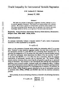
Figure 1 contains a directed acyclic graph (e.g., Pearl, 2000) representing these assumptions.

[FIGURE 1 ABOUT HERE.]

Core conditions 1-3 are required for estimators based on a fully specified parametric model for (X, Y, U, Z). However, for semi-parametric estimators the independence assumption can be replaced by, for example, conditional mean independence in which condition 2 becomes E(Y | X, U, Z) = E(Y | X, U) and condition 3 E(U | Z) = E(U). For simple linear structural models, condition 3 can be further relaxed: rather than the weaker E(U | Z) = E(U), the classical IV estimator comes from the stronger moment conditions

E ( ZU ) = E (U ) = 0 , where U = Y – β0 – Xβ1 under model (1).

(2)

The two-stage least-squares (2SLS) estimator is a

generalisation of (2) to include multiple exposures, more than one of which may be endogenous, which is identified provided there is at least one IV for each endogenous covariate. Stage one of 2SLS estimation involves fitting the ‘reduced-form’ model for the regression of X on Z using OLS, and using these predicted values in fitting linear model (1) at stage two. Provided the structural model is linear, the 2SLS estimator is consistent whether or not the true regression of X on Z is linear. Identification of treatment effect parameters under more general models has been considered by Imbens and Angrist (1994), Angrist et al. (1996) and Abadie (2003) among others; see also Tan (2006) for more recent work.

In this paper, we focus initially on IV estimators for non-linear regression models for binary Y, or more precisely, logistic and probit regression models. More generally, we focus on causal effects of X on Y. The consistency of maximum likelihood estimators for probit models is already well established

4

(e.g., Rivers and Vuong, 1988), but other estimators have also been proposed, based on the generalised method of moments (e.g., Angrist, 2001) and on potential outcome models: specifically, marginal structural models (e.g., Robins et al., 2000) and structural mean models (Robins, 1989; Robins, 1994). The attraction of these estimators is that full parametric specification of a model for (X, Y, U, Z) is not required.

Chesher (2008) has recently clarified the identification of structural models for discrete Y through a series of formal results, in which the assumptions embodied in the structural model for Y and X and core conditions 1-3 have been shown to be insufficient to identify the structural parameters. In the light of these results, we revisit all of these estimators to establish the context in which identification is obtained (or not). For the estimators based on potential outcomes, we do this by viewing potential outcomes models as semi-parametric structural models, and considering identification under simple models for the data generating process. From a practical perspective, we argue that, if identification cannot be achieved under simple structural models, the burden of proof shifts to any researcher using these methods to posit less simple but substantively plausible data generating processes under which it is.

The paper is organised as follows: In Section 2, structural and potential outcome models for binary Y are introduced, and the link between the two approaches is discussed. In Section 3, we summarise recent results on parameter identification for discrete Y and discuss their implications for IV estimation, and in Section 4 review likelihood-based estimation in the light of these results. In the remainder of the paper, we focus on semi-parametric estimators. The generalised method of moments is considered for binary structural models (Angrist, 2001; Johnson et al., 2008) in Section 5. The next two sections concern methods based on potential outcomes: in Section 6, the marginal estimator based on a marginal structural model (Ten Have et al., 2003); and second, in Section 7, estimators based on structural mean models (e.g., Vansteelandt and Goetghebeur, 2003; Hernán and Robins, 2006). In Section 8 we consider estimation under monotonic selection mechanisms, and in Section 9 we discuss the findings and draw conclusions.

2.

2.1.

Models for binary outcomes

Regression models

A generalised linear model for the regression of binary Y on X is b{µ ( x)} = β 0 + xβ1 ,

(3)

where µ(x) is the mean function and b(a) is a link function; C has again been omitted to simplify the subsequent development. We focus on the two most widely used models for binary Y, namely, the logistic model where b(a) = logit(a) = log{a/(1 – a)}, and the probit model where b(a) = Φ–1(a) is the

5

inverse cumulative distribution function (CDF) of the standard normal distribution. The logistic model is widely used in biomedical and social science disciplines because β1 is interpretable as a log odds ratio. In economics, it is the probit model that is most widely used; the slope parameter itself does not have an obvious interpretation, but it can be used to calculate the partial effect (PE). The PE of X at x* is defined to be the expectation of the derivative of the mean function at X = x* and is analogous to the ATE.

No explicit reference has been made to U in (3) because to do so is unnecessary if X is exogenous. However, if X is endogenous then it is important to understand the hidden role played by U. Using the notation introduced for linear model (1), a simple structural model for binary Y is given by

y = E (Y X = x, U = u )

= I ( β 0 + xβ 1 + u > 0),

(4)

where I(a) is the indicator function. It is again seen that the structural model wholly determines the observed value of the binary outcome. An alternative, the unobserved heterogeneity model, shall be discussed further on in Section 5. However, whatever structural model is chosen, an essential feature is that it must involve a non-smooth function to ensure the support of Y is the set {0, 1}.

If

X

is

exogenous

then

integrating

(4)

over

the

marginal

distribution

of

U

EU {E (Y X = x,U )} = E (Y X = x) = µ ( x) , and so the mean function of Y given X in (3) is correctly specified. The distribution of U is assumed to be normal for the probit model and logistic for the logistic model where, as well as constraining E(U) = 0, the scale of U is set arbitrarily so that Var(U) = 1 for normal U and Var(U ) = π 2 3 for logistic U. However, if X is endogenous then U is not

independent of X and EU | X =1{E (Y X = x,U )} ≠ µ ( x) .

2.2.

Potential outcome models

Potential outcome models distinguish between the selected exposure X and what happens if the exposure is set to χ by some hypothetical intervention or experiment. Instead of a structural model, a set of potential outcomes is defined for each unit in the study population. Units are indexed by i (which has been suppressed until now) and the potential outcome of unit i at exposure level χ is denoted by Yi ( χ ) , a suitably defined function of χ. In practice, only exposure level Xi is observed for unit i, and the observed outcome is related to the potential outcome by Yi = Yi ( X i ) ; this relationship is called the ‘consistency assumption’. The target of inference in the potential outcomes framework is a meaningful expectation taken over the entire population. For example, for binary X the ATE from Section 1 is E{Yi (1) − Yi (0)} , the causal risk ratio (CRR) is E{Yi (1)} E{Yi (0)} , and the causal odds ratio (COR) is 6

E{Yi (1)} E{1 − Yi (1)} . E{Yi (0)} E{1 − Yi (0)} As already stated, it is unnecessary to specify a parametric model for Yi(χ) in this framework. The endogeneity or unobserved confounding problem simply results in an association between Yi(χ) and Xi. However, throughout this paper we shall assume that Ui is the common cause behind this association, and thus we restrict attention to the wide range of non-ignorable selection models that are encountered in practice in disciplines like epidemiology and economics. With this in mind, we note how the simple binary structural model (4) can be written in terms of potential outcomes: suppress i and denote Yχ = Y ( χ ) , then y χ = E (Yχ U = u ) = I ( β 0 + χβ1 + u > 0) , where expectation over i has been replaced by expectation over the population distribution of U. As χ is fixed, integrating out U leads (if X is binary) to exp(β1) = COR under the logistic model. The potential outcomes models to be discussed in Sections 6 and 7 can thus be interpreted as semi-parametric, in that neither the error structure nor its distribution is explicitly specified.

IV estimators can therefore be developed in the potential outcomes context. Following Angrist et al. (1996), core conditions equivalent to 1-3 are: (i)

Pr( X = x Z = z ) is a nontrivial function of z,

(ii)

Conditional mean independence (CMI): E (Yχ Z = z ) = E (Yχ ) ,

(iii)

Exclusion restriction: Yzχ = Yχ ,

where Yzχ is the joint potential outcome, defined to be the outcome the participant would have obtained if her IV was set to z and exposure to χ. Note that the definition of the Yzχ implies that Z is a causal antecedent of X, and so the edge between Z and X in Figure 1 should be directed; see Hernán and Robins (2006) for a full discussion of the issue of causal and non-causal IVs.

Two other assumptions are often stated as core conditions within this framework (e.g., Angrist et al., 1996). These are that the selection mechanism for Z is ignorable (Rosenbaum and Rubin, 1983), and that the stable unit treatment value assumption (SUTVA) holds. The SUTVA requires that the potential outcomes for two or more people are independent, which is also implicit in the definition of the structural model, and is a commonly made working assumption. In randomised experiments, it is trivial to assume that Z is ignorable, but generally it is a strong assumption that is sometimes plausible only after conditioning on covariates. In the frameworks defined thus far, selection is ignorable only if Pr(Z = z | C = c, U = u, Y = y, X = x) = Pr(Z = z | C = c) or Pr(Z = z | C = c, Yχ = yχ, X = x) = Pr(Z = z | C = c).

7

3.

Parameter identification

We saw in Section 1 that the ATE is identified under the simple linear structural model (1) provided that IV Z satisfies the three core conditions. In contrast, identification for structural model parameters for discrete Y is a more precarious issue. Chesher (2008) considered this problem and his arguments are now summarised.

Identification requires that constraints implied by the model and the IV core conditions are sufficiently tight to ensure only one value of the model parameter is determined by the observed data. In general, the structural model is written Y = h(X, U*), where h is some function of the endogeneous covariate X and a normalised latent variable U*. Note that nothing more than this is assumed, and that the normalisation of U to be U* ~ Uniform (0,1) is for mathematical convenience, but makes no difference in practice: for example, the logistic model can be written Y = I{β0 + Xβ1 + logit(U*) > 0} using the integral probability transform. Within this framework, it has previously been shown that the IV core conditions are sufficient for identification if h is strictly monotonic (Chernozhukov and Hansen, 2005). However, the restriction on h for discrete Y is that it is weakly monotonic, that is, a stepfunction of U* for fixed X. For the logistic model, conditionally on X = x the step function can be written as Y = I {U x* > expit(− β 0 − xβ1 )} , where Ux∗ is a random variable following the conditional distribution of U* given X = x with CDF FU

*

|X

(τ x) = Pr(U x* ≤ τ ) , which is non-uniform and depends

on x, and expit( a ) = exp(a) {1 + exp(a )} is a convenient way to express the mean function of the logistic model.

Chesher (2008) shows that the constraints implied by core conditions 2-3 can be written E {Pr(U * ≤ τ | X , Z = z )} = τ ,

X Z =z

E {Pr(Y ≤ h( X ,τ ) | X , Z = z )} ≥ τ ,

X Z =z

E {Pr(Y < h( X ,τ ) | X , Z = z )} < τ ,

X Z =z

which can be expressed as functions of the model parameters and the observed data, namely, the conditional distributions of X given Z, and of Y given X and Z. In the simple double binary case, where both X and Z are dichotomous, the structural model is parameterised in terms of its two cut-off points, denoted by γ0 = expit(–β0) and γ1 = expit(–β0 –β1). It is shown that the observed data (nonparametrically) identify FU*|X(γ0|x = 0) and FU*|X(γ1| x = 1), that is, the data tell us something about one point of each conditional CDF. However, non-parametric identification requires that FU*|X(γ0| x = 1) and FU*|X(γ1| x = 0) are also uniquely determined, but Chesher (2008) shows that the data define only intervals within which each point must lie.

Therefore, identification comes about only by

parametrically specifying FU*|X.

8

4.

Likelihood-based estimation

From Section 3, we saw that identification of a binary structural model like (4) requires assumptions about the conditional distribution of U given X. A natural way to incorporate such assumptions is to use a likelihood function. The cost is that U given X is unobserved and maximum likelihood (ML) estimators can be highly sensitive to incorrect modelling assumptions. We now review ML estimators for probit models with continuous X (Rivers and Vuong, 1988). Normality has considerable benefits in terms of modelling the key assumptions, and guarantees consistency and asymptotic efficiency if these assumptions hold.

The probit estimator is based on the following pair of models Y = I ( β 0 + Xβ1 + U > 0), X = α 0 + Zα 1 + V ,

(5)

where the second part of (5) is called the reduced form model, and

 0   1 U    Z ~ N  ,  V   0   σ uv

σ uv   . σ v2 

It is important to distinguish the role played by the reduced-form model here to that for the 2SLS estimator. The linear reduced-form yields a consistent 2SLS estimator, whether or not the true reduced-form model is linear, whereas here the reduced-form model encodes additional assumptions that implicitly determine the crucial U given X distribution and identify the model. The ML estimator based on the model above is sensitive to this choice and will be inconsistent if it is incorrectly specified.

Rivers and Vuong (1988) further considered the properties of two simple estimators for probit models analogous to 2SLS. Both are conditional ML estimators because they involve replacing nuisance parameters by consistent estimators thereof (e.g., Severini, 2000). To recap, stage one involves fitting the reduced-form model (5) for X on Z, with stage two depending on which two-stage method is chosen: the ‘plug-in’ method involves replacing X in structural model (5) with its predicted value from fitting reduced-form model (5); alternatively, the ‘control variable’ method involves including an estimate of residual V in (5) as an additional covariate. Whereas the plug-in and control variable 2SLS estimators are equivalent, for probit models the control variable approach has a major advantage: the plug-in does not identify the structural parameter (only a scaled parameter is identified), while the

9

control variable method does identify the structural parameters by first identifying σuv (Rivers and Vuong, 1988). A semi-parametric control variable approach has been developed by Blundell and Powell (2004) using non-parametric estimation techniques to relax distributional assumptions.

Consistency of both conditional ML estimators hinges crucially on the reduced-form model being linear in V. For this reason, neither the plug-in nor the control variable methods produce consistent estimators for discrete X. For example, suppose X is binary and follows a probit reduced-form model X = I(α0 + Zα1+ V > 0) where V ~ N (0, σ v2 ) ; then the plug-in estimator is inconsistent because E (Y Z = z ) = E[ I {β 0 + I (α 0 + Zα 1 + V > 0) β 1 + U > 0} Z = z ] , and so the stage-two model cannot be a probit regression; similarly for the control variable method.

However, ML estimators can be

constructed by incorporating this reduced-form model directly into the likelihood, at the cost of losing the operational simplicity of the two-stage estimator.

In theory, the likelihood for any parametric model can be specified, but practical difficulties in specifying a suitable model occur if either U or V is non-normal. Despite this, conditional ML estimators have been proposed for logistic models. Palmer et al. (2008) use plug-in and control variable approaches for logistic models under a linear reduced-form model for endogenous X. The proposed estimators are developed with respect to the ‘unobserved heterogeneity’ structural model (see Section 5.1), rather than the simple structure in (4), for the important special case where the unobserved heterogeneity is normally distributed. However, the authors demonstrate neither estimator can be consistent, which is ultimately due to non-normality of U violating the conditions required for the stage-two likelihood to be a true conditional likelihood. Likewise, Nagelkerke et al. (2000) construct an IV estimator using arguments analogous to those for the control variable estimator above but for discrete X. This control variable approach is based on an additive error structure for the reduced-form model E(X | Z = z, V = v) = E(X | Z = z) + v, which leads to an inconsistent estimator if X is binary (see the arguments against this error structure in Section 5.3). The same estimator was considered for binary Y in a simulation study by Ten Have et al. (2003) and its bias was shown to be strongly related to the association between X and U.

5.

5.1.

The generalised method of moments (GMM)

GMM and the unobserved heterogeneity model

A family of estimators based on the generalised method of moments (GMM) has been developed in the econometrics literature. Johnson et al. (2008) give a concise overview of GMM estimators in a statistical context, while Wooldridge (2002, ch.14) gives a more complete account. GMM estimation is a generalisation of the method of moments to allow for one or more endogenous covariates, where multiple IVs may be available for each. Situations involving only one endogenous exposure and one

10

IV are considered here, so strictly speaking only method of moments estimators are considered, but this is done without loss of generality.

GMM estimators for non-linear structural models exploit the condition E(U | Z) = E(U) = 0 (which implies E(ZU) = 0 as in moment condition (2)). Thus, to develop a GMM estimator it must be possible to express U as the error for a logistic or probit structural model and to substitute this expression into the moment condition. Models satisfying this condition are called ‘mean separable’. Linear models are clearly mean separable because u = y – β 0 – xβ 1. However, it is clear that the structural models for binary Y are not mean separable because they involve the indicator function.

A strategy to obviate the presence of the indicator function is to consider an alternative error structure. For instance, the structural model y = E (Y X = x, W = w, U = u ) = I ( β 0 + xβ 1 + w + u > 0) ,

(6)

is obtained by replacing U in simple structural model (4) with W + U, where W represents omitted variables associated with X and Y, and U represents the usual error term associated only with Y. Model (6) is called a mixed effects or unobserved heterogeneity model. If U is assumed to follow a logistic distribution then E (Y X = x, W = w) = expit(β 0 + xβ 1 + w) ,

(7)

recalling that expit( a ) = exp(a ) {1 + exp(a )} . Note that (7) does not wholly determine observed outcome y, it is the conditional probability that Y = 1 given X and (unobserved heterogeneity) W. Unobserved heterogeneity model (7) cannot be represented using the formulation of Chesher (2008) discussed in Section 3. However, as shall become apparent here and further on, this does not solve the identification problem for semi-parametric estimators because the resulting mean function is not mean separable. By changing the error structure, the interpretation of β 1 in (6) has also changed: it is now the conditional log-odds ratio given W = w.

In econometrics, the target parameter for unobserved

heterogeneity models like (6) is the ‘average partial effect’ (APE) rather than the PE, defined as the expected value of the PE over the distribution of W for a fixed value x*. We now consider two approaches exploiting this alternative error structure.

5.2.

A rare event approximation

An exponential mean model is E (Y X = x, W = w) = exp(β 0 + xβ1 + w) , 11

(8)

which is used for constructing estimators for the risk ratio for non-negative Y (see Angrist (2001) and Section 8). If the outcome event probability is reasonably considered to be ‘small’, then this is superficially a reasonable approximation for logistic model (7). Once more, GMM estimators have already been applied to endogenous Poisson regression models with exponential mean functions; for example, Mullahy (1997) constructs an estimator based on the ‘multiplicative’ moment condition ~ ~ E (U Z = z ) = 0 ⇒ E ( ZU ) = 0 ,

(9)

~ where U = Y exp(−α − Xβ 1 ) − 1 and α = β 0 + log[E{exp(W)}]. Under regularity conditions, the GMM estimator is consistent for α and relative risk β 1, but not β 0. However, the confounding of β 0 poses no problem if one targets the APE, which equals exp(α){exp(β 1) – 1} under exponential mean model (8). It would appear to follow that an estimator based on (9) is a sensible way to proceed if the event probability is rare. However, if we assume that exp(β0 + xβ 1 + w) ∈ (0, δ) for all (x, w) for some fixed (β 0, β 1) where δ is close to zero, then ~ E (U Z = z ) = O (δ ) , under logistic model (7), which indicates that the moment condition error is of the same order as the event probability itself. Contrast this with the situation if X is exogenous: if exponential mean model (8) is true then a consistent estimator comes from the ‘additive’ (i.e. Poisson first-order) moment condition E{Y − exp(β 0 + Xβ1 ) X = x} = 0 . Under the logistic model (7), E{Y − exp(β 0 + Xβ1 ) X = x} = O(δ 2 ) , in other words, the moment condition error is an order smaller than the event probability itself. (See Appendix 1 for a more detailed argument.) It follows from this that, if X is endogenous, the bias of the estimator will increase quickly as the event becomes less rare. Conversely, in cases where the bias is small then the outcome event must be very rare, thus requiring large sample sizes to ensure the estimator is accurate and has an approximately normal sampling distribution.

5.3.

Additive error structure approximation

Johnson et al. (2008) propose a GMM estimator based on E (Y X = x,W = w) = expit(β 0 + xβ 1 ) + w .

(10)

The moment conditions follow from substituting the residual into moment conditions E(W) = E(ZW) = 0. However, the structural model implied by this model is implausible because the support of W is

12

bounded by X (i.e., –expit(β0 + xβ 1) ≤ w ≤ 1 – expit(β0 + xβ 1)), and so (10) is structurally implausible because it contradicts the implicit assumption that W is causally antecedent to X and Y. Another criticism is that the effect of the omitted variables is not ‘symmetric’ in the sense that the effect on Y of omitted W is on a different scale to that of X (Mullahy, 1997).

Johnson et al. (2008) do not argue that (10) is plausible, but that it is a first-order approximation of unobserved heterogeneity model (7); that is, expit(β 0 + xβ 1 + w) ≈ µ(x) + wυ, where µ(x) = expit(β 0 + xβ 1), υ = µ ( x ){1 − µ ( x )} and x = E ( X ) , which is based on two successive first-order Taylor series expansions: first an expansion of expit(β 0 + xβ 1 + w) around w = 0, and second of µ(x){1 – µ(x)} around x = x . However, the first-step approximation here is poor: consider the first approximation but do not drop the second-order term, then the moment condition becomes E{Y − µ ( X ) Z = z} ≈ E{expit( β 0 + Xβ 1 + W ) − µ ( X ) Z = z}

= E[Wµ ( X ){1 − µ ( X )} + W 2 µ ( X ){1 − µ ( X )}{1 − 2 µ ( X )} 2 Z = z ]. Clearly, to equal zero this approximation depends heavily on independence between X and W, and the W2 term indicates that second-order moments including the variance of W must also be small. The

second-step of the approximation is additionally restrictive, and taken together rules out GMM based on (10) as a good approximation in general.

6.

The marginal estimator

In this section, we consider estimators based on the potential outcomes approach, namely, marginal structural models, and go on to consider estimators based on structural mean models in Section 7. As discussed in Section 2.2, we treat both of these approaches as semi-parametric because neither involves full parametric specification of U in the structural model. We now consider the behaviour of these potential outcomes estimators under the structural models already introduced, simple model (4) and unobserved heterogeneity model (6). If identification and consistency cannot be obtained under such simple models, we argue that these estimators are not generally identified, at least without further (possibly application-specific) assumptions.

Ten Have et al. (2003) propose a ‘marginal’ estimator based on a marginal structural model (MSM) for binary outcomes. Generally, a MSM has the form E (Yχ ) = gψ ( χ ) (e.g., Robins et al., 2000; Hogan and Lancaster, 2004). Ten Have et al. (2003) consider the logistic MSM

E (Yχ ) = expit(ψ 0 + χψ 1 ) ,

13

(11)

recalling that χ is used to denote that exposure has been set by external intervention rather than by the selection mechanism that generated the study data.

Dependence on covariates comes through

extending (11) to include C in the linear predictor, with the proviso being that the effect of exposure in (11) is now covariate-conditional. Due to (11) (and its probit equivalent) being non-collapsible (e.g., Greenland et al., 1999), this effect does not equal the population effect of X, which can only be estimated by averaging the covariate-conditional effects over the sample covariate distribution.

The marginal estimator comes from the moment condition ~ E[{Z − E ( Z )}U ] = 0 ,

(12)

~ where U = Y − gψ ( X ) is the MSM ‘residual’. Clearly, this approach is analogous to the GMM ~ ~ estimator from Section 5.2: if U is a residual such that E (U ) = 0 then (12) is analogous to solving ~ ~ E (U Z = z ) = 0 and hence E ( ZU ) = 0 . Ten Have et al. (2003) proposed that (12) holds for an unobserved heterogeneity model (6) with only two further relatively weak conditions on the IV. Before inspecting this result more closely, we shall make some observations.

Strictly, the only distributional assumptions about U and W made by unobserved heterogeneity model (6) (or whatever error structure is assumed) are that the underlying structural model leads to (11) following integration. However, Ten Have et al. (2003) assume that U in (6) is logistic to obtain a logistic unobserved heterogeneity model (7).

Generally, this model is non-collapsible, so their

solution was to choose normal W because the resulting MSM (11) is approximately logistic. In fact, this is an unnecessary restriction because it is done to keep the parameters of conditional model (7) as target parameters. The parameters of MSM (11) are simply those of a marginal model, and their relationship with those of conditional (on W) model (7) is analogous to that between ‘cluster-specific’ and ‘population averaged’ models (e.g., Neuhaus et al., 1991). Nothing has been lost by this change of focus: ψ1 is directly interpretable as the causal odds ratio (or covariate-conditional causal odds ratio) and thus a more appropriate target parameter than β 1 in (7). Returning to consistency, close inspection of the consistency proof by Ten Have et al. (2003) reveals that either of two further strong conditions are required, namely, X ╨ W | Z or E(Yχ | W = w) = E(Yχ) (╨ is the symbol for conditional independence). We present a formal result and a justification of this in Appendix 2. Both of these conditions correspond to X being exogenous, and so consistency is obtained only in trivial circumstances. In essence, without either of these conditions holding it follows ~ ~ that E (U Z = z ) ≠ 0 , and so U is not a ‘proper’ residual and the analogy with the GMM estimator breaks down.

In practice therefore, the marginal estimator is at best an approximation.

14

The

simulation results presented by Ten Have et al. (2003) demonstrate that the bias depends on the association between X and W and between W and Y, and this is not simply finite sample bias.

7.

Structural mean models (SMMs)

Structural mean models (SMMs) are a class of semi-parametric models for estimating causal parameters for the exposed population, which were originally developed for the analysis of randomised controlled trials affected by non-ignorable non-compliance (e.g., Robins, 1989; Robins, 1994; Hernán and Robins, 2006). Vansteelandt and Goetghebeur (2003) introduced the family of generalised SMMs that includes logistic and probit SMMs as special cases along with a class of estimators for these models; Robins et al. (1999) originally proposed the logistic SMM.

Generally, a SMM has the form b{E (Y X = x, Z = z )} − b{E (Y0 X = x, Z = z )} = ηψ ( x, z ) ,

where b(a) is a link function and ηψ ( x, z ) is a parametric function constrained such that ηψ (0, z ) = 0 for all z. Covariates C are included by a suitable specification of η, which is often parametric to prevent the ‘curse of dimensionality’ leading to poorly performing estimators. SMMs are most easily explained for the special case where X and Z are both binary, and so X and Z are taken to be binary throughout this section. Three examples of saturated SMMs with one parameter for each combination of (x, z) are given below:

Example 7.1a: The additive SMM is E (Y X = x, Z = z ) − E (Y0 X = x, Z = z ) = xψ za .

It follows that ψ za = E (Y1 X = 1, Z = z ) − E (Y0 X = 1, Z = z ) = ATE( X = 1, Z = z ) , namely, the ATE among the exposed population with Z = z.

Example 7.1b: The multiplicative SMM is log{E (Y X = x, Z = z )} − log{E (Y0 X = x, Z = z )} = xψ zm . It follows that exp(ψ zm ) = CRR( X = 1, Z = z ) , namely, the CRR among the exposed population with Z = z.

Example 7.1c: The logistic SMM (Vansteelandt and Goetghebeur, 2003) is: 15

logit{E (Y X = x, Z = z )} − logit{E (Y0 X = x, Z = z )} = xψ zl . It follows that exp(ψ zl ) = COR( X = 1, Z = z ) , namely, the COR among the exposed population with Z = z.

The SMM estimator comes from exploiting the moment conditions implied by the randomisation, or conditional mean independence (CMI), assumption (core condition ii). From the CMI assumption, it follows that

E {E (Y0 X , Z = 1)} = E {E (Y0 X , Z = 0)} = E (Y0 )

X |Z =1

X | Z =0

(13)

⇒ E {E (Y0 X , Z = 1)} − E {E (Y0 X , Z = 0)} = 0, X |Z =1

X |Z = 0

where E(Y0 | X = x, Z = z) = b–1[b{E(Y | X = x, Z = z)} – xψz], with superscripts dropped here to indicate generic parameters for any of the SMMs presented above. An important assumption regarding SMMs is that of ‘no effect modification by Z’ (NEM) or ψz = ψ. Without the NEM assumption the SMM estimator is not identified (Robins and Rotnitzky, 2004). The crucial importance of this assumption shall be considered again further on. Estimators for the three SMMs considered in Example 7.1 under the NEM assumption are given below:

Example 7.2a: For the additive SMM in Example 7.1a, the SMM estimator can be written

ψˆ a =

E (Y Z = 1) − E (Y Z = 0) E ( X Z = 1) − E ( X Z = 0)

,

which equals the classical IV estimator from Section 1 in the case where both X and Z are binary.

Example 7.2b: For the multiplicative SMM in Example 7.1b, the SMM estimator comes from solving E{Y exp(− Xψ m ) Z = 0} = E{Y exp(− Xψ m ) Z = 1} .

(14)

Hernàn and Robins (2006) note that (14) has a closed form solution (see also Angrist (2001, eq.21)), given by exp(ψˆ m ) =

E ( XY Z = 1) − E ( XY Z = 0) E{(1 − X )Y Z = 1} − E{(1 − X )Y Z = 0}

.

(15)

Example 7.2c: For the logistic SMM in Example 7.1c, the SMM estimator comes from solving 16

E expit[logit{E (Y X , Z = 0)} − Xψ l ] = E expit[logit{E (Y X , Z = 1)} − Xψ l ] ,

X |Z = 0

X | Z =1

(16)

which does not have a closed-form solution.

An important distinction between the SMMs for binary Y (logistic and probit) and other SMMs is that the moment condition is not a function of the observed data (Y, X, Z) alone, and so cannot be estimated using the usual SMM estimators (Robins, 1999). SMMs for binary Y depend additionally on the ‘association model’ E(Y|X = x, Z = z).

In fact, this dependence on the association model for

identification can be seen as a semi-parametric expression of the result in Section 3: for example, under structural model (4) the association model is E (Y X = x, Z = z ) = =

E

E (Y | X = x, U , Z = z )

E

E (Y | X = x, U )

U | X = x ,Z = z U | X = x ,Z = z

= ∫ E (Y X = x, U = u )dFU | X ,Z (u | x, z ), u

where FU|X,Z(u | x, z) = Pr(U ≤ u | X = x, Z = z). In other words, identification depends on specification of U given X and Z (and hence U given X because FU|X(u | x) = E{FU|X,Z(u | x, Z) | X = x}). Vansteelandt and Goetghebeur (2003) developed an estimator for the logistic SMM that takes advantage of user-specified parametric assumptions about the association model. For the simple saturated models considered here, this identifying restriction is not particularly strong, but generally, and particularly if covariates are introduced, parametric assumptions on the association model are required to avoid the curse of dimensionality and are thus more important. The simplest example of such an estimator is based on a logistic SMM and a logistic association model, and so is called ‘double logistic’ by Vansteelandt and Goetghebeur (2003).

7.1.

The connection between SMM and GMM estimators

There is a close correspondence between the SMM estimators and the GMM estimators introduced in Section 5, which while obvious for linear models deserves elaboration for the non-linear case.

First, consider the link between the moment conditions of the multiplicative SMM and the multiplicative GMM moment condition (9) if exponential structural model (8) is true.

Under

exponential mean model (8), E (Y0 ) = E{exp( β 0 + W )} = exp(α ) where α is defined in (9). Now consider the moment conditions for the multiplicative SMM, and use the first expression of the CMI assumption from (13); substituting gives E{Y exp(− Xψ m ) Z = z} = exp(α ) ,

17

which

leads

immediately

to

multiplicative

GMM

moment

condition

(9)

because

E{Y exp(−α − Xψ m ) − 1 Z = z} = 0 ⇒ E[ Z {Y exp(−α − Xψ m ) − 1}] = 0 .

Generally, rather than the structural model residual used by GMM, the SMM estimator is based on another residual. For the logistic SMM, the residual is E(Y0 | X, Z = z) – E(Y0) = E(Y0 | X, Z = z) – E(Y0 | Z = z) = 0, whereas the multiplicative SMM is based on E(Y0 | X, Z = z)/E(Y0 | Z = z) – 1 = 0. The first of these residuals can be regarded as that of a (non-linear) projection of Z onto Y0, whose expectation over X given Z is zero. The second has the same interpretation but works on a multiplicative scale. Under the SMM, the residual can be written as a function of model parameters and observed data, and a consistent estimator derived if the moment conditions ensure identification.

For Z with a large finite or infinite support set, the system of SMM moment conditions is given by E (Y0 Z = z1 ) = E (Y0 Z = z 2 ) for all observed z1 ≠ z2 in the support. The large number of resulting moment conditions is clearly problematic for constructing an estimator. One way forward is thus to take an approach analogous to GMM by defining a structural model for E(Y0), which permits ~ construction of the projection residual like that just discussed (i.e., where E (U Z ) = 0 ), from which it ~ follows that an estimator can be based on the moment condition E ( ZU ) = 0 (or some variation thereof). Before this approach can be considered for binary Y, however, more germane problems of parameter identification must be overcome.

7.2.

Binary structural models, effect modification, and identification

To be useful, any SMM must be congenial with a sensible structural model. For example, if the exponential mean model (8) holds then we would expect the multiplicative SMM moment conditions to produce a consistent estimator. Indeed, this is the case under model (8):

exp(ψ zm ) =

exp(β 0 + β1 ) exp(β 0 )

E

{exp(W )}

W | X =1, Z = z

E

{exp(W )}

=

exp(β 0 + β1 ) E {exp(W )} W | X =1

exp(β 0 ) E {exp(W )}

W | X =1, Z = z

= CRR( X = 1),

W | X =1

because clearly the expectations of exp(W) cancel out. Thus, the NEM assumption holds whatever the selection mechanism, and so exp(ψ zm ) = exp(ψ m ) (and the additional benefit that CRR(X = 1) = CRR = exp(β 1)). Unfortunately, the situation for binary structural models is much less positive. Consider either simple structural model (4) or unobserved heterogeneity model (6). In the latter case, the multiplicative SMM does not satisfy the NEM assumption because

exp(ψ zm ) =

{expit(β 0 + β 1 + W )}

E

W | X =1, Z = z

E

{expit(β 0 + W )}

W | X =1, Z = z

18

depends on Z unless trivially W

╨

Z | X = 1 (╨ is again the conditional independence symbol).

Similarly, the logistic SMM does not satisfy the NEM because COR(X = 1, Z = z) depends on z too, with the same results holding for structural model (4). The same problem as with GMM is thus apparent: W is not mean separable for logistic (or probit) structural models, and so it follows that neither the additive, multiplicative nor the logistic SMMs identify their respective causal effects among the exposed due to failure of the NEM. Neither the additive, multiplicative nor logistic SMMs are identified because the NEM assumption fails. Didelez et al. (2008) demonstrate inconsistency of the multiplicative SMM for binary Y in an extensive numerical study.

Robins and Rotnitzky (2004) investigate the identification of SMMs for binary Y, highlighting the key role played by the NEM assumption. At a fundamental level, the NEM assumption is required to reduce the number of unknowns: for example, in the simple example above, without the NEM assumption there are two unknowns (ψ0, ψ1) but only one moment condition. Furthermore, although only simple structural and reduced-form models have been considered here, we do not believe that plausible structural models for binary Y exist satisfying the NEM assumption. This opinion is supported elsewhere: “[the NEM] assumption is unrealistic because [the exposed] subpopulations [defined by Z] are likely to be quite different with regard to modifiers of the effect of active treatment on the outcome of interest” (Robins and Rotnitzky, 2004, p. 778).

Robins and Rotnizky (2004) show that identification can be obtained by constraining one or more of the ψz parameters. For example, in the randomised clinical trial context, the treatment restriction “no treatment among the controls” corresponds to forcing Pr(X = 0 | Z = 0) = 1, and has been used in a number of studies (e.g., Nagelkerke et al., 2000; Ten Have et al., 2003; Vansteelandt and Goetghebeur, 2003, 2005). Under this ‘treatment restriction’ assumption, ψ1 is identified because ψ0 is fixed (at an extreme value corresponding to a non-existent effect), even if the NEM assumption does not hold. However, while reasonable for many randomised controlled trials, the exposure restriction assumption is too strong for observational studies.

7.3.

An alternative estimator

Robins and Rotnitzky (2004) propose an estimator that addresses this identification problem. It is based on an alternative parameterisation of the association model. Semi-parametric theory is used to find the influence functions for a regular asymptotically linear estimator of the SMM parameters and of a parametric model for the observed data (Y, X, Z). As with the covariance estimators for the SMMs, a semi-parametric covariance estimator is used to allow for non-normality of these estimators in finite samples (e.g., Robins and Ritov, 1997). The estimator involves two stages: the first stage is crucial because it identifies the (non-SMM) nuisance parameters using parametric assumptions in much the same way as maximum likelihood, while stage-two allows semi-parametric specification of 19

the SMM. Semi-parametric consistency and efficiency is obtained only if the modelling assumptions are correct. However, unlike maximum likelihood estimators, these estimators are ‘locally robust’ in that one can test for ψz = 0 even if the parametric models are misspecified, although the power of this test will be compromised by misspecification.

8.

Monotonic selection

Given the problems encountered with binary Y thus far, it remains to clarify what actually can be estimated without fully specifying parametric structural and reduced-form models.

A possible

approach is to assume that selection is monotonic in Z. To define monotonic selection, it is necessary to define the potential outcome Xi(z) ≡ Xz (c.f. Section 2.2). In the case of binary Z and X, the study units fall into one of four groups: 1. Compliers: X0 = 0 and X1 = 1. 2. Always-takers: X0 = 1 and X1 = 1. 3. Never-takers: X0 = 0 and X1 = 0. 4. Defiers: X0 = 1 and X1 = 0. Note that these groups are defined using what the study unit would have selected if its IV had taken another value, and so is an unobservable counterfactual. A monotonic selection mechanism requires that Xz is a non-decreasing function of Z (or non-increasing, depending on the labelling). In this example, monotonic selection implies the set of defiers is empty with probability one.

The reduced-form model for binary X is clearly a special case of the general class of monotonic selection mechanisms because X z = I (α 0 + zα 1 + V > 0) implies that X1 ≥ X0 or X1 ≤ X0, depending on the sign of α1. However, a heterogeneous effect version, corresponding to the data generating process X z = I {α 0 + zα 1 + I ( z = 0)V0 + I ( z = 1)V1 > 0} , where Vz is drawn differentially depending on Z, is not monotonic.

Without including covariates, the additive SMM estimator is consistent for the ‘local’ ATE (LATE), defined LATE = E (Y1 − Y0 X 1 > X 0 ) , if selection is monotonic (Imbens and Angrist, 1994; Angrist et al., 1996); this parameter is also known as the ‘complier’ average causal effect (CACE).

The

parameter is local because the conditioning set refers to the complier group consisting of those whose selection was modified by the IV. Previously, the IV estimator has been considered together with the linear structural model (1), where it was shown to be consistent for the ATE rather than the LATE. Identification of the ATE is achieved in this case by assuming model (1) is linear, and additionally that Yi (1) − Yi (0) = β1 for all i (using the notation from Section 2.2). Imbens and Angrist (1994) showed that the IV estimator is consistent for the LATE without either of these assumptions if selection is 20

monotonic.

Hence, the LATE can be identified if Y is binary using these assumptions under

monotonic selection.

In the same way, Angrist (2001) showed that multiplicative SMM (15) is consistent for the local CRR, defined LRR = E (Y1 X 1 > X 0 ) E (Y0 X 1 > X 0 ) . In contrast, the logistic SMM estimator is inconsistent for the local COR (LOR) unless the additional assumption that E(Y1 | X1 > X0) = E(Y1 | X1 = X0 = 1) is made (see Appendix 3). Such an assumption is no less heroic than NEM and so is of little practical use. However, Abadie (2003, eqs.3-4) shows that a consistent estimator for the LOR is {E (YX Z = 1) − E (YX Z = 0)} [ E{(1 − Y ) X Z = 1} − E{(1 − Y ) X Z = 0}] [ E{(1 − X )Y Z = 1} − E{(1 − X )Y Z = 0}] [ E{(1 − X )(1 − Y ) Z = 1} − E{(1 − X )(1 − Y ) Z = 0}]

.

Hence, local averages with causal interpretations can be identified under monotonic selection.

If covariates are included, Abadie (2003) proposes a weighted estimator to identify the parameters of the local average response function E(Yx|X = x, C = c), i.e., including covariates, either semiparametrically via least-squares or parametrically using maximum likelihood.

Estimates of the

(covariate-conditional) LATE, LRR or LOR can then be constructed using this approach.

Imbens and Rubin (1997) set out a Bayesian framework for estimation of treatment effects among the complier, always-taker and never-taker groups under a monotonic selection mechanism. Widening the focus from effects in the complier group (LATE) to all three non-defier groups is achieved by incorporating parametric assumptions. Hirano et al. (2000) apply these ideas, and extend them to allow for covariates, to a randomised controlled trial with binary outcomes.

9.

Discussion

In this paper, we have brought together estimators for causal effects involving binary outcomes from structural modelling and potential outcomes frameworks by treating the potential outcomes models as semi-parametric structural models. Thus, our focus is on non-ignorable selection mechanisms as they are conceptualised in applied disciplines like epidemiology and economics, i.e., driven by unobserved confounders or omitted variables correlated with the exposure. The crucial result regarding nonidentification is due to Chesher (2008), who has shown that the identification problem affects all structural models for discrete outcomes, and estimators must incorporate further modelling assumptions to identify causal effects. We have explicated the implications of this result for semiparametric estimators within our framework.

21

As is well known, ML estimators achieve identification through additional specification of the reduced-form model relating X and Z (and C). Unlike the 2SLS case for linear models, the reducedform model is crucial to ML estimator consistency: the choice of logistic or probit structural model is thus now crucial, as well as the specification of the reduced-form model. The normal distribution has attractive properties conducive to a tractable, well-behaved ML estimator that can be fitted using software such as Stata (StataCorp, 2007). More generally, the flexibility of likelihood methods is limited only by the modelling tools at ones disposal and the computational issues faced. Normality is also crucial to conditional likelihood methods, and consistency of the control variable two-stage probit estimator. However, consistent conditional likelihood estimators can be inefficient, and cannot be derived at all if X is discrete, which unfortunately includes the important binary exposure case.

GMM estimators cannot be consistent because models for binary Y are not mean separable. Simply assuming the model residual is additive or multiplicative with respect to the mean function is structurally implausible because it implicitly assumes the support of U depends on X, despite an implicit assumption of the analysis being that U is a causal antecedent of X. Extending the error structure to two latent variables U and W fails to overcome this problem because the resultant mean functions are not mean separable. Johnson et al. (2008) argue that the GMM estimator is valid under certain conditions, but we show that these conditions are too restrictive in practice to yield a useful estimator. Another approach if the outcome event is rare is to approximate the logistic mean function with an exponential mean model. However, we argue that the multiplicative GMM estimator is consistent only for very rare outcomes (and so requires very large sample sizes) and that its accuracy deteriorates quickly as the event probability increases.

In Sections 6 and 7, two estimator classes based on the potential outcomes framework were considered. The marginal estimator proposed by Ten Have et al. (2003) is seen to be closely related to the GMM estimator. It is based on a ‘pseudo’-residual from a suitable marginal structural model, but we have shown that it is only consistent if X is exogenous. The SMM estimators are potentially consistent for causal parameters defined among the exposed population, but identification hinges on the no effect modification (NEM) by Z assumption (Robins and Rotnitzky, 2004). We highlighted how the SMM estimator is a special case of GMM based on a suitably defined residual, but that the NEM assumption does not hold even for simple structural models for binary Y. As with GMM, nonidentification and the failure of the NEM assumption come about due to the binary structural model not being mean separable.

Identification through treatment-restrictions like no treatment among

controls is only plausible for some randomised controlled trials, and almost certainly implausible for observational studies.

In the absence of parametric assumptions, a more realistic aim is to focus on local parameters under the assumption of a monotonic selection mechanism. Imbens and Angrist (1994) show how the 22

classical IV estimator can always estimate the local average causal effect, no matter what the structural model (including no linearity or causal effect heterogeneity restrictions), provided that selection is monotonic. The monotonicity assumption is unverifiable and has attracted severe criticism (Dawid, 2000), but it is possibly less controversial if viewed as placing a very general restriction on the reduced-form model.

Local estimators including exogenous covariates can be constructed from

theorem 3.1 of Abadie (2003). Van der Laan et al. (2007) has proposed another approach by defining alternative target parameters, and constructs estimators for these using semi-parametric estimating equations.

Finally, it is important to recognise that not all researchers will accept the framework within which potential outcomes models are taken to be semi-parametric structural models. We feel that the challenge for applied researchers is to make assumptions about the structural model and selection process that are grounded in substantive knowledge of their studies, and that our framework is the most obvious and transparent way in which to do this. Certainly, it is possible that identification can be obtained for potential outcomes models based on alternative assumptions, such as equating outcome averages for compliers and non-compliers (e.g., Ten Have et al., 2003); but the challenge to the researcher is then to posit plausible structural and selection models satisfying these assumptions, rather than to make them for mathematical reasons alone.

Appendix 1: Rare event approximation Suppose that we wish to use the rare event approximation E (Y X = x, W = w) = expit(β 0 + xβ1 + w) ≈ exp(β 0 + xβ1 + w) , and construct a GMM estimator based on moment condition (9). In other words, let q(x,w) = exp(β 0 + xβ 1 + w), take (β 0, β 1) to be fixed and set E{exp(W)} = 1 ⇒ α = β 0. Assuming that all q(x,w) ∈ (0, δ), rewrite (9) as

 E (Y X ,W , Z = z ) − exp(β 0 + Xβ1 )   Y − exp(β 0 + Xβ1 )  E Z = z = E  . exp( β 0 + Xβ 1 )  exp(β 0 + Xβ1 )  X ,W |Z = z   Now write expit(β 0 + xβ 1 + w) = q/(1 + q), where q = q(x,w); a second-order Taylor series expansion of q/(1 + q) around q = 0 gives E (Y X = x, W = w, Z = z ) = expit(β 0 + xβ1 + w) = q − q 2 + O (q 3 ) , for small q. We can ignore the remainder term and it follows that

 E (Y X ,W , Z = z ) − exp(β 0 + Xβ1 )  W W W E   = X ,WE|Z = z (e − 1) − X ,WE|Z = z (e q ) = − X ,WE|Z = z (e q ), exp( β 0 + Xβ 1 )  

X ,W | Z = z

where E (eW q Z = z ) ≤ δE (eW ) = δ and so the error is O(δ). In other words, the moment condition is only as accurate as the event probabilities are rare. Contrast this with the exogenous case, where the additive moment condition error is

23

E{Y − exp(β 0 + Xβ 1 ) X = x} = E {(eW − 1) exp(β 0 + Xβ 1 ) − e 2W exp(2 β 0 + 2 Xβ 1 )} = O (δ 2 ) W |X =x

which is an order smaller than the rare event approximation itself.

Appendix 2: Consistency of marginal estimator Result 1: Suppose MSM E(Yχ) = gψ(χ) is obtained under some structural model such as (7), where Yχ = hψ(χ,w,u), E(Yχ | W = w) = kψ(χ,w) and (U, W) follow some unspecified joint distribution. Then consider the conditions: (i) Y = YX = ∑x I(X = x)Yx; (ii) W ╨ Z; (iii) E(Yχ | X, W, Z) = E(Yχ |W, Z); (iv) X

╨

W | Z; and (v) kψ(χ,w) = gψ(χ). If either (a) conditions (i-iii,iv) hold, or (b) conditions (i,iii,v)

hold, then moment condition (12) is true; otherwise it does not. (Note that

╨

is the symbol for

conditional independence here.) Proof: We suppose that Yχ ≡ E(Yχ | W = w, U = u) = h(χ, w, u) is structural model (7), such that h(χ, w, u) = E(Y | X = χ, W = w, U = u) = Y, E(Yχ | W = w) = E{h(χ, w, U)| W = w} = kψ(χ, w) and E(Yχ ) = E{kψ(χ, W)} = gψ(χ) is the MSM. The expected value of the inner part of the estimating equation conditional on Z is E{Y − gψ ( X ) Z = z} = E (Y Z = z ) − E{gψ ( X ) Z = z} . To show (a), consider the second term of the right-hand side: E{gψ ( X ) Z = z} = E{∑ x I ( X = x) gψ ( x) Z = z} = ∑x Pr( X = x Z = z ) gψ ( x) = ∑x Pr( X = x Z = z ) E{kψ ( x, W )} = ∑x ∫ Pr( X = x Z = z ) Pr(W = w) E{hψ ( x, U , w)}dw U

w

= ∑x ∫ Pr( X = x Z = z ) Pr(W = w) E{E (Y X = x, W = w, U )}dw, from(i) U

w

= ∑x ∫ Pr( X = x Z = z ) Pr(W = w) E{E (Y X = x, W = w, U , Z = z )}dw, redundancy U

w

= ∑x ∫ Pr( X = x, W = w Z = z ) E (Y X = x, W = w, Z = z )dw, from (ii, iv) w

= E (Y Z = z ), and so it follows that E{Y – gψ(X) | Z = z} = 0, as required provided gψ(χ) is correct. To show (b) follow Ten Have et al. (2003, appendix A), who give an alternative proof assuming only (i) and (iii). Following their argument

E{Y − gψ ( X ) Z } = E E E{Y − gψ ( X ) X , W , Z } W |Z X |Z ,W

= E E {E (Y X , W , Z ) − gψ ( X )} W |Z X |Z ,W

= E E {E (YX X , W , Z ) − gψ ( X )} from (i) W |Z X |Z ,W

= E E {E (YX W , Z ) − gψ ( X )} from (iii) W |Z X |Z ,W

= E

W |Z

∑ Pr( X = x W = w, Z ){k

ψ

x

24

( x, W ) − gψ ( x)},

which is zero if condition (v) holds, that is, kψ(χ, w) = gψ(χ), or if condition (iv) holds. By inspecting the first equality of (A4) in Ten Have et al. (2003), it can be seen that their proof makes this unstated assumption.

Appendix 3: Identification of the LOR by the logistic SMM To show this, let ψˆ = ψˆ and write the generalised SMM estimator of Vansteelandt and Goetghebeur l

(2003) as E (b −1[b{E (Y X , Z = 1)} − Xψˆ ]) = E (b −1[b{E (Y X , Z = 0)} − Xψˆ ]) ,

X |Z =1

X |Z = 0

where b(a) = logit(a). Expanding Pr( X = 0 Z = 0) E (Y X = Z = 0) + Pr( X = 1 Z = 0)b −1[b{E (Y X = 1, Z = 0)} − ψˆ ] = Pr( X = 0 Z = 1) E (Y X = 0, Z = 1) + Pr( X = 1 Z = 1)b −1[b{E (Y X = Z = 1)} − ψˆ ], and rewriting as Pr( X 0 = 0) E (Y0 X 0 = 0) + Pr( X 0 = 1)b −1[b{E (Y1 X 0 = 1)} − ψˆ ] = Pr( X 1 = 0) E (Y0 X 1 = 0) + Pr( X 1 = 1)b −1[b{E (Y1 X 1 = 1)} − ψˆ ], similar arguments to those used for the proportional LATE gives Pr( X 1 = 1)b −1[b{E (Y1 X 1 = 1)} − ψˆ ] − Pr( X 0 = 1)b −1[b{E (Y1 X 0 = 1)} − ψˆ ] E( X 1 − X 0 )

= E (Y0 X 1 > X 1 )

It can clearly be seen that, because b is a non-separable function, generally the left-hand side is determined by ‘always takers’ as well as compliers and cannot admit a local interpretation (because E(Y1 | X0 = 1) = E(Y1 | X0 = X1 = 1) and E(Y1 | X1 = 1) = Pr(X0 = 0 | X1 = 1)E(Y1 | X1 > X0) + Pr(X0 = 1 | X1 = 1)E(Y1 | X0 = X1 = 1)). An exception to this rule is if the further condition that complier and ‘always-taker’ Y1-averages are equal, namely, E(Y1 | X1 > X0) = E(Y1 | X0 = X1 = 1), under which

 E ( X 1 − X 0 ) E (Y0 X 1 > X 1 )    Pr( X 1 = 1) − Pr( X 0 = 1)  = b{E (Y1 X 1 > X 0 )} − b{E (Y0 X 1 > X 0 )} = log(LOR),

ψˆ = b{E (Y1 X 1 > X 0 )} − b

because Pr(X1 = 1) – Pr(X0 = 1) = Pr(X1 > X0) = E(X1 – X0) under monotonicity.

References

Abadie, A. (2003), Semiparametric instrumental variable estimation of treatment response models, Journal of Econometrics 113, 231-263.

25

Angrist, J.D. (2001), Estimation of limited dependent variable models with dummy endogenous regressors: simple strategies for empirical practice, Journal of Business and Economic Statistics 19, 2-16. Angrist, J.D., Imbens, G.W. and Rubin, D.B. (1996), Identification of causal effects using instrumental variables, Journal of the American Statistical Association 91, 444-455. Blundell, R.W. and Powell, J.L. (2004), Endogeneity in semiparametric binary responses models, Review of Economic Studies 71, 655-679. Chernozhukov, V. and Hansen, C. (2005), An IV model of quantile treatment effects, Econometrica

73, 245-261. Chesher, A. (2008), Endogeneity and discrete outcomes, CeMMAP Working paper WP30/08, University College London, UK (http://www.cemmap.ac.uk/publications.php). Dawid, A.P. (2000), Causal inference without counterfactuals, Journal of the American Statistical Association 95, 407-424. Didelez, V. and Sheehan, N. (2007), Mendelian randomization as an instrumental variable approach to causal inference, Statistical Methods in Medical Research 16, 309-330. Didelez, V., Meng, S. and Sheehan, N. (2008), On the bias of IV estimators for Mendelian Randomisation, submitted manuscript. Goldberger, A.S. (1972), Structural equation methods in social sciences, Econometrica 40, 979-1001. Greenland, S., Pearl, J. and Robins, J.M. (1999), Confounding and collapsibility in causal inference, Statistical Science 14, 29-46. Hernán, M.A. and Robins, J.M. (2006), Instruments for causal inference: an epidemiologist’s dream?, Epidemiology 17, 360-372. Hirano, K., Imbens, G.W., Rubin, D.B. and Zhou, X.H. (2000), Assessing the effect of an influenza vaccine in an encouragement design, Biostatistics 1, 69-88. Hogan, J.W. and Lancaster, T. (2004), Instrumental variables and inverse probability weighting for causal inference from longitudinal observational studies, Statistical Methods in Medical Research

13, 17-48. Imbens, G.W. and Angrist,. J. (1994), Identification and estimation of local average treatment effects, Econometrica 62, 467-476. Imbens, G.W. and Rubin, D.B. (1997), Bayesian inference for causal effects in randomized experiments with noncompliance, Annals of Statistics 25, 305-327. Johnson, K.M., Gustafson, P., Levy, A.R. and Grootendorst, P. (2008), Use of instrumental variables in the analysis of generalized linear models in the presence of unmeasured confounding with applications to epidemiological research, Statistics in Medicine 27, 1539-1556. Lawlor, D.A., Harbord, R.M., Sterne, J.A.C., Timpson, N. and Davey Smith, G. (2008), Mendelian randomization: using genes as instruments for making causal inferences in epidemiology, Statistics in Medicine 27, 1133-1163.

26

Mullahy, J. (1997), Instrumental-variable estimation of count data models: applications to models of cigarette smoking behaviour, Review of Economics and Statistics 79, 586-593. Nagelkerke, N., Fidler, V., Bernsen, R. and Borgdorff, M. (2000), Estimating treatment effects in randomized clinical trials in the presence of non-compliance, Statistics in Medicine 19, 1849-1864. Neuhaus, J.M., Kalbfleisch, J.D. and Hauck, W.W. (1991), A comparison of cluster-specific and population-averaged approaches for analyzing correlated binary data, International Statistical Review 59, 25-35. Palmer, T.M., Thompson, J.R., Tobin, M.D., Sheehan, N.A. and Burton, P.R. (2008), Adjusting for bias and unmeasured confounding in Mendelian randomization studies with binary responses, International Journal of Epidemiology 37, 1161-8. Pearl, J. (2000), Causality: Models, Reasoning and Inference, Cambridge: Cambridge University Press. Rivers, D. and Vuong, Q.H. (1988), Limited information estimators and exogeneity tests for simultaneous probit models, Journal of Econometrics 39, 347-366. Robins, J.M. (1989), The analysis of randomised and non-randomised AIDS treatment trials using a new approach to causal inference in longitudinal studies, in: Sechrest, L., Freeman, H. and Mulley, A. (eds.), Health Service Research Methodology: A Focus on AIDS, 113-159, Washington, DC: US Public Health Service, National Center for Health Services Research. Robins, J.M. (1994), Correcting for non-compliance in randomized trials using structural nested mean models, Communications in Statistics A - Theory and Methods 23, 2379-2412. Robins, J.M. (1999), Marginal structural models versus structural nested models as tools for causal inference, in : Halloran, E. and Berry, D. (eds.), Statistical Models in Epidemiology: The Environment and Clinical Trials, 95-134, New York: Springer. Robins, J.M., Hernán, M.A. and Brumback, B. (2000), Marginal structural models and causal inference in epidemiology, Epidemiology 11, 550-560. Robins, J.M. and Ritov, Y. (1997), Towards a curse of dimensionality appropriate (CODA) asymptotic theory for semi-parametric models, Statistics in Medicine 16, 285-319. Robins, J.M. and Rotnitzky, A. (2004), Estimation of treatment effects in randomised trials with noncompliance and a dichotomous outcome using structural mean models, Biometrika 91, 763-783. Robins, J.M., Rotnitzky, A. and Scharfstein, D.O. (1999), Sensitivity analysis for selection bias and unmeasured confounding in missing data and causal inference models, in: Halloran, E. and Berry, D. (eds.), Statistical Models in Epidemiology: The Environment and Clinical Trials, 1-92, New York: Springer. Rosenbaum, P.R. and Rubin, D.B. (1983), The central role of the propensity score in observational studies for causal effects, Biometrika 70, 41-55. Severini, T. (2000), Likelihood Methods in Statistics, Oxford: Oxford University Press. StataCorp (2007), Stata User Guide v.10.0, College Station, TX: Stata Press.

27

Tan, Z. (2006), Regression and weighting methods for causal inference using instrumental variables, Journal of the American Statistical Association 101, 1607-1618. Ten Have, T.R., Joffe, M. and Cary, M. (2003), Causal logistic models for non-compliance under randomized treatment with univariate binary response, Statistics in Medicine 22, 1255-1283. van der Laan, M.J., Hubbard, A. and Jewell, N.P. (2007), Estimation of treatment effects in randomized trials with non-compliance and a dichotomous outcome, Journal of the Royal Statistical Society, Series B 69, 463-482. Vansteelandt, S. and Goetghebeur, E. (2003), Causal inference with generalized structural mean models, Journal of the Royal Statistical Society, Series B 65, 817-835. Vansteelandt, S. and Goetghebeur, E. (2005), Sense and sensitivity when correcting for observed exposures in randomized clinical trials, Statistics in Medicine 24, 191-210. Wooldridge, J.M. (2002), Econometric Analysis of Cross-sectional and Panel Data, MA: MIT Press.

28

Figure 1: A directed acyclic graph representing conditional independence relationships implied by a structural model for Y given X and U and a non-ignorable selection mechanism, along with the core conditions that must be satisfied by instrumental variable Z. Each node represents a variable (square nodes are observed and circular nodes are unobserved variables) with edges between variables denoting pairs that are not conditionally independent. Directed edges with arrows indicate causal direction, and undirected edges indicate an association about which no causal direction is assumed.

U

Z

X

Y

29

Glossary of important terms Term Random variables Y, X, C, Z

Structural model (simple)

Structural model (unobserved heterogeneity)

Definition • Y (binary) outcome • X exposure/treatment of interest • C observed confounders/exogenous covariates • Z instrumental variable (IV) Parametric model for how Y is determined by X, C and U, where U represents unobserved confounders/omitted variables associated with X. As above except Y is determined by X, C, U and W, where U now represents omitted variables associated only with Y, and W represents the unobserved heterogeneity term associated with both Y and X.

Partial effect (PE)

PE(x*) =

∂ µ ( x, c) ∂x x = x*

The mean function µ ( x, c) = E (Y X = x, C = c) is derived under a structural model.

∂

Average partial effect (APE)



 APE(x*) = EW  µ ( x, c, W ) x = x*   ∂x The mean function

µ ( x, c, w) = E (Y X = x, C = c,W = w) from a Method of moments/Generalised method of moments (GMM)

Mean separable

Potential outcomes

Exclusion restriction

Marginal structural model (MSM) Structural mean model (SMM)

No effect modification (NEM)

structural model with unobserved heterogeneity. Estimating equations derived from moment conditions E(U) = E(ZU) = 0 (or E(U) = E(U | Z) = 0) which produce consistent estimators of structural parameters if regularity conditions satisfied. A structural model is mean separable if its residual U can be written as a function of the structural model parameters and observed data. Y(χ) or Yχ : the value of Y which would have been observed if the exposure has been set to χ by external intervention. The joint potential outcome Y(z, χ) additionally allows the value of Y to vary if the IV is also set by intervention. Used in conjunction with definition of X(z) or Xz to define local parameters (section 8). An essential property of an IV stating that it must only be associated with Y through X, or alternatively, Y(z, χ) = Y(χ). A potential outcome model for E(Yχ | C). A potential outcome model parameterised in terms of causal parameter defined conditionally on X, C and Z; e.g., a multiplicative SMM is parameterised in terms of the logarithms of causal risk ratios among the exposed group for each level of Z. Under NEM, the SMM parameters do not depend on the IV.

30