INSTRUMENTATION AND CONTROL TUTORIAL 1 – BASIC ...

INSTRUMENTATION AND CONTROL TUTORIAL 1 – BASIC ENGINEERING SCIENCE This tutorial provides minimal engineering science necessary to complete the rest of the tutorials. Greater depth of the individual topics can be found on the web site. It is useful to anyone studying measurement systems and instrumentation but it is provided mainly in support of the EC module D227 – Control System Engineering. This tutorial is very basic. On completion of this tutorial, you should be able to explain and use the following basic relationships used in mechanical and electrical engineering science. • Basic units. • Displacement, velocity and acceleration. • Newton’s Second Law of Motion. • Springs. • Pressure and flow. • Resistance, current, capacitance and inductance. • Stress and strain. • Resistivity and temperature coefficient of resistance.

 D.J.Dunn

1

1.

UNITS

There are only 5 basic units used in engineering. These are mass length time current temperature

kilogramme (kg) metre (m) seconds (s) Ampere (A) Kelvin (K)

Also used in phys ics is luminous intensity units. 2.

Candela (Cd). All other quantities used are multiples of these

FUNDAMENTAL MECHANICAL LAWS

2.1. VELOCITY Linear

Velocity = rate of change of distance (m/s) v = distance moved/time taken for constant velocity or x/t. v = dx/dt for instantaneous velocity.

Angular

Angular velocity = rate of change of angle (rad/s) ω = angle turned/time taken for constant velocity or θ/t. ω = dθ/dt for varying conditions.

2.2

ACCELERATION

Linear

Acceleration = rate of change of velocity (m/s2). a = dv/dt = d2 x/dt2

Angular

Angular acceleration = rate of change of velocity (rad/s2) α = dω/dt = d2 θ/dt2

2.3. NEWTON'S 2nd LAW OF MOTION This concerns the force required to overcome the inertia of a body. Inertia (or mass) is that property of a body which opposes changes to its motion. Linear

Angular

Force = Mass x acceleration F = M dv/dt F = M d2x/dt2

Torque = Moment of inertia x angular acceleratio n T = I dω/dt T = I d2 θ/dt2

2.4. SPRING Linear

Force = constant x change in length (N) F = kx

Angular

Torque = Constant x angle (N m) T=kθ

 D.J.Dunn

2

2.5. PRESSURE Pressure = Force per unit area (N/m2) p = F/A 1 Pascal = 1 N/m2 1 bar = 10 5 Pa 2.6. FLOW RATE IN PIPES Flow rate = Cross sectional area x mean velocity Q = A dx/dt 3.

FUNDAMENTAL ELECTRICAL LAWS

3.1

CURRENT

i = dq/dt (Coulomb/s or Amperes)

3.2

RESISTANCE

V=IR

3.3

INDUCTANCE

(Ohm's Law)

This law is equivalent to the 2nd. law of motion. Inductance (L Henries) is that property of a component that resists changes to the flow of current. The emf (E) produced is E = L di/dt E = L d2q/dt2 3.4. CAPACITANCE This law is equivalent to the spring law. Capacitance (C Farads) is the property of a component which enables it to store electric charge. Q = C V (Coulombs)

SELF ASSESSMENT EXERCISE No.1 1. A spring is compressed 30 mm by a force of 50 N. Calculate the spring constant. (1.67 N/mm) 2. A mass of 30 kg is accelerated at a rate of 4 m/s2. Calculate the force used to do it. (120 N) 3. A flywheel is accelerated at a rate of 4 rad/s2 by a torque of 10 Nm. Calculate the moment of inertia. (2.5 kg m2 ) 4. A force of 5000 N acts on an area of 400 mm2. Calculate the pressure in Pascals. (12.5 MPa) 5. A pipe 100 mm diameter carries oil at a mean velocity of 2 m/s. Calculate the flow rate in m3 /s. (0.0157 m3 /s) 6. The current in an inductive coil changes at 30 A/s and the back emf is 3 V. Calculate the inductance in H. (0.1 H) 7. A capacitor has a charge of 2 Coulombs at 24 V stored on it. Calculate the capacitance in µF. (83.3 µF) 8. A flywheel turns 120 radians in 3 seconds at a constant rate. Calculate the angular velocity. (40 rad/s)  D.J.Dunn

3

4.

STRESS AND STRAIN

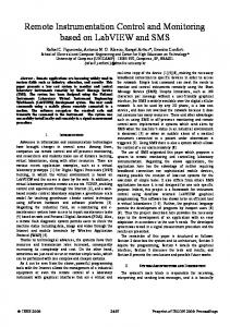
4.1. DIRECT STRESS σ When a force F acts directly on an area A as shown in figure 1, the resulting direct stress is the force per unit area and is given as σ = F/A. where F is the force normal to the area in Newtons A is the area in m2 and σ (sigma) is the direct stress in N/m2 or Pascals. Since 1 Pa is a small unit kPa , MPa and GPa are commonly used also. If the force pulls on the area so that the material is stretched then it is a tensile force and stress and this is positive. If the force pushes on the surface so that the material is compressed, then the force and stress is compressive and negative. 4.2.

DIRECT STRAIN ε Consider a piece of material of length L as shown in figure 1. The direct stress produces a change in length ∆L. The direct strain produced is ε (epsilon) defined as ε =∆L/L The units of change in length and original length must be the same and the strain has no units.

Figure 1 Strains are normally very small so often to indicate a strain of 10-6 we use the name micro strain and write it as µε. For example we would write a strain of 7 x 10-6 as 7µε. Tensile strain is positive and compressive strain is negative.

4.3. MODULUS OF ELASTICITY E Many materials are elastic up to a point. This means that if they are deformed in any way, they will spring back to their original shape and size when the force is released. It has been established that so long as the material remains elastic, the stress and strain are related by the simple formula E= σ /ε and E is called the MODULUS OF ELASTICITY. The units are the same as those of stress.

 D.J.Dunn

4

ELASTIC LIMIT A material is only elastic up to a certain point. If the elastic limit is exceeded, the material becomes permanently stretched. The stress-strain graph for some metals are shown below. The modulus of elasticity does not apply above the elastic limit. Strain gauges should not be stretched beyond the elastic limit of the strain gauge material which is approximately 3000µε.

Figure 2 A typical value for the elastic limit of strain gauges is 3000 µε.

WORKED EXAMPLE No.1 A metal bar which is part of a frame is 50 mm diameter and 300 mm long. It has a tensile force acting on it of 40 kN which tends to stretch it. The modulus of elasticity is 205 GPa. Calculate the stress and strain in the bar and the amount it stretches. SOLUTION F = 40 x 103 N. A = πD2/4 = π x 502/4 = 1963 mm2 σ = F/A = (40 x103 )/(1963 x 10-6) = 20.37 x 106 N/m2 =20.37 MPa E = σ /ε = 205 x 109 N/m2 ε = σ/E = (20.37 x 106)/(205 x 109) = 99.4 x 10-6 or 99.4 µε ε = ∆L/L ∆L= ε x L = 99.4 x 10-6 x 300 mm = 0.0298 mm

4.4. POISSONS' RATIO Consider a piece of material in 2 dimensions as shown in figure 2. The stress in the y direction is σy and there is no stress in the x direction. When it is stretched in the y direction, it causes the material to get thinner in all the other directions at right angles to it. This means that a negative strain is produced in the x direction. For elastic materials it is found that the applied strain (ε y) is always directly proportional to the induced strain (ε x) such that (ε x)/(ε y) = - ν where ν (Nu)is an elastic constant called Poissons' ratio. The strain produced in the x direction is ε x= - ν ε y Figure 3  D.J.Dunn

5

SELF ASSESSMENT EXERCISE No.2 1. A metal wire is 1 mm diameter and 1 m long. It is stretched by a force of 2 N. Calculate the change in diameter. E = 90 GPa and ν = 0.3 (Answer -8.5 x 10-6 mm). Explain what happens to the resistance of the wire. 2. Explain the significance of Poisson's ratio to the behaviour of strain gauges.

5.

RESISTIVITY

The resistance of a conductor increases with length L and decreases with cross sectional area A so we may say R is directly proportional to L and inversely proportional to A. R = Constant x L/A The constant is the resistivity of the material ρ hence R = ρL/A Ohms

SELF ASSESSMENT EXERCISE No.3 1. Calculate the resistance of a copper wire 5 m long and 0.3 mm diameter. The resistivity is 1.7 x 10-8 Ohm metre. (Answer 1.202 Ω) 2. Calculate the resistance of a nichrome wire 2 m long and 0.2 mm diameter given ρ = 108 x 10-8 (Answer 68.75 Ω)

6.

TEMPERATURE COEFFICIENT OF RESISTANCE

The resistance of conductors changes with temperature. This is a problem when strain gauge devices are used. Usually the resistance increases with temperature. The amount by which the resistance changes per degree per ohm of the original resistance is called the temperature coefficient of resistance and is denoted α. The units are Ohms per Ohm per degree. Let the resistance of a conductor be Ro at 0oC. Let the resistance be R1 at θ1 oC. The change in resistance = αθ1 Ro The new resistance is R1 = Ro + αθ1 Ro Let the resistance be R2 at θ2 oC. The change in resistance = αθ2 Ro The new resistance is R2 = Ro + αθ2 Ro If the temperature changes from θ1 to θ2 the resistance changes by ∆R = R2 - R1 = (Ro + αθ2 Ro ) - ( Ro + αθ1 Ro ) ∆R = Ro α ∆θ

SELF ASSESSMENT EXERCISE No.4 1. A resistor has a nominal resistance of 120 Ω at 0 oC. Calculate the resistance at 20oC. Calculate the change in resistance when the temperature drops by 5 degrees. α = 6 x 10 -3 Ω/Ω oC (Answers 134.4 Ω and - 3.6Ω)

 D.J.Dunn

6