INTEGER PROGRAMMING by V. Chandru2 & M. R. Rao3
March 1998
Please address all correspondence to: Dr. M. R. Rao Indian Institute ofManagement Bangalore Bannerghatta Road Bangalore 560 076 India Fax: (080) 6644050
*To appear as a chapter of the Handbook of Algorithms edited by M.J. Atallah, CRC Press (1998) 2
CS & Automation, Indian Institute of Science, Bangalore-560 012, India.
[email protected]
3
Indian Institute ofManagement Bangalore, Bangalore 560 076, India.
[email protected] Copies of the Working Papers may be obtained from the FPM & Research OflBce
INTEGER PROGRAMMING 4 VIJAY CHANDRU,
Indian Institute of Science, Bangalore 560 012, India.
M.R. RAO, Indian Institute of Management, Bangalore 560 076, India. JANUARY, 1998
Abstract Integer programming is an expressive framework for modeling and solving discrete optimization problems that arise in a variety of contexts in the engineering sciences. Integer programming representations work with implicit algebraic constraints (linear equations and inequalities on integer valued variables) to capture the feasible set of alternatives, and linear objective functions (to minimize or maximize over the feasible set) that specify the criterion for defining optimality. This algebraic approach permits certain natural extensions of the powerful methodologies of linear programming to be brought to bear on combinatorial optimization and on fundamental algorithmic questions in the geometry of numbers.
1
Introduction
In 1957 the Higgins lecturer of mathematics at Princeton, Ralph Gomory, announced that he would lecture on solving linear programs in integers. The immediate reaction he received was: "But that's impossible!". This was his first indication that others had thought about the problem [57]. Gomory went on to work on the foundations of the subject of integer programming as a scientist at IBM from 1959 until 1970 (when he took over as Director for Research). From cutting planes and the polyhedral combinatorics of corner polyhedra to group knapsack relaxations, the approaches that Gomory developed remain striking to researchers even today. There were other pioneers in integer programming who collectively played a similar role in developing techniques for linear programming in Boolean or 0-1 variables. These efforts were directed at combinatorial optimization problems such as Routing, Scheduling, Layout and Network Design. These are generic examples of combinatorial optimization problems that often arise in computer engineering and decision support. Unfortunately, almost all interesting generic classes of integer programming problems are AfVHard. The scale at which these problems arise in applications and the explosive exponential complex4
Readers unfamiliar with linear programming methodology are strongly encouraged to consult the chapter on linear
programming in this handbook. 1
ity of the search spaces preclude the use of simplistic enumeration and search techniques. Despite the worst-case intractability of integer programming, in practice we are able to solve many large problems and often enough with off-the-shelf software. Effective software for integer programming is usually problem specific and based on sophisticated algorithms that combine approximation methods with search schemes and that exploit mathematical (and not just syntactic) structure in the problem at hand. An abstract formulation of combinatorial optimization is {CO) min{/(J) : / € 1} where I is a collection of subsets of a finite ground set E = {ci,e2,.. .,c n } and / is a criterion (objective) function that maps 2E (the power set of E) to the reals. The most general form of an integer linear program is {MILP)
min {ex : Ax > b, Xj integer V j 6 J}
which seeks to minimize a linear function of the decision vector x subject to linear inequality constraints and the requirement that a subset of the decision variables are integer valued. This model captures many variants. If J = {1,2, . . . , n } , we say that the integer program is pure and mixed otherwise. Linear equations and bounds on the variables can be easily accomodated in the inequality constraints. Notice that by adding in inequalities of the form 0 < Xj < 1 for a j 6 J we have forced XJ to take value 0 or 1. It is such Boolean variables that help capture combinatorial optimization problems as special cases of (MILP). The next section contains preliminaries on linear inequalities, polyhedra, linear programming and an overview of the complexity of integer programming. These are the tools we will need to analyze and solve integer programs. Section 3, is the testimony on how integer programs model combinatorial optimization problems. In addition to working a number of examples of such integer programming formulations, we shall also review formal representation theories of (Boolean) mixed integer linear programs. With any mixed integer program we associate a linear programming relaxation obtained by simply ignoring the integrality restrictions on the variables. The point being, of course, that we have polynomial-time (and practical) algorithms for solving linear programs (see Chapter Editor: Please Insert the Number of the Chapter on Linear Programming of this handbook). Thus the linear programming relaxation of (MILP) is given by (LP)
min {ex : Ax > b}
The thesis underlying the integer linear programming approaches is that this linear programming relaxation retains enough of the structure of the combinatorial optimization problem, to be a
useful weak representation. In Section 4 we shall take a closer look at this thesis in that we shall encounter special structures for which this relaxation is "tight". For general integer programs, there are several alternate schemes for generating linear programming relaxations with varying qualities of approximation. A general technique for improving the quality of the linear programming relaxation is through the generation of valid inequalities or cutting planes. The computational art of integer programming rests on useful interplays between search methodologies and algebraic relaxations. The paradigms of Branch & Bound and Branch & Cut are the two enormously effective partial enumeration schemes that have evolved at this interface. These will be discussed in Section 5. It may be noted that all general purpose integer programming software available today uses one or both of these paradigms. A general principle, is that we often need to disaggregate integer formulations to obtain higher quality linear programming relaxations. To solve such huge linear programs we need specialized techniques of large-scale linear programming. These aspects are described in the chapter (Chapter -Editor: Please Fill In) on linear programming in this handbook. The reader should note that the focus in this chapter is on solving hard combinatorial optimization problems. We catalog several special structures in integer programs that lead to tight linear programming relaxations (Section 6) and hence to polynomial-time algorithms. These include structures such as network flows, matching and matroid optimization problems. Many hard problems actually have pieces of these nice structures embedded in them. Successful implementations of combinatorial optimization have always used insights from special structures to devise strategies for hard problems. The inherent complexity of integer linear programming has led to a long-standing research program in approximation methods for these problems. Linear programming relaxation and Lagrangean relaxation (Section 6) are two general approximation schemes that have been the real workhorses of computational practice. Primal-Dual strategies and Semi-Definite relaxations (Section 7) are two recent entrants that appear to be very promising. Pure integer programming with variables that take arbitrary integer values is a natural extension of diophantine equations in number theory. Such problems arise in the context of cryptography, dependence analysis in programs, the geometry of numbers and Presburgher arithmetic. Section 8 covers this aspect of integer programming. We conclude the chapter with brief comments on future prospects in combinatorial optimization from the algebraic modeling perspective.
2
Preliminaries
2.1
Polyhedral Preliminaries
Polyhedral combinatorics is the study of embeddings of combinatorial structures in Euclidean space and their algebraic representations. We will make extensive use of some standard terminology from polyhedral theory. Definitions of terms not given in the brief review below can be found in [95,124]. A (convex) polyhedron in 3Rn can be algebraically defined in two ways. The first and more straightforward definition is the implicit representation of a polyhedron in 3ftn as the solution set to a finite system of linear inequalities in n variables. A single linear inequality ax < OQ ; a ^ 0 defines a half-space of 9£n. Therefore geometrically a polyhedron is the intersection set of a finite number of half-spaces. A polytope is a bounded polyhedron. Every poly tope is the convex closure of a finite set of points. Given a set of points whose convex combinations generate a polytope we have an explicit or parametric algebraic representation of it. A polyhedral cone is the solution set of a system of homogeneous linear inequalities. Every (polyhedral) cone is the conical or positive closure of a finite set of vectors. These generators of the cone provide a parametric representation of the cone. And finally a polyhedron can be alternately defined as the Minkowski sum of a polytope and a cone. Moving from one representation of any of these polyhedral objects to another defines the essence of the computational burden of polyhedral combinatorics. This is particularly true if we are interested in "minimal" representations. A set of points x 1 , . . . , x m is affinely independent if the unique solution of YZLi ^ X * = 0, Y^Li ^* == 0 is Aj = 0 for i = 1 , . . . , m . Note that the maximum number of affinely independent points in 3ftn is n-f 1. A polyhedron P is of dimension A:, dim P = fc, if the maximum number of affinely independent points in P is k + 1. A polyhedron P C 3ftn of dimension n is called full-dimensional. An inequality a x < a 0 is called valid for a polyhedron P if it is satisfied by all x in P. It is called supporting if in addition there is an x in P that satisfies ax = OQ. A face of the polyhedron is the set of all x in P that also satisfy a valid inequality as an equality. In general, many valid inequalities might represent the same face. Faces other than P itself are called proper. A facet of P is a maximal nonempty and proper face. A facet is then a face of P with a dimension of d i m P — 1. A face of dimension zero, i.e. a point v in P that is a face by itself, is called an extreme point of P. The extreme points are the elements of P that cannot be expressed as a strict convex combination of two distinct points in P. For a full-dimensional polyhedron, the valid inequality representing a facet is unique up to multiplication by a positive scalar, and facet-inducing inequalities give a minimal implicit representation of the polyhedron. Extreme points, on the other hand, give rise to minimal parametric representations of polytopes.
The two fundamental problems of linear programming (which are polynomially equivalent) are: • Solvability This is the problem of checking if a system of linear constraints on real (rational) variables is solvable or not. Geometrically, we have to check if a polyhedron, defined by such constraints, is nonempty. • Optimization This is the problem (LP) of optimizing a linear objective function over a polyhedron described by a system of linear constraints. Building on polarity in cones and polyhedra, duality in linear programming is a fundamental concept which is related to both the complexity of linear programming and to the design of algorithms for solvability and optimization. Here we will state the main duality results for optimization. If we take the primal linear program to be (P) min {ex : Ax > b} there is an associated dual linear program (D) max {b T y : ATy = c T , y > 0} and the two problems satisfy 1. For any x and y feasible in (P) and (D) (i.e. they satisfy the respective constraints), we have ex > b T y (weak duality). Consequently, (P) has a finite optimal solution if and only if (D) does. 2. x* and y* are a pair of optimal solutions for (P) and (D) respectively, if and only if x* and y* are feasible in (P) and (D) (i.e. they satisfy the respective constraints) and ex* = b T y* (strong duality). 3. x* and y* are a pair of optimal solutions for (P) and (D) respectively, if and only if x* and y* are feasible in (P) and (D) (i.e. they satisfy the respective constraints) and (Ax* — b) T y* = 0 (complementary slackness). The strong duality condition gives us a good stopping criterion for optimization algorithms. The complementary slackness condition, on the other hand gives us a constructive tool for moving from dual to primal solutions and vice-versa. The weak duality condition gives us a technique for obtaining lower bounds for minimization problems and upper bomnds for maximization problems. Note that the properties above have been stated for linear programs in a particular form. The reader should be able to check, that if for example the primal is of the form (P7) min^cx : Ax =s b, x > 0}
then the corresponding dual will have the form (D')
max{bTy:ATy 0. The linear programming relaxation associated with (P8) is obtained by replacing constraints yi = 0 or 1, and xt*7- = 0 or 1 by non-negativity contraints on xtj and yt-. The upper bound constraints on yt- are not required provided /» > 0, i = 1,2, ..,m. The upper bound constraints on x»j are not required in view of constraints
YALI
x
ij = !•
Remark: It is frequently possible to formulate the same combinatorial problem as two or more different ILPs. Suppose we have two ILP formulations (Fl) and (F2) of the given combinatorial problem with both (Fl) and (F2) being minimizing problems. Formulation (Fl) is said to be stronger than (F2) if (LP1), the the linear programming relaxation of (Fl), always has an optimal objective function value which is greater than or equal to the optimal objective function value of (LP2) which is the linear programming relaxation of (F2). 35
It is possible to reduce the number of constraints in (P8) by replacing the constraints Xij - yi < 0 by an aggregate: n
Y^ij
-nyi b , x 6 l C » n }
Implicit in this representation is the assumption that the explicit constraints (Ax > b) are "small" in number. For convenience let us also assume that that X can be replaced by a finite list {x^x 2 , ...x T }. The following definitions are with respect to (P) • Lagrangean
£(u,x) = n(Ax - b) + ex where u are the Lagrange multipliers.
• tt Lagrangean Subprobiem
nun x€ x{£(u,x)}
36
• Lagrangean-Dual Function • Lagrangean-Dual Problem
£(u) = min x€ x{£(u,x)} (D)
d = max u > 0 {£(u)}
It is easily shown that (D) satisfies a weak duality relationship with respect to (P), i.e., z > d. The discreteness of X also implies that £(u) is a piece-wise linear and concave function (see Shapiro 115]). In practice, the constraints X are chosen such that the evaluation of the Lagrangean Dual "unction £(u) is easily made. An Example:
Traveling Salesman Problem (TSP)
For an undirected graph G, with costs on each edge, the TSP is to find a minimum cost set H of edges of G such that it forms a Hamiltonian cycle of the graph. H is a Hamiltonian cycle of G if it is a simple cycle that spans all the vertices of G. Alternately H must satisfy: 1. exactly two edges of H are adjacent to each node, and 2. H forms a connected, spanning subgraph of G. Held and Karp [63] used these observations to formulate a Lagrangean relaxation approach for TSP, that relaxes the degree constraints (1). Notice that the resulting subproblems are minimum spanning tree problems which can be easily solved. The most commonly used general method of finding the optimal multipliers in Lagrangean relaxation is subgradient optimization (cf. Held et al. [62]). Subgradient optimization is the nondifferentiable counterpart of steepest descent methods. Given a dual vector \ik, the iterative rule for creating a sequence of solutions is given by:
where tjt is an appropriately chosen step size, and 7(11*) is a subgradient of the dual function C at \ik. Such a subgradient is easily generated by
where x* is an optimal solution of min xG jr{^(u^x)}. Subgradient optimization has proven effective in practice for a variety of problems. It is possible to choose the step sizes { 0 and integer}
Since A and b are integer matrices, the fractional parts of elements of B~lN and B~lb are of the form (3^5) where k G {0, l,...,|det#| - 1}. The congruences in (ILPG) are equivalent to working 38
in a product of cyclic groups. The structure of the product group is revealed by the Hermite Normal Form of B (see Section 2.2). Hence Hence (ILPG)
is referred to as a group (knapsack) problem and
is solved by a dynamic programming algorithm [58]. 6.4
Semi-Definite Relaxation
Semi-definite programs are linear optimization problems defined over a cone of positive semi-definite matrices. These are models that generalize linear programs and are specializations of convex programming models. There are theoretical and "practical" algorithms for solving semi-definite programs in polynomial time [3]. Lovasz and Schrijver [91] suggest a general relaxation strategy for 0 — 1 integer programming problems that obtains semi-definite relaxations. The first step is to consider a homogenized version of a 0 — 1 integer program (solvability version). JF7 = { x e » n + 1 : A x > 0 , x o = 1, Xi£ {0,l}fori = 1,2, ••• > n} The problem is to check if Fj is non-empty. Note that any 0 — 1 integer program can be put in this form by absorbing a general right-hand-side 6 as the negative of xo column of A. Now a linear programming relaxation of this integer program is given by: A x > 0, x o = l, 0 < x, < x 0 for t = 1,2, • •-,n} Next, we define two polyhedral cones. K = { x e £ n + 1 : A x > 0 , 0 < x t < x 0 f o r i = 0,l, — , n } /C/ = Cone generated by 0 - 1 vectors in P / Lovasz and Schrijver [91] show how we might construct a family of convex cones {C} such that £ / C C C K for each C. (i) Partition the cone constraints of K into 2\ = {A\x > 0} and T2 = {A2X > 0}, with the constraints {0 < xt- < xo for i = 0 , 1 , • • -,n} repeated in both (the overlap can be larger). (ii) Multiply each constraint in T\ with each constraint in T2 to obtain a quadratic homogeneous constraint. (iii) Replace each occurance of a quadratic term X{Xj by a new variable -X"^-. The quadratic constraints are now linear homogeneous constraints in X{j. (iv) Add the requirement that the ( n + l ) x {n+l) matrix X is symmetric and positive semi-definite, (v) Add the constraints Xot = Xa for i = 1,2, • • •, n. 39
The system of constraints on the XtJ- constructed in steps (iii), (iv) and (v) above define a cone M+{Ti,T2) parametrized by the partition TUT2. We finally project the cone M+(TUT2) to $ln+l as follows. C+{TUT2) = Diagonals of matrices in Af + (Ti,r 2 ) These resulting cones {C+(Ti,T2)} satisfy Id C C + (T lf r 2 ) C K where the Xu in C+(Ti,T2) are interpreted as the original xt- in K and /C/. One semi-definite relaxation of the 0 — 1 integer program Fj is just C+(Ti,T2) along with the normalizing constraint Xoo = so = 1- For optimization versions of integer programming, we simply carry over the objective function. An amazing result obtained by Lovasz and Schrijver [91] is that this relaxation when applied to the vertex packing polytope (see Section 3.4) is atleast as good as one obtained by adding "clique, odd hole, odd antihole and odd wheel" valid inequalities (see [61] for the definitions) to the linear programming relaxation of the set packing formulation. This illustrates the power of this approach to reveal structure and yet obtain a tractable relaxation. In particular, it also implies a polynomial-time algorithm for the vertex packing problem on perfect graphs (cf. [61]). Another remarkable success that semi-definite relaxations have registered is the recent result on finding an approximately maximum weight edge cutset of a graph. This result of Goemans and Williamson [55] will be described in the next section. While the jury is still out on the efficacy of semi-definite relaxation as a general strategy for integer programming, there is little doubt that it provides an exciting new weapon in the arsenal of integer programming methodologies.
7
Approximation with Performance Guarantees
The relaxation techniques7 we encountered in the previous section are designed with the intent of obtaining a "good" lower (upper) bound on the optimum objective value for a minimization (maximization) problem. If in addition, we are able to construct a "good" feasible solution using a heuristic (possibly based on a relaxation technique) we can use the bound to quantify the suboptimality of the incumbent and hence the "quality of the approximation". In the past few years, there has been significant progress in our understanding of performance guarantees for approximation of J\fP-Hard combinatorial optimization problems (cf.[117]). A papproximate algorithm for an optimization problem is an approximation algorithm that delivers a feasible solution with objective value within a factor of p of optimal (think of minimization problems and p > 1). For some combinatorial optimization problems, it is possible to efficiently find solutions that are arbitrarily close to optimal even though finding the true optimal is hard. If this were true 40
of most of the problems of interest we would be in good shape. However, the recent results of Arora et al. [5] indicate exactly the opposite conclusion. A PTAS or polynomial-time approximation scheme for an optimization problem is a family of algorithms Ap, such that for each p > 1, Ap is a polynomial-time /^approximate algorithm. Despite concentrated effort spanning about two decades, the situation in the early 90's was that for many combinatorial optimization problems, we had no PTAS and no evidence to suggest the non-existence of such schemes either. This led Papadimitriou and Yannakakis [104] to define a new complexity class (using reductions that preserve approximate solutions) called MAXSNP and they identified several complete languages in this class. The work of Arora et al. completed this agenda by showing that, assuming V ^ AfV, there is no PTAS for a MAXSNP-complete problem. An implication of these theoretical developments is that for most combinatorial optimization problems, we have to be quite satisfied with performance guarantee factors p > 1 that are of some small fixed value. (There are problems, like the general traveling salesman problem, for which there are no /^approximate algorithms for any finite value of p - of course assuming V ^ AfV). Thus one avenue of research is to go problem by problem and knock p down to its smallest possible value. A different approach would be to look for other notions of "good approximations" based on probabilistic guarantees or empirical validation. A good example of the benefit to be gained from randomization is the problem of computing the volume of a convex body. Dyer and Frieze [37]have shown that this problem is ^'P-hard. Barany and Furedic[8] provide evidence that no polynomialtime deterministic approximation method with relative error less than (cn)%, where c is a constant, is likely to exist. However, Dyer et al. [38] have designed a fully-polynomial randomized approximation scheme (FPRAS) for this problem. The FPRAS of Dyer et al. citeDFK uses techniques from integer programming and the geometry of numbers (see Section 8). L P R E L A X A T I O N AND R O U N D I N G
Consider the well known problem of finding the smallest weight vertex cover in a graph (see Section 3.1). So we are given a graph G(V, E) and a nonnegative weight 10(11) for each vertex v € V. We want to find the smallest total weight subset of vertices 5 such that each edge of G has at least one end in 5 (This problem is known to be MAXSNP-Hard). An integer programming formulation of this problem is given by w(v)x(v):x{u) + x(v) > 1, V(u,v) € E, x{v) €
{0,l}VveV}
vev To obtain the linear programming relaxation we substitute the x(v) 6 {0,1} constraint with x(v)>0
for each v e V. Let x* denote an optimal solution to this relaxation. Now let us round the
fractional parts of x* in the usual way, that is, values of 0.5 and up are rounded to 1 and smaller 41
values to 0. Let x be the 0-1 solution obtained. First note that x(v) < 2xm(v) for each v £ V. Also, for each (u,v) 6 E, since x*(u) + x*(v) > 1, at least one of x(u) and x(v) must be set to 1. Hence x is the incidence vector of a vertex cover of G whose total weight is within twice the total weight of the linear programming relaxation (which is a lower bound on the weight of the optimal vertex cover). Thus we have a 2-approximate algorithm for this problem which solves a linear programming relaxation and uses rounding to obtain a feasible solution. The deterministic rounding of the fractional solution worked quite well for the vertex cover problem. One gets a lot more power from this approach by adding in randomization to the rounding step. Raghavan and Thompson [108] proposed the following obvious randomized rounding scheme. Given a 0 - 1 integer program, solve its linear programming relaxation to obtain an optimal x*. Treat the $j* € [0,1] as probabilities , i.e. let Probability{zj = 1}= ZJ*, to randomly round the fractional solution to a 0 — 1 solution. Using Chernoff bounds on the tails of the Binomial distribution, they were able to show, for specific problems, that with high probability, this scheme produces integer solutions which are close to optimal. In certain problems, this rounding method may not always produce a feasible solution. In such cases, the expected values have to be computed as conditioned on feasible solutions produced by rounding. More complex (non-linear) randomized rounding schemes have been recently studied and have been found to be extremely effective. We will see an example of non-linear rounding in the context of semi-definite relaxations of the max-cut problem below. PRIMAL DUAL APPROXIMATION
The linear programming relaxation of the vertex cover problem, we saw above, is given by (Pvc)
min{^iy(v)x(t;):a;(u) + x(v)> 1, V(u,v) € E, vev
x{v) > 0Vt;€ V}
and its dual is {Dye)
max{ £
y ( u , v) :
JT
y(u, v) < w{v), Vv € V,
y{uy v)>0
V(ti, v) 6 E}
The primal-dual approximation approach would first obtain an optimal solution y* to the dual problem (Dvc)- Let V CV denote the set of vertices for which the dual constraints are tight, i.e.,
V={veV:
J2
y*(u,v) = w(v)}
u\{utv)eE
The approximate vertex cover is taken to be V. It follows from complementary slackness that V is a vertex cover. Using the fact that each edge (it, v) is in the star of at most two vertices (u and v), it also follows that V is a 2-approximate solution to the minimum weight vertex cover problem. In general, the primal-dual approximation strategy is to use a dual solution, to the linear programming relaxation, along with complementary slackness conditions as a heuristic to generate an 42.
integer (primal) feasible solution which for many problems turns out to be a good approximation of the optimal solution to the original integer program. It is a remarkable property of the vertex covering (and packing) problem that all extreme points of the linear programming relaxation have values 0, \ or 1 [94], It follows that the deterministic rounding of the linear programming solution to (Pvc) constructs exactly the same approximate vertex cover as the primal-dual scheme described above. However, this is not true in general. SEMI-DEFINITE RELAXATION AND ROUNDING
The idea of using semi-definite programming to approximately solve combinatorial optimization problems appears to have originated in the work of Lovasz [90] on the Shannon capacity of graphs. Grotschel, Lovasz and Schrijver [61] later used the same technique to compute a maximum stable set of vertices in perfect graphs via the ellipsoid method. As we saw in Section 7.4, Lovasz and Schrijver [91] have devised a general technique of semi-definite relaxations for general 0 — 1 integer linear programs. We will present a lovely application of this methodology to approximate the the maximum weight cut of a graph (the maximum sum of weights of edges connecting across all strict partitions of the vertex set). This application of semi-definite relaxation for approximating MAXCUT is due to Goemans and Williamson [55]. We begin with a quadratic Boolean formulation of MAXCUT max{|
£
w{u,v){l-x(u)x{v)):
x(v) € {-1,1} V v 6 V}
(
where G(V, E) is the graph and tt/(ti,v) is the non-negative weight on edge (it, v). Any {—1,1} vector of x values provides a bipartition of the vertex set of G. The expression (1 - x(u)x(v)) evaluates to 0 if u and v are on the same side of the bipartition and 2 otherwise. Thus, the optimization problem does indeed represent exactly the MAXCUT problem. Next we reformulate the problem in the following way. • We square the number of variables by allowing each x(v) to denote an n-vector of variables (where n is the number of vertices of the graph). • The quadratic term x(u)x(v) is replaced by x(u) -x(v) which is the inner product of the vectors. • Instead of the {—1,1} restriction on the x(v), we use the Euclidean normalization ||x(v)|| — 1 on the x(v). So we now have a problem £
I»(TI,V)(1-X(U).X(TO):
43
||X(V)|| = 1 V v € V}
which is a relaxation of the MAXCUT problem (note that if we force only the first component of the x(t;)'s to have nonzero value, we would just have the old formulation as a special case). The final step is in noting that this reformulation is nothing but a semi-definite program. To see this we introduce n x n Gram matrix Y of the unit vectors x(v). So Y = XTX where X = (x(v) : v 6 V). So the relaxation of MAXCUT can now be stated as a semi-definite program. ^
w{u,v){l-Y(UtV)):
Y y 0, Y(t,jtl) = 1 V v G V}
Note that we are able to solve such semi-definite programs to an additive error e in time polynomial in the input length and log ~ using either the Ellipsoid method or Interior Point methods (see [3] and Chapters Editor: Please cross reference chapters on Linear programming, Approximation and Nonlinear Programming of this handbook). Let x* denote the near optimal solution to the semi-definite programming relaxation of MAXCUT (convince yourself that x* can be reconstructed from an optimal Y* solution). Now we encounter the final trick of Goemans and Williamson. The approximate maximum weight cut is extracted from x* by randomized rounding. We simply pick a random hyperplane H passing through the origin. All the v € V lying to one side of H get assigned to one side of the cut and the rest to the other. Goemans and Williamson observed the following inequality. Lemma 7.1 For xi and X2, two random n-vectors of unit norm, let x(l) and z(2) be ±1 values with opposing sign if H separates the two vectors and with same signs otherwise. Then E(l - XiTX2) < 1.1393- E(l - x(l)x(2)) where E denotes the expected value. By linearity of expectation, the lemma implies that the expected value of the cut produced by the rounding is at least 0.878 times the expected value of the semi-definite program. Using standard conditional probability techniques for derandomizing, Goemans and Williamson show that a deterministic polynomial-time approximation algorithm with the same margin of approximation can be realized. Hence we have a cut with value at least 0.878 of the maximum value.
8
Geometry of Numbers and Integer Programming
Given an integer program with a fixed number of variables (A:) we seek a polynomial-time algorithm for solving them. Note that the complexity is allowed to be exponential in k, which is independent of the input length. Clearly if the integer program has all (0,1) integer variables this is a trivial task, since complete enumeration works. However if we are given an "unbounded" integer program to begin with, the problem is no longer trivial.
44
8.1
Lattices, Short Vectors and Reduced Bases
Euclidean lattices are a simple generalization of the regular integer lattice Zn. A (point) Lattice is specified by {bx, • • •, b n } a basis (where b; are linearly independent n - dimensional rational vectors). The Lattice L is given by : L = {x: x = t=i
B = (bi : b2: • • •: b n ) a basis matrix of L Theorem 8.1 \detB\ is an invariant property of the lattice L (ie for every basis matrix Bi of L we have invariant d(L) = \detBi\). Note that d(L) = njLjjbil where |b»|denotes the Euclidean Length of b* if and only if the basis vectors {b»} are mutually orthogonal. A "sufficiently orthogonal" basis B (called a reduced basis) is one that satisfies a weaker relation d(L) < Cn IIJLJbil where Cn is a constant that depends only on n One important use (from our perspective) of a reduced basis is that one of the basis vectors has to be "short". Note that there is sunstantive evidence that finding the shortest lattice vector is jVP-Hard [61]. Minkowski proved that in every lattice L there exists a vector of length no larger than Cy/ny/d(L) (with c no larger than 0.32). This follows from the celebrated MinkowskFs Convex Body Theorem which forms the centerpiece of the geometry of numbers [19]. Theorem 8.2 Minkowski's Convex Body Theorem: If K C 3fJn is a convex body that is centrally symmetric with respect to the origin, and L C 3ftn is is a lattice such that vol(K) > 2nd(L) then K contains a lattice point different from the origin. However, no one has been successful thus far in designing an efficient algorithm (polynomial-time) for constructing the short lattice vector guaranteed by Minkowski. This is where the concept of a reduced basis comes to the rescue. We are able to construct a reduced basis in polynomial time and extract a short vector from it. To illustrate the concepts we will now discuss an algorithm due to Gauss (cf. [6]) that proves the theorem for the special case of planar lattices (n = 2). It is called the 60° Algorithm because it produces a reduced basis {bi,b 2 } such that the acute angle between the two basis vectors is at least 60°.
45
Procedure: 60° Algorithm Input:
Basis vectors bi and b2 with \b\\ > 11>2j.
Output:
A reduced basis {bi,b2} with at least 60° angle between the basis
vectors.
0. repeat u n t i l jl>iJ < |l>2| 1. swap bi and 2. b 2 t- (b2 - mbi) and m =
|
6 Z.
Here [a] denotes the integer nearest to a. 3. end
II Y4L
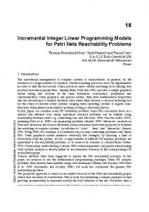
Figure 4: A Reduced Basis REMARKS:
(i) In each iteration the projection of (b2 — mbi) onto the direction of bi is of length atmost |bi|/2. (ii) When the algorithm stops b2 must lie in one of the shaded areas at the top or at the bottom of Figure 4 (since Jb^l > |bi| and since the projection of b 2 must fall within the two vertical lines about bi). (iii) The length of bx strictly decreases in each iteration. Hence the algorithm is finite. That it is polynomial time takes a little more argument [82]. 46
(iv) The short vector b x produced by the algorithm satisfies \bx\ < (1.075)(d(L))2). The only known polynomial-time algorithm for constructing a reduced basis in an arbitrary dimensional lattice [86] is not much more complicated than the 60° algorithm. However, the proof of polynomiality is quite technical (see [6] for an exposition). 8.2
Lattice Points in a Triangle
Consider a triangle T in the Euclidean plane defined by the inequalities
+ ^32^2 ^ ^3
The problem is to check if there is a lattice point ( x i , ^ ) € Z2 satisfying the three inequalities. The reader should verify that checking all possible lattice points within some bounding box of T leads to an exponential algorithm for skinny and long triangles. There are many ways of realizing a polynomial-time search algorithm [73,46] for two-variable integer programs. Following Lenstra [88] we describe one that is a specialization of his [87] powerful algorithm for integer programming (searching for a lattice point in a polyhedron). First we use a nonsingular linear,transform r that makes T equilateral (round). The transform sends the integer lattice Z2 to a generic two-dimensional lattice L. Next we construct a reduced basis {bi,b2} for L using the 60° algorithm. Let /?i denote the length of the short vector b i . If I denotes the length of a side of the equilateral triangle r(T) we can conclude that T is guaranteed to contain a lattice point if J^ > \ / 6 . Else I < y/EP\ and we can argue that just a few (no more than 3) of the lattice lines {Affine Hull{bi} + kb2}kez can intersect T. We recurse to the lower dimensional segments (lattice lines intersecting with T) and search each segment for a lattice point. Hence this scheme provides a simple polynomial-time algorithm for searching for a lattice point in a triangle. 8.3
Lattice Points in Polyhedra
In 1979, H.W. Lenstra Jr. announced that he had a polynomial-time algorithm for integer programming problems with a fixed number of variables. The final published version [87] of his algorithm resembles the procedure described above for the case of a triangle and a planar lattice. As we have noted before, integer programming is equivalent to searching a polyhedron specified by a system of linear inequalities for an integer lattice point. Lenstra's algorithm then proceeds as follows.
47
• First "round" the polyhedron using a linear transformation. This step can be executed in polynomial time (even for varying n) using any polynomial-time algorithm for linear programming. • Find a reduced basis of the transformed lattice. This again can be done in polynomial time even for varying n. • Use the reduced basis to conclude that a lattice point must lie inside or recurse to several lower dimensional integer programs by slicing up the polyhedron using a "long" vector of the basis to ensure that the number of slices depends only on n. A slightly different approach based, on Minkowski's convex body theorem was designed by Kannan [74] to obtain an 0{nTL algorithm for integer programming (where L is the length of the input). The following two theorems are straightforward consequences of these polynomial-time algorithms for integer programming with a fixed number of variables. Theorem 8,3 (Fixed Number of Constraints) Checking the solvability of Ax < b; x 6 Zn where A is (m x n) is solvable in polynomial time if m is held fixed. Theorem 8.4 (Mixed Integer Programming) Checking the solvability of Ax < b; Xj 6 Z for j = 1, • • •, A;; Xj £ 3£ for j = k + 1, • • •, n where A is (m x n) is solvable in polynomial time i/min{m,fc} is held fixed. A related but more difficult question is that of counting the number of feasible solutions to an integer program or equivalently counting the number of lattice points in a polytope. Building on results described above, Barvinok [9] was able to show the following. Theorem 8.5 (Counting Lattice Points) Counting the size of the set {x e Zk : Ax < b} is solvable in polynomial time if k is held fixed. 8.4
An Application in Cryptography
In 1982, Adi Shamir [114] pointed out that Lenstra's algorithm could be used to devise a polynomialtime algorithm for cracking the basic Merkle-Hellman Cryptosystem (a knapsack based public-key cryptosystem). In such a rryptosystem the message to be sent is a (0-1) string x € {0,l} n . The 48
message is sent as an instance of the (0,1) knapsack problem which asks for an x € {0, l } n satisfying ]£?=i a » x t = ao- The knapsack problem is an .ATP-hard optimization problem (we saw in Section 3.4 that any integer program can be aggregated to a knapsack). However, if {a^} form a superincreasing sequence i.e., a» > £ j = \ CLJ Vi the knapsack problem can be solved in time O(n) by a simple algorithm:
Procedure:
0.
Best-Fit
JMl
1. If Oi< ao, Xi < - 1, CLQ
YA=I ai an( * U is relatively prime to M (ie gcd(U, M) = 1). Instead of {a»}, the sequence {a^ = I7a;(mod M)} 1=1|2t ..., n is published and do = Uao(mod M) is transmitted. Any receiver who "knows" U and M can easily reconvert {hi} to {a»-} and apply the best fit algorithm to obtain the message x. To find a^ given d^, U and M, he runs the Euclidean Algorithm on (U,M) to obtain 1 = PU + QM. Hence P is the inverse multiplier of U since PU = 1 (mod Af). Using the identity di = Phi (mod M) Vi = 0,1, • - •, n, the intended receiver can now use the best fit method to decode the message. An eavesdropper knows only the {d^} and is therefore supposedly unable to decrypt the message. The objective of Shamir's cryptanalyst (code breaker) is to find a P and in M (Positive integer) such that : O{ = Phi mod M Vi = 0 , 1 , • • •, n (*)
{dt};=if...tn is a super increasing sequence.
It can be shown that for all pairs {P,M) such that {P/M) is "sufficiently"close to (P/M) will satisfy (*). Using standard techniques from diophantine approximation it would be possible to guess P and M from the estimate (P/M).
However, the first problem is to get the estimate of (P/M).
This is where integer programming helps.
49
Since a,i = Pai (mod M) for i = 1,2, • • •, n we have a^Pdi — yiM for some integers yi, 1/2 > • * * > Vn Dividing by~a.{Mwe have (( TT^^TT) ) == — — -- zr zr for z = 1,2, • - . , n . For small t ( l , 2 , 3 , •••,*) the LHS \CLiM J
M
CLi
^ 0 since £?=i a{ < M and the {a;} t=1| ... >n are super-increasing. Thus {yi/ai), (2/2/^2), ••', (yt/a>t) are "close to" (P/M) and hence to each other. Therefore a natural approach to estimating (P/M) would be to solve the integer program:
Find 1/1,
,yt € 2 such that :
i for i = o
€i