Integral LOS Control for Path Following of Underactuated ... - CiteSeerX

Proceedings of the 47th IEEE Conference on Decision and Control Cancun, Mexico, Dec. 9-11, 2008

ThB16.5

Integral LOS Control for Path Following of Underactuated Marine Surface Vessels in the Presence of Constant Ocean Currents Even Børhaug, A. Pavlov and Kristin Y. Pettersen Norwegian University of Science and Technology, NO-7491 Trondheim, Norway.

paper, however, we study the particular problem for marine surface vessels. In particular, we pair the proposed guidance law with a set of adaptive tracking controllers and prove that the proposed control approach gives global asymptotic path following in the presence of constant, irrotational ocean currents. We study the problem both at the kinematic and dynamic level and provide explicit bounds on the parameters of the proposed guidance law. This paper is organized as follows. In Section II, we present the system model and state the control problem to be solved. In Section III we review traditional LOS guidance and in Section IV we present the controllers that solve the control problem stated in Section II. In Section V we formulate the I. I NTRODUCTION main technical result of the paper and present the proof of this In this paper, we consider the problem of path following of result in Section VI. Conclusions are given in Section VII. underactuated marine surface vessels in the presence of ocean II. S YSTEM M ODEL AND C ONTROL O BJECTIVE currents. In particular, we consider the problem of following In this section, we present the mathematical model of a straight-line path with a desired speed in the presence of the class of vessels considered in this paper. Moreover, constant, irrotational ocean currents. we introduce notation to be used throughout the paper and Path following control methods based on the Line-of-Sight formulate the control problem to be solved. (LOS) guidance principle are widely used (see e.g. [1–5]) and LOS guidance has some nice properties. In particular, LOS A. Vessel Model guidance is designed to mimic the actions of a helmsman, We consider the class of marine surface vessel that can be which will typically steer the vessel towards a point lying described by the 3-DOF model ([6]): a constant distance, called the look-ahead distance, ahead x˙ = u cos ψ − v sin ψ (1a) of the vessel, along the desired path. LOS guidance is simple, intuitive and easy to tune and gives, in the case y˙ = u sin ψ + v cos ψ (1b) of no environmental disturbances, nice path convergence ˙ ψ = r, (1c) properties. However, path following control approaches based M RB ν˙ + C RB (ν)ν = −M A ν˙ r − C A (ν r )ν r on traditional LOS guidance are susceptible to environmental Abstract— In this paper, we consider the development of a control strategy for path following of underactuated marine surface vessels in the presence of ocean currents. The proposed control strategy is based on a modified Line-of-Sight (LOS) guidance law with integral action and a pair of adaptive feedback controllers. Traditional LOS guidance has several nice properties and is widely used in practice for path following of marine vehicles. However, it has the drawback of being susceptible to environmental disturbances. In this work, we propose a modified LOS guidance law with integral action for counteracting environmental disturbances. Paired with a set of adaptive feedback controllers, we show that this approach guarantees global asymptotic path following of straight-line paths in the presence constant and irrotational ocean currents.

disturbances such as ocean currents, waves and wind. In particular, path deviation and convergence problems will occur if the vessel is affected by environmental disturbances. Moreover, this drawback cannot be fixed by simply adding integral action to the heading controller, i.e. by using a PID controller, since the source of the problem originates from the heading reference generator, that is, the LOS guidance law itself. The main contribution of this paper is a new guidance law with integral action. The proposed guidance law is based on the LOS guidance principle, but includes integral action to counteract environmental disturbances. The new guidance law overcomes the above mentioned drawbacks of traditional LOS guidance, while preserving the intuition and the simplicity of traditional LOS guidance. For this reason, the guidance law presented in this paper is applicable to a wide range of systems and not just marine surface vessels. In this

978-1-4244-3124-3/08/$25.00 ©2008 IEEE

− Dν r + Bf .

(1d)

Here, (x, y, ψ) is the position and orientation of the vessel with respect to an inertial reference frame i and ν  [u, v, r]T is a vector of body-fixed velocities, where u is the surge velocity, v is the sway velocity and r is the yaw angular velocity, respectively. Moreover, ν r  ν − ν c is the relative velocity of the vehicle, where ν c = RT (ψ)v c  [uc , vc , 0]T is the ocean current velocity expressed in body frame coordinates and v c  [Vx , Vy , 0]T is the ocean current velocity expressed in inertial coordinates. The inertial ocean current v c is assumed to be constant and irrotational, i.e. v˙ c = 0. This gives that  d  T (2) R (ψ)v c = [rvc , −ruc , 0]T . ν˙ c = dt The vector f ∈ R2 is the control input vector. Notice that the model (1d) is underactuated, since the dimension

4984

47th IEEE CDC, Cancun, Mexico, Dec. 9-11, 2008

ThB16.5

of the control input vector f is one less than the system dimension. Furthermore, the matrix M RB = M TRB > 0 is the rigid-body mass and inertia matrix, C RB is the rigidbody Coriolis and centripetal matrix, M A = M TA > 0 is the hydrodynamic added mass matrix, C A is the added mass Coriolis and centripetal matrix, D is the hydrodynamic damping matrix and B ∈ R3×2 is the actuator configuration matrix. The system matrices M RB , M A , D and B are assumed to have the following structure: ⎤ ⎡ x 0 0 m11 mx22 mx23 ⎦ , x ∈ {RB, A}, (3a) Mx  ⎣ 0 0 mx23 mx33 ⎤ ⎡ ⎤ ⎡ 0 b11 0 d11 0 D  ⎣ 0 d22 d23 ⎦ , B  ⎣ 0 b22 ⎦ , (3b) 0 d32 d33 0 b32

we instead make the assumption that the ocean current is constant in the inertial frame, i.e. that v˙ c = 0, which is a more natural assumption. B. Control Objective

The goal of this paper is to design a control system for the vessel, which dynamics are described by (6), such that starting from any location, the vessel converges to and follows a given straight-line path P with a desired constant speed Ud > 0. This statement should hold also in the presence of an unknown, constant and irrotational inertial ocean currents v c = [Vx , Vy , 0]T . To this end, we place the inertial coordinate system i with the x-axis along the desired path. With this choice, the desired path is given by P  {(x, y) ∈ R2 : y = 0} and the y-position of the vessel can be seen as the cross-track error, i.e. the minimum distance from the vessel to the desired path.With this notation, the T where M x = M x > 0. To obtain the particular structure of control objective can be formalized as the system matrices given in (3), we have assumed that the lim y(t) = 0, (7) t→∞ vessel is port-starboard symmetric (most vessels are) and that (8) lim ψ(t) = ψss , ψss ∈ (−π/2, π/2) , the body-fixed coordinate system, which we can freely choose t→∞ the position and orientation of, is located along the centerline (9) lim U (t) = Ud . t→∞ of the vessel (see [6]). With the above given structure for  M RB and M A , the Coriolis and centripetal matrices C RB Here, U  u(t)2 + v(t)2 is the total speed of the vessel and C A can be parameterized as (see [6]): and ψss is a constant. ⎡ ⎤ Remark: Note that we do not require that ψ(t) → 0 as 0 0 c13 (z2 , z3 ) ⎣ ⎦ t → ∞, but rather that ψ converges to a constant value ψss , 0 0 c23 (z1 ) C x (z)  , (4) where ψss ∈ (−π/2, π/2). In the presence of currents, the 0 −c13 (z2 , z3 ) −c23 (z1 ) vessel must be allowed to side-slip in order for a component where x ∈ {RB, A} and of the velocity to counteract the current. As a result of this, x x x c13 (z2 , z3 )  −m22 z2 − m23 z3 , c23 (z1 )  m11 z1 . (5) the vessel will have a non-zero heading in steady-state. Our control objective is to control the heading of the vessel such Without loss of generality, we assume in the following that, in steady-state, the vessel counteracts the currents and that the body-fixed coordinate system is located in a point precisely follows the desired path (see Fig. 1). (x∗g , 0) along the centerline of the vessel, where x∗g is such III. T RADITIONAL LOS G UIDANCE that M −1 Bf = [τu , 0, τr ]T . Here, M  M RB + M A . Note that if the body-fixed coordinate system is not originally In this section, we briefly review traditional Line-Of-Sight located in x∗g , but in some other point xg along the center (LOS) guidance for path following and discuss some of its line of the vessel, then the coordinate system can easily be nice features and some of its drawbacks. translated to the required location. The relevant coordinate In traditional LOS guidance, the desired heading of the transformations are given in [5]. vessel is given by the guidance law y By inserting (2) in (1d) and multiplying from the left by , Δ > 0. (10) ψLOS  − tan−1 M −1 , we obtain the following set of system equations: Δ d11 (m22 v + m23 r)r u˙ = − u+ + φTu (ψ, r)θ u + τu (6a) The angle ψLOS is called the LOS angle and, geometrically, m11 m11 it corresponds to the angle between the path y = 0 and (6b) the line-of-sight from the vessel to a point lying a distance v˙ = X(ur , uc )r + Y (ur )vr r˙ = Fr (u, v, r) + φTr (u, v, r, ψ)θ r + τr . (6c) Δ > 0 ahead of the vessel, along the path y = 0. By making the yaw angle ψ of the vessel track the LOS angle A T Here, mij  mRB + m , θ  [V , V ] and u x y ψLOS and by maintaining a non-zero forward speed, one can ij ij θr  [Vx , Vy , Vx2 , Vy2 , Vx Vy ]T . The expressions for φTu (ψ, r), show, under certain assumptions, that the vessel (6) converges X(ur , uc ), Y (ur ), Fr (u, v, r) and φTr (u, v, r, ψ) are given in to and follows the path y = 0 (see e.g. [5]). However, this statement is only true if there are no ocean currents Appendix A. Remark: In many earlier works on control in the presence or other environmental disturbances. The reason for this is of ocean currents, the current is assumed to be constant in the that ψLOS = 0 whenever y = 0. This means that the LOS body frame, i.e. ν˙ c = 0. Note however that this assumption guidance law (10) wants the vessel to move along the path is easily violated during turning, cf. Eq. (2). In this paper, y = 0 with zero heading, i.e. ψ = 0. However, if the ocean

4985

47th IEEE CDC, Cancun, Mexico, Dec. 9-11, 2008

ThB16.5

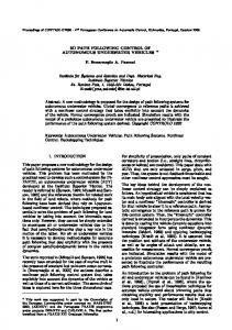
current has a component acting in the direction normal to the path, an underactuated vessel such as (6) cannot stay identically on the path y = 0 with zero heading. This is a major drawback that results in deviation problems when using LOS control in the presence of disturbances. Instead the vessel must be allowed to side-slip such that a component of the forward velocity of the vessel can counteract the effect of the ocean current. In particular, this implies that the vessel must have a non-zero heading in order to move along the path, see Fig. 1. This is the motivation for this paper: to develop an improved LOS design that handles ocean currents by automatically creating the reference heading angle that produces the necessary side-slip. P

B. Integrative LOS Guidance As discussed in Section III, traditional LOS guidance is simple and intuitive and has several nice properties. However, traditional LOS guidance is not designed to handle ocean currents or any other environmental disturbances such as wind or waves. To this end, we propose a modified LOS guidance law with integral action:

 y + σyint m −1 ψLOS  − tan , Δ > 0. (11a) Δ Δy . (11b) y˙ int = (y + σyint )2 + Δ2

ψ U vc

Fig. 1.

looses control and drifts away with the current. Assumption A.4 is a natural assumption for marine surface vessels, since Y > 0 would imply that the vessel is open-loop unstable in sway, which is not the case in practice. Remark: Note that a marine surface vessel can be openloop unstable in sway-yaw, e.g. course unstable vessels. However, a vessel cannot be open-loop unstable in the sense that Y (ur ) > 0, since this would imply that the system is not passive. A small perturbation in sway would then result in an accelerating sway velocity, which is not a realistic response for a marine vessel.

Path following in the presence of currents.

IV. C ONTROL S YSTEM In this section, we present the control system that solves the control problem stated in Section II-B. The proposed control strategy consists of three components: a modified LOS guidance law with integral action, an adaptive yaw tracking controller for tracking the desired heading provided by the guidance law and an adaptive surge tracking controller for tracking a desired surge speed profile. In this section, we present the control laws and analyze the closed loop tracking error dynamics. In Section V, we provide the conditions under which the proposed control strategy meets the control goals (7)-(9). Before we present the controllers, we state the assumptions on which the controller design will be based.

Here, σ > 0 is a design parameter, an integral gain, and Δ has the same interpretation as in the case of traditional LOS guidance, see Section III. The idea behind (11) is that m the integral of the cross-track error y will allow ψLOS to be non-zero when y = 0, i.e. when the vessel is on the desired path. In particular, in the presence of disturbances driving the system away from its path, the integral of the cross-track error m . When the vessel y will build up to create a non-zero ψLOS is on the desired path, the integral term will generate the necessary side-slip angle to follow the path. These statements will be made clear in Section V. P

A. Assumptions The controller design presented and analyzed in the next sections will be based on the following assumptions: A.1: The ocean current is irrotational and constant in the inertial frame, i.e. v c = [Vx , Vy , 0]T , where v˙ c = 0. A.2: The ocean current intensity has a known upper bound Vmax > 0, i.e. ||v c ||2 = Vx2 + Vy2 ≤ Vmax < ∞.

ψd ψ

Δ x

σyint Fig. 2.

y

Illustration of modified LOS guidance.

The desired constant speed Ud is strictly greater than the ocean current intensity, i.e. Ud > Vmax . Remark: Note that Eq. (11b) has the property that y˙ int → A.4: The function Y (ur ) satisfies 0 as y → ∞. This means that the rate of integration will decrease with large cross-track errors. In particular, the Y (ur ) ≤ −Ymin < 0, ∀ur ∈ [−Vmax , Ud +Vmax ]. integral term will be less dominant when the cross-track error Assumption A.1 is a simplification of the real world situation. is large, i.e. when the vessel is far from the desired path. This Assumption A.2 will be used when deriving stability criteria property will reduce the risk of integrator wind-up and reduce and Assumption A.3 is necessary to avoid that the vessel performance limitations related to integrator wind-up. A.3:

4986

47th IEEE CDC, Cancun, Mexico, Dec. 9-11, 2008

ThB16.5

To make u → ud , we propose the following adaptive surge controller: To guide the vessel towards the desired path, we control  the yaw angle ψ of the vessel to the desired yaw angle ψd  1 d11 (m22 v + m23 r)r + ud τu = − m m ψLOS , where ψLOS is given by the modified LOS guidance m11 m11

law (11). This is done using the adaptive yaw controller −φTu (ψ, r)θˆu + u˙ d − ku (u − ud ) , (16a) τr = −Fr (u, v, r) − φTr (u, v, r, ψ)θˆr + ψ¨d ˙ θˆu = γu φu (ψ, r)(u − ud ). (16b) − (kψ + λkr )(ψ − ψd ) − (kr + λ)(r − ψ˙ d ), (12a)

θˆ˙ r = γr φr (u, v, r, ψ) (r − ψ˙ d ) + λ(ψ − ψd ) . (12b) Here, ku > 0 is a constant controller gain and γu > 0 is a constant adaptation gain. As follows from Eq. (6a), Here, λ, kψ , kr > 0 are constant controller gains and γr > the controller (16) is an adaptive feedback linearizing P0 is a constant adaptation gain. As follows from Eq. (6c), controller. Similar to the controller (12), the controller (16) the controller (12) is an adaptive feedback linearizing PD- does not depend on the relative velocities, which are not controller. Note that the controller (12) does not depend on available for feedback. the relative velocities, which are not available for feedback. We define the errors u ˜  u − ud and θ˜u  θˆu − θu . We define the errors ψ˜  ψ − ψd , s  ψ˜˙ + λψ˜ and θ˜r  Using (6a), (16a) and (16b), we then derive the closed loop ˜ s and θ˜r , and using dynamics of the errors u ˜ and θ˜u : θˆr − θr . Taking the time-derivative of ψ,

 (1c), (6c), (12a) and (12b), then gives d11    ˙    T  u ˜=− + ku u (17a) ˜ − φTu (ψ, r)θ˜u , ˙ ˜ ˜ m 0 −λ 1 ψ 11 ψ = ˜ θ . (13a) − r ˙ −kψ −kr s φTr s˙ θ˜u = γu φu (ψ, r)˜ u. (17b) ˙ ˜ θr = γr φr (u, v, r, ψ)s. (13b) To analyze the stability properties of the interconnected system (17), we consider the time-derivative of the posiTo analyze the stability properties of the interconnected tive definite and radially unbounded LFC Vu  1/2˜ u2 + system (13), we consider the time-derivative of the positive T definite and radially unbounded Lyapunov function candidate 1/(2γu )θ˜u θ˜u along the solutions of system (17). This gives T

 (LFC) Vψ  1/2kψ ψ˜2 + 1/2s2 + 1/(2γr )θ˜r θ˜r along the d11 ˙ Vu = − + ku u (18) ˜2 ≤ 0. solutions of system (13). This gives m11 V˙ ψ = −λkψ ψ˜2 − kr s2 ≤ 0. (14) From Eq. (18) it follows that V˙ u is negative semi-definite From Eq. (14) is follows that V˙ ψ is negative semi-definite on Du = R × R2 and it hence follows, from standard on Dψ = R2 × R5 . It hence follows, from standard Lya- Lyapunov arguments, that the origin (˜ u, θ˜u ) = (0, 0) is a ˜ ˜ UGS equilibrium point of the interconnected system (17). punov arguments, that the origin (ψ, s, θr ) = (0, 0, 0) is a uniformly globally stable (UGS) equilibrium of the intercon- Moreover, it is again straightforward using, for example, ˜(t) → 0 asymptotically nected system (13). Note that system (13) is non-autonomous. Barbalat’s Lemma, to conclude that u ˜(t) ∈ L2 . Again, the equilibrium is not Hence, LaSalle’s invariance principle is not applicable in this as t → ∞ and that u case. However, it is straightforward to apply, for example UGAS, since the regressor φu (ψ, r) is not PE. ˜ s) → (0, 0) asymptotBarbalat’s Lemma, to conclude that (ψ, ˜ V. M AIN R ESULT ically as t → ∞ and that ψ(t), s(t) ∈ L2 . Note that we cannot ˜ s, θ˜r ) = (0, 0, 0) is hope to show that the equilibrium (ψ, In this section, we present the main technical result of the UGAS, since the regressor φr (u, v, r, ψ) is not persistently paper. In particular, we state the conditions under which the exciting (PE). A persistently exciting regressor is a necessary control goals (7)-(9) are achieved using the control strategy condition for UGAS of adaptive systems such as (13) (see presented in the previous section. e.g. [7]). Finally, note that asymptotic convergence of ψ˜ and Before we state the main result, we introduce the following s to zero also implies asymptotic convergence of r to ψ˙ d , notation: since (r − ψ˙ d ) = s − λψ˜ by definition. ¯ max  max (|X(ur , uc ) − uc |) , X (19) D. Surge Control Ω C. Yaw Control

The control goal (9) is to control the total speed U of where X(ur , uc ) is given by (52b) in Appendix A and the vessel to the desired constant value Ud . To this end, we Ω = {−Vmax < ur < (Ud + Vmax ), |uc | < Vmax }. (20) choose the desired surge speed as ud  Ud cos ψd ,

(15) With this notation, we now formulate the main technical result of the paper. where ψd ∈ (−π/2, π/2) is the desired heading given by Eq. (11a). The motivation behind (15) will become clear in Theorem 1. Consider an underactuated vessel described by the dynamic system (6). If Assumptions A.1-A.4 hold, and if Section V.

4987

47th IEEE CDC, Cancun, Mexico, Dec. 9-11, 2008

ThB16.5

the look-ahead distance Δ of the guidance law (11) satisfies s, then gives the condition Δy  (26) y˙ int = ¯ max

σ2 X Ud + Vmax + σ (y + σyint )2 + Δ2 + Δ> 1+ , (21) Ymin Ud − Vmax − σ 2 y + σyint Δ + vr  y˙ = −ud  2 + Δ2 2 2 (y + σy ) (y + σy int int ) + Δ where the integral gain σ satisfies the condition Δ + vc  Y min 1 2 2 ΔX (y + σy int ) + Δ ¯ max (Ud +Vmax )2 (U − V ) < σ < (U − V ), d max d max T min Y 1 + hy (ud , vr , vc , ψd , ξ)ξ (27) 1 + ΔX ¯ max (Ud +Vmax )2 T (22) ¯ r , uc )ψ˙ d + Y (ur )vr + hv (ur , uc , ξ)ξ. v˙ r = X(u (28) r then the controllers (12) and (16), where ψd is given by (11a) and ud is given by (15), guarantees that the control goals (7)- Here, ξ  [˜ ˜ s]T is a vector of converging error signals u, ψ, T (9) are achieved. In particular, control goal (8) is achieved and h (ud , vr , vc , ψd , ξ)ξ and hT (ur , uc , ξ)ξ contain all y vr with terms vanishing at ξ = 0. The expressions of hy and hvr

 Vy ∗ ψss = − tan−1 . (23) are given in Appendix A.  ψss Ud + Vx Notice that the current component vc , expressed in bodyframe coordinates, can be expressed using the constant inerProof. The proof of this theorem is given in Section VI. tial ocean current components Vx and Vy according to Remark: Note that it is always possible to satisfy condition vc = −Vx sin ψ + Vy cos ψ. (29) (22), since the left-hand side of the inequality is always strictly less than the right-hand side. Substituting this expression for vc in (27) and using Equations ˜ then gives Remark: It is interesting to note that in the case of no (11a), (15) and the expression ψ = ψd + ψ, currents and no integral action in the guidance law, i.e. setting Δy σ = 0 in (11a), then the condition on the look-ahead distance y˙ int = (30a) Δ, given in Eq. (21), reduces to the condition found in [8], (y + σyint )2 + Δ2 where the traditional LOS guidance law (10) was used to y + σyint y˙ = −Δ(Ud + Vx ) achieve path following of a straight-line path for the case of (y + σyint )2 + Δ2 no currents. Δ2 + Vy Remark: The proposed controllers (12) and (16) rely on (y + σyint )2 + Δ2 feedback linearization. If the model parameters have a high Δ + vr  degree of uncertainty, other control approaches may be bet(y + σyint )2 + Δ2 ter suited. Handling uncertain parameters in the controllers ˆ Ty (Ud , vr , vc , ψd , ξ)ξ remain a topic for future work. +h (30b) T ¯ r , uc )ψ˙ d + Y (ur )vr + h (ur , uc , ξ)ξ. (30c) v˙ r = X(u vr VI. P ROOF OF T HEOREM 1 ˆ y1 , h ˆ y2 , h ˆ y3 ]T are given in ˆ y  [h The expression for h We start the proof of Theorem 1 by considering the dynamAppendix A. ics of the cross-track error y and the relative sway velocity It is straightforward to verify that the equilibrium point of vr . From the analysis presented in Sections IV-C and IV-D, system (30), on the manifold ξ = 0, is given by ˙ we know that u → ud , ψ → ψd , r → ψd asymptotically ˜ as t → ∞ and that the error variables ψ(t), s(t), u˜(t) ∈ L2 . Δ Vy eq yint =  yint , y = 0, vr = 0. (31) Using Equations (2), (6b) and the expressions u = ud + u˜, σ Ud + Vx ˜ ˙ ˜ v = vr + vc , ψ = ψd + ψ and r = ψd + (s − λψ), the crosstrack error dynamics (1b) and the dynamics of the relative Hence, Vy can be written in terms of the equilibrium point eq sway velocity vr can then be written as yint according to ˜ y˙ = −(ud + u ˜) sin(ψd + ψ) ˜ + (vr + vc ) cos(ψd + ψ)

(24)

Vy =

σ eq (Ud + Vx )yint . Δ

(32)

v˙ r = v˙ − v˙ c = X(ur , uc )r + Y (ur )vr − (−uc r) To proceed, we define a new set of coordinates ˜ + Y (ur )vr . ¯ r , uc )(ψ˙ d + (s − λψ)) = X(u (25) eq (33a) z1  yint − yint ¯ r , uc )  X(ur , uc ) − uc . Substituting (11a) for ψd Here, X(u (33b) z2  y + σz1 . in the above equations, extending the state space with (11b) and factorizing the result with respect to the errors u ˜, ψ˜ and Taking the time-derivative of (33a) and (33b) and using (30)

4988

47th IEEE CDC, Cancun, Mexico, Dec. 9-11, 2008 and (32), we obtain the transformed dynamics z2 − σz1 z˙1 = Δ eq 2 (z2 + σyint ) + Δ2 z2 z˙2 = −Δ(Ud + Vx ) eq 2 (z2 + σyint ) + Δ2 Δ + vr  eq 2 (z2 + σyint ) + Δ2 z2 − σz1 + σΔ eq 2 (z2 + σyint ) + Δ2 ˆ y (Ud , vr , vc , ψd , ξ)ξ +h ¯ r , uc )ψ˙ d + Y (ur )vr + hTv (ur , uc , ξ)ξ, v˙ r = X(u r T

ThB16.5 after using the notation (19) and Assumption A.4. To simplify the above expressions, we eq 2 (34a) define z¯ 2 and z  |z |/ (z + σy ¯2  1 1 2 int ) + Δ  eq 2 2 |z2 |/ (z2 + σyint ) + Δ . With this notation, V˙ can be bounded according to

 σ2 ¯ V˙ ≤ − Δσ 3 − κ 2 X z1 |2 max |¯ 2Δ − Δ (Ud − Vmax − σ) |¯ z2 |2

 ¯ max X + Δ 1 + κ 2 (Ud + Vmax + σ) |¯ z2 ||vr | (34b) Δ

 1 ¯ σ2 ¯ (34c) − κ Ymin − X (42) Xmax |vr |2 . max − Δ 2Δ

Now, substituting the expression



eq  Furthermore, choosing κ equal to (we will show that κ > 0 z2 + σyint d −1 ˙ ψd = − tan in the following) dt Δ 2α − 1 Δ κ  X¯ , (43) =− z˙2 , (35) eq 2 2 max (z2 + σyint ) + Δ Δ2 (Ud + Vmax + σ) in (34c), where z˙2 is given by (34b), we finally obtain where α is given by ⎡ ⎤ ⎤ ⎡ z˙1 z1 ¯ max ¯ max − σ2 X ΔYmin − X ⎣ z˙2 ⎦ = A(z2 , ur , uc ) ⎣ z2 ⎦ + H(t, z2 , vr , ξ)ξ, (36) 2 , (44) α  (Ud − Vmax − σ) ¯ Xmax (Ud + Vmax + σ) v˙ r vr where A(z2 , ur , uc ) is given by Eq. (38) and gives the following bound for V˙ : ⎤ ⎡

 0 σ2 ¯ 3 ˙ T V ≤ − Δσ X − κ |¯ z1 |2 ⎥ ⎢ ˆ 2 max h 2Δ H(t, z2 , vr , ξ)  ⎣ . (37) ⎦ y r ,uc ) ˆ Ty − Δ (Ud − Vmax − σ) |¯ z2 |2 + 2Δα|¯ z2 ||vr | h hTvr − (z2ΔX(u eq 2 2 +σyint ) +Δ α(2α − 1) The next lemma characterizes the stability properties of the |vr |2 . (45) −Δ Ud − Vmax − σ nominal system ⎤ ⎤ ⎡ ⎡ z1 z˙1 Defining β  Ud − Vmax − σ (we will show that β > 0 in ⎣ z˙2 ⎦ = A(z2 , ur , uc ) ⎣ z2 ⎦ . (39) the following), we can finally bound V˙ according to

 v˙ r vr σ2 ¯ 3 ˙ V = − Δσ − κ 2 Xmax |¯ z1 |2 Lemma 1. Under the conditions of Theorem 1, the nominal 2Δ   system (39) is UGAS and ULES.    Δβ −Δα |¯ z2 | | |v | |¯ z − (46) 2 r Proof. To analyze the stability properties of the nominal |vr | −Δα Δ α(2α−1) β system (39), we consider the time-derivative of the positive  −W (|¯ z1 |, |¯ z2 |, |vr |). (47) definite and radially unbounded LFC 1 2 1 1 z1 |, |¯ z2 |, |vr |) is positive definite, or V  σ |z1 |2 + |z2 |2 + κ|vr |2 , κ > 0, (40) To guarantee that W (|¯ 2 2 2 equivalently that V˙ is negative definite, we must guarantee along the solutions of system (39). This gives ¯ max . By simple that α > 1, β > 0 and σ > κ/(2Δ)X 2 manipulation, one can easily check that condition (21) implies Δ|z | 1 V˙ ≤ −σ 3 eq 2 2 that α > 1. Note that this also implies that κ > 0, as (z2 + σyint ) + Δ

 required for V to be positive definite. Furthermore, β > 0 (Ud − Vmax ) − σ 2 −Δ | |z 2 eq 2 is guaranteed by Assumption A.3 and the upper bound on σ (z2 + σyint ) + Δ2 ¯ max , notice that κ from (22). To check that σ > κ/(2Δ)X Δ can be upper bounded according to + |z2 ||vr | eq 2 (z2 + σyint ) + Δ2 Ud − Vmax − σ 2α ¯ max κ < X¯ < 2Δ3 Ymin ¯ 2 . σ 2 Δ2 X max +κ Xmax (Ud + Vmax )2 2 |vr ||z1 | 2 (Ud + Vmax ) eq 2 Δ 2 ((z2 + σyint ) + Δ ) Using this upper bound on κ and the lower bound on σ ¯ max Δ2 X (Ud + Vmax ) + σ ¯ max . +κ |z ||v | 2 r from (22) one can easily check that σ > κ/(2Δ)X eq 2 eq 2 (z2 + σyint ) + Δ2 (z2 + σyint ) + Δ2 ˙ is negative definite and it follows, from stan

 Hence, V ¯ max Δ2 X |vr |2 , (41) dard Lyapunov arguments, that the nominal system (39) − κ Ymin − eq 2 ((z2 + σyint ) + Δ2 )3/2 is UGAS. At the same time, note that the function W

4989

47th IEEE CDC, Cancun, Mexico, Dec. 9-11, 2008 ⎡

− (z2 +σyσΔ eq 2 ) +Δ2

int σ2 Δ eq 2 (z2 +σyint ) +Δ2 2 2 ¯ σ Δ X(ur ,uc ) eq 2 ((z2 +σyint ) +Δ2 )2

⎢ − A(z)2  ⎢ ⎣

ThB16.5

Δ eq 2 (z2 +σyint ) +Δ2 (Ud +Vx )−σ −Δ (z2 +σyeq )2 +Δ2 int ¯ r ,uc ) Δ2 X(u (Ud +Vx )−σ eq 2 eq 2 (z2 +σyint ) +Δ2 (z2 +σyint ) +Δ2

¯ 1 |¯ ¯ 2 |¯ satisfies W (|¯ z1 |, |¯ z2 |, |vr |) ≤ λ z1 |2 + λ z2 |2 + λ3 |vr |2 , ¯ ¯ for some constants λ1 , λ2 , λ3 > 0. Moreover, in any ball Br {|z2 | ≤ r}, r > 0, the function W (|¯ z1 |, |¯ z2 |, |vr |) can be estimated as W ≤ λ1 |z1 |2 + λ2 |z2 |2 + λ3 |vr |2 , where ¯ i /((r + σy eq )2 + Δ2 ), i = 1, 2. This, together with λi = λ int the fact that V is a quadratic function of z1 , z2 and vr , implies that the nominal system (39) is uniformly exponentially stable in any ball Br (see e.g. [9]). This concludes the proof of Lemma 1.

⎤

0

⎥ Δ √ ⎥ eq 2 (z2 +σyint ) +Δ2 ⎦   2 ¯ Δ X(ur ,uc ) Y (ur ) − ((z2 +σy eq 2 ) +Δ2 )3/2

(38)

int

∗ in the above equation Inserting the expression (23) for ψss and rearranging then gives  Ud2 (Vy2 + (Ud + Vx )2 ) lim U (t) = = Ud . (51) t→∞ Vy2 + (Ud + Vx )2

Hence, control goal (9) is also achieved. This concludes the proof of Theorem 1. VII. C ONCLUSIONS

In this paper, we have considered the development of a control strategy for path following of underactuated marine surface vessels in the presence of constant, irrotational ocean currents. In particular, we have proposed a control strategy based on a modified LOS guidance law with integral action and a pair of adaptive tracking controllers. This approach preserved the simplicity and interpretation of traditional LOS guidance, while ensuring sufficient countermeasures against Lemma 2. Under the conditions of Theorem 1, the solutions environmental disturbances. The closed-loop dynamics was of system (36) are globally bounded. analyzed in detail and explicit conditions for global asymptotic path following were derived. Proof. The proof of this lemma is given in Appendix B.

We have thus proved that the nominal system (39) is UGAS and ULES under the conditions of Theorem 1. It now remains to analyze the interconnected system of (36) and the dynamics of ξ, i.e. systems (13a), (17a) and to show that the control goals (7)-(9) are achieved. The next lemma shows that the solutions of system (36) are globally bounded under the perturbation from the L2 -signal ξ(t).

According to Lemma 2, the solutions z1 (t), z2 (t) and vr (t) of system (36) are globally bounded. Then, since ξ(t) → 0 asymptotically as t → ∞, it follows that z1 (t) → 0, z2 (t) → 0 and vr (t) → 0 asymptotically as t → ∞ (see [10]). Since both z1 and z2 converges asymptotically to zero, it follows from (33b) that y converges asymptotically to zero. Hence, it follows that control goal (7) is achieved. Moreover, using (31) in the expression

eq  z2 + σyint ˜ ψ = ψd + ψ˜ = − tan−1 + ψ, (48) Δ and using the fact that z2 → 0, ψ˜ → 0 asymptotically as t → ∞, it follows that

 Vy −1 ∗ . (49) lim ψ(t) = − tan = ψss t→∞ Ud + Vx

A PPENDIX A 

mA − mA d11 22 cos ψ − 11 r sin ψ, m11 m11 T d11 mA − mA 22 sin ψ + 11 r cos ψ , m11 m11 1 m33 (−d23 − m11 ur − mRB X(ur , uc )  11 uc ) Γ  RB +m23 d33 + m23 (m23 ur + m23 uc + mA 22 uc ) 1 Y (ur )  [−m33 d22 + m23 d32 Γ  A +m23 (mA 22 − m11 )ur , m22 [−(m22 v − m23 r)u + m11 uv Fr (u, v, r)  Γ m23 −d32 v − d33 r] − [−m11 ur − d22 v − d23 r] . Γ φu (ψ, r) =

(52a)

(52b)

(52c)

(52d)

∗ Hence, control goal (8) is achieved with ψss given by ψss , Here, Γ  m22 m33 − m223 > 0. Furthermore, the function φr (u, v, r, ψ)  [φr1 , . . . , φr5 ]T is defined by: cf. Eq. (23).      Next we show that control goal (9) is achieved. Utilizing cos ψ − sin ψ a1 φr1 the expression (29) for vc and using that u˜ → 0, vr → 0 and = (53) sin ψ cos ψ φr2 a2 ∗ that ψ → ψss , we have that m22 A (m11 − mA φr3 = − (54) 22 ) sin ψ cos ψ,  Γ 2 2 ˜) + (vr + vc ) lim U (t) = lim (ud + u m22 A t→∞ t→∞ φr4 = (55) (m11 − mA 22 ) sin ψ cos ψ, Γ ∗ 2 ∗ ∗ 2 = (Ud cos ψss ) + (−Vx sin ψss + Vy cos ψss ) . m22 A 2 (m11 − mA φr5 = (56) 22 )(1 − 2 sin ψ), (50) Γ

4990

47th IEEE CDC, Cancun, Mexico, Dec. 9-11, 2008

ThB16.5

Here,

 m23 A m22  A A A m11 r, a1 = − (m11 − mA 22 )v + (m23 − m22 )r − Γ Γ  m22  m 23 A d32 − (mA d22 . a2 = 11 − m22 )u − Γ Γ Remark: In deriving the expression (52c) we have used RB that mRB 11 − m22 = 0, which follows from the fact that RB RB m11 = m22 = m, where m is the mass of the vessel (see [6]). The functions hy  [hy1 , hy2 , hy3 ]T and hvr  [hvr 1 , hvr 2 , hvr 3 ]T are given by hy1 = − sin ψd , hy3 = 0, (57a) ˜ cos ψ − 1 hy 2 = (−(˜ u + ud ) sin ψd + (vr + vc ) cos ψd ) ψ˜ sin ψ˜ − ((˜ u + ud ) cos ψd + (vr + vc ) sin ψd ) , (57b) ψ˜ ¯ r , uc ), hvr 3 = X(u ¯ r , uc ). (57c) hvr1 = 0, hvr 2 = −λX(u ˆ y1 , h ˆ y2 , h ˆ y3 ]T is given by ˆ y  [h The functions h ˆ y1 = hy1 , h ˆ y2 h

ˆ y3 = hy3 , h (58a) sin ψ˜ (−Vx cos ψd − Vy sin ψd ) = hy2 + ψ˜ cos ψ˜ − 1 + (−Vx cos sind +Vy cos ψd ) . (58b) ψ˜

A PPENDIX B: P ROOF OF L EMMA 2 The perturbation ξ(t) is a vanishing perturbation to the system (36). In particular, ξ(t) → 0 asymptotically as t → ∞ and ξ(t) ∈ L2 , cf. Sections IV-C and IV-D. Hence, for any

> 0, there exists t∗ ≥ t0 + T , where T is not necessarily independent of t0 , such that ||ξ(t)|| ≤ , ∀t ≥ t∗ . Moreover, the time-derivative of the LFC (40) along the solutions of (36) can then be upper bounded by c2 c2 V ·||H||·||ξ||2 , t ∈ [t0 , t∗ ], (59) V˙ ≤ V ·||H||·||ξ|| ≤ c1 c1 where c1 ≤ 1/2 min{σ 2 , 1, κ} and c2 ≥ 1/2 max{σ 2 , 1, κ}. Using Equations (57), (58) and (37), it is straightforward to verify that the interconnection term H is globally bounded, i.e. that ||H|| ≤ bH , for some bH > 0. Using this, and integrating both sides of (59) from t0 to t∗ gives

  t∗  ∞ V (t∗ ) c1 ln ||ξ(s)||2 ds ≤ ||ξ(s)||2 ds. ≤ c2 b H V (t0 ) t0 t0 (60) Now, since ξ(t) ∈ L2 , the right hand side of (60) is bounded and it follows that V (t) is bounded on the interval [t0 , t∗ ]. In particular, there exits a constant c ≥ 0 such that V (t∗ ) = V (x(t∗ )) ≤ c, where x  [z1 , z2 , vr ]T . Using Eq. (47), the time-derivative of V can be see to satisfy z2 |, |vr |) + 2c2 ||x||bH , t ≥ t∗ , V˙ ≤ −W (|¯ z1 |, |¯ W (x) + 2c2 ||x||bH , t ≥ t∗ . ≤− ||x||2 + Δ2

Note that W (x) ≥ k1 ||x||2 for some k1 > 0, cf. Eq. (47). Thus, 1 W (x) 1 k1 ||x||2 V˙ ≤ − − + 2c2 ||x||bH (63) 2 ||x||2 + Δ2 2 ||x||2 + Δ2 1 W (x) k1 ≤− , ∀ ≤ . (64) 2 ||x||2 + Δ2 4c2 bH Hence, V˙ is negative on V (x) = c, and the set {V (x) = c} is positively invariant. Thus, for all x(t∗ ) ∈ {c2 ||x||2 ≤ c}, x(t) is bounded for all t ≥ t∗ . Moreover, since c > 0 is arbitrary, x(t) is globally bounded. This concludes the proof. R EFERENCES [1] A. Healey and D. Lienard, “Multivariable sliding-mode control for autonomous diving and steering of unmanned underwater vehicles,” IEEE Journal of Oceanic Engineering, vol. 18, no. 3, pp. 327–339, July 1993. [2] K. Y. Pettersen and E. Lefeber, “Way-point tracking control of ships,” in Proc. of 40th IEEE Conference on Decision and Control, Dec 2001, pp. 940–945. [3] T. I. Fossen, M. Breivik, and R. Skjetne, “Line-of-sight path following of underactuated marine craft,” in Proc. 6th IFAC Manoeuvring and Control of Marine Craft, Girona, Spain, Sep 2003, pp. 244–249. [4] M. Breivik and T. I. Fossen, “Path following for marine surface vessels,” in Proc. MTS/IEEE OCEANS ’04, 2004, pp. 2282–2289. [5] E. Fredriksen and K. Y. Pettersen, “Global κexponential way-point maneuvering of ships: Theory and experiments,” Automatica, vol. 42, no. 4, pp. 677– 687, 2006. [6] T. I. Fossen, Marine Control Systems. Trondheim, Norway: Marine Cybernetics, 2002. [7] A. Loria, R. Kelly, and A. R. Teel, “Uniform parametric convergence in the adaptive control of manipulators: a case restudied,” in Proc. ICRA ’03. IEEE International Conference on Robotics and Automation. IEEE, Sep 2003, pp. 1062–1067. [8] A. Pavlov, E. Børhaug, E. Panteley, and K. Y. Pettersen, “Straight line path following for formations of underactuated surface vessels,” in Proc. IFAC NOLCOS, Pretoria, South Africa, 2007, pp. 654–659. [9] H. Khalil, Nonlinear Systems, 3rd ed. Upper Saddle River, NJ, USA: Pearson Education International inc., 2000. [10] E. Sontag, “A remark on the converging-input converging-state property,” IEEE Transactions on Automatic Control, vol. 48, no. 2, pp. 313–314, Feb 2003.

(61) (62)

4991