detection and visual tracking to achieve better performance. Motion detection is ..... and weather conditions (shine, rain, and snow) of a large parking lot. In order ...
Integrated Motion Detection and Tracking for Visual Surveillance Mohamed F. Abdelkader Rama Chellappa Center for Automation Research (CfAR) University of Maryland, College Park, MD 20742
Qinfen Zheng
Alex L. Chan U. S. Army Research Laboratory (ARL) Adelphi, MD
Abstract Visual surveillance systems have gained a lot of interest in the last few years. In this paper, we present a visual surveillance system that is based on the integration of motion detection and visual tracking to achieve better performance. Motion detection is achieved using an algorithm that combines temporal variance with background modeling methods. The tracking algorithm combines motion and appearance information into an appearance model and uses a particle filter framework for tracking the object in subsequent frames. The systems was tested on a large ground-truthed data set containing hundreds of color and FLIR image sequences. A performance evaluation for the system was performed and the average evaluation results are reported in this paper.
1 Introduction In the last few years, visual surveillance has become one of the most active research areas in computer vision, especially due to the growing importance of visual surveillance for security purposes. Visual surveillance is a general framework that groups a number of different computer vision tasks aiming to detect, track, and classify objects of interest from image sequences, and on the next level to understand and describe these objects behavior. The ultimate goal in designing smart visual surveillance systems is to replace the existing passive surveillance and to remove, or at least, minimize the need for a human observer to monitor and analyze the visual data. For these reasons, there has been a number of wellknown visual surveillance systems– see [1] for an excellent survey. The real-time visual surveillance system W 4 [2] detects and tracks multiple people and monitors their activi-
ties in an outdoor scene using a single monocular gray-scale or IR camera. It uses a combination of shape analysis and tracking to locate people and their parts, and to create models of their appearance such that they can be tracked through interactions as occlusions. The Pfinder system developed by Wren et al [3] builds a 3D description model of a single unoccluded person in a large room using a fixed camera. CMU developed a surveillance system [4] that detects and tracks moving objects over a large area using a network of video sensors; detected objects are classified into categories using shape and color analysis. MIT’s system [5] first observes moving objects in a site using a distributed set of sensors, and then uses these observations to learn and classify patterns of activity in the scene that are later used to detect unusual activities. In this paper, we present an integrated visual surveillance system to monitor an outdoor scene through a stationary forward-looking infra-red (FLIR) or a color camera. Our system begins with the motion detection module, which is responsible for detection and segmentation of moving objects, as well as initializing the tracker. The tracking module estimates the new location of the object at each new frame and maintains the object identity. The performance evaluation module is used to evaluate the system performance using the available ground truth data. The main features of our system are as follows: • Motion detection algorithm that integrates both temporal variance and background modeling to allow for a robust detection of moving objects. • An adaptive visual tracking algorithm using both appearance and motion observations in a statistical framework. Particle filters are used in the state estimation to accommodate for appearance changes. The tracking algorithm adaptively updates motion velocity, appearance, noise, and number of particles at each new
Proceedings of the Fourth IEEE International Conference on Computer Vision Systems (ICVS 2006) 0-7695-2506-7/06 $20.00 © 2006 IEEE
frame. • The integration of the motion detection and tracking stages by using the motion detection module for initialization of the appearance model for the visual tracker, and for obtaining the motion observation. • Performance evaluation module responsible for measuring and evaluating the performance of the system with respect to a ground- truthed detection data set. The remainder of the paper is organized as follows. In Section 2, we describe our motion detection algorithm. Section 3 focuses on the process of object tracking using both appearance and motion information. Section 4 presents the performance evaluation of our system. Conclusions are provided in Section 5.
2 Moving-Object Detection The detection of moving objects is the first stage of a typical surveillance system. Motion detection aims at segmenting the regions pertaining to moving objects from the rest of the image. Subsequent processes such as tracking and behavior analysis are greatly dependent on the performance of this stage. Many algorithms have been suggested to solve the problem of motion detection, most of which can be categorized into three main approaches: temporal thresholding as in [6], where the moving pixels are identified by thresholding the temporal difference between the frames; background subtraction where detection occurs by comparing the incoming frame with a background model of the scene that is built by modeling the pixel intensity either by a single Gaussian distribution [3], a mixture of Gaussians [5], or using the maximum, minimum and maximum intensity difference as in [2]; and optical flow approaches [7] that use characteristics of flow vectors of moving objects over time to detect moving regions in image sequences. We present a method based on combining both the temporal variance of the pixel intensities as temporal thresholding approach with background modeling to achieve a robust and accurate motion detection and to reduce false alarms. Our approach is suitable for both color and FLIR sequences collected by stationary surveillance cameras, which are most commonly used in surveillance systems.
2.1
Temporal Variance Based Motion Detection
In our system, we use the temporal variance as a parameter to detect moving areas in a stationary scenes as in [8] and [9]. The mean and variance of the intensity value at each pixel is calculated over a window of several previous
frames and updated recursively for every new frame. This value of the variance is used directly afterward for the detection of moving area. The use of temporal variance for motion detection has some nice properties: 1. The variance of intensity at a certain pixel depends on both the amplitude of changes and the duration of this change so it is more robust to transient noises incurred by moving texture. 2. There is no need for background training period as this method can build the model with the existence of moving objects on the scene. The mean and variance for the intensity at each pixel (i, j) are recursively updated using a simple exponentially decaying adaptive filter as follows: m(i, j, t) = m2 (i, j, t) = σ 2 (i, j, t) =
αm(i, j, t − 1) + (1 − α)x(i, j, t) αm2 (i, j, t − 1) + (1 − α)x2 (i, j, t) m2 (i, j, t) − m2 (i, j, t)
(1)
where: x(i, j, t) is the intensity, m(i, j, t) is the first moment, m2 (i, j, t) is the second moment and σ 2 (i, j, t) is the variance at pixel (i, j) at time t, α is the decay rate, that can be rewritten with respect to the filter window size N as: α=
1 N −1 ;N = N 1−α
(2)
The main problem with using the variance is that it takes a while for the variance to decay back to its original value after the change has ended. This problem causes the moving object to leave a trail behind it, consisting of pixels that were in motion in the proceeding frames. The variance decay rate can be controlled by changing the window size N , however, reducing this size will make the model too adaptive to any changes in the scene. To overcome this problem we propose using a simple background model, which is adaptively updated, to remove this trail effect.
2.2
Background modeling
In order to remove the trail effect, a background model is built by recursively updating another set of mean and variance as follows: mbg (i, j, t) m2bg (i, j, t) 2 σbg (i, j, t)
= αbg mbg (i, j, t − 1) + (1 − αbg )x(i, j, t) = αbg m2bg (i, j, t − 1) + (1 − αbg )x2 (i, j, t) = m2bg (i, j, t) − m2bg (i, j, t)
(3)
where: mbg (i, j, t) is the background first moment, m2bg (i, j, t) is the background second moment, and σbg (i, j, t)2 is the background variance for the background
Proceedings of the Fourth IEEE International Conference on Computer Vision Systems (ICVS 2006) 0-7695-2506-7/06 $20.00 © 2006 IEEE
at pixel (i, j) at time t. αbg is the background model decay rate that can also be written with respect to the background filter window size Nbg in the same way shown in Equation(2). The difference between the two models is: • The window size used for the background model Nbg is much larger than that used for the variance update, so that the background model is slowly varying and covers a longer history of the frames.
(a)
• The update process for the background model is selective in the sense that only pixels that have not been identified as possible foreground pixels, using the variance, are incorporated at each new frame. So we may assure that this background model does not include any foreground object. The background model is used to obtain a confidence weight representing the confidence of this pixel being a part of the foreground. This confidence weight is obtained as a function of the distance between the pixel intensity and the background model � � |x(i, j, t) − mbg (i, j, t)| � C(i, j, t) = f (4) σbg (i, j, t) where C(i, j, t) is the confidence weight that the pixel (i, j) is part of the foreground and f is a nonlinear-mapping function– such as sigmoid– to map the distance to range of [0,1] and to emphasize the large distance points. The final binary detection map L(i, j, t) is obtained as follows: � 1 if C(i, j, t)σ(i, j, t) ≥ T hreshold L(i, j, t) = 0 if C(i, j, t)σ(i, j, t) < T hreshold (5) where the value of Threshold can be obtained either empirically or by multiplying the average background variance by a factor.
2.3
Motion Segmentation
The motion segmentation could be considered as the interface between motion detection and tracking stages of the surveillance system. It includes the segmentation of the moving areas from the binary detection map into disjoint objects, the removal of any small or isolated noise, and the initialization of the bounding boxes that are passed to the subsequent tracker. In order to perform these tasks, we use the connectedcomponent labeling algorithm presented in [10]. This algorithm performs several raster passes on the binary image L(t) and uses sequential local operations with a one-dimensional table, which produces a fast connectedcomponent result. After the labeling, a bounding box containing all the pixels with the same label is drawn. These
(b)
(c) Figure 1. The motion detection stages .(a) The square root of the variance image showing the trails left by the moving objects,(b) The foreground confidence map with the more bright the area the more likely it is a foreground object and (c) The final motion detection map after multiplying (a) and (b) and applying the threshold
bounding boxes are sent to the subsequent tracker in order to start the tracking process.
3 Object tracking Object tracking module is responsible for estimating the location of each object in each new frame. This module ensures that the object is being tracked even if the motion detection module fails to detect it, either due to occlusion or stopped object. As a problem of interest for a long time, visual tracking research can be categorized into four main categories [1]; region-based, active-contour-based, feature-based, and model-based tracking. Our tracker belongs to the fourth category, in which we build a model for the tracked object and search for the best match for this model in subsequent frames. Different models have been used, such as: stick figures [11], 2-D contour [12], and appearance models [17]. Different search strategies have been employed to search for the best match, either deterministic by minimizing a cost function as in [13], or probabilistic aiming to estimate the motion state for a state space model using an estimation tool like Kalman filter [14] and Condensation algorithm [15]. In our surveillance system we use a tracking algorithm based on the work presented in [16]. We design a new ob-
Proceedings of the Fourth IEEE International Conference on Computer Vision Systems (ICVS 2006) 0-7695-2506-7/06 $20.00 © 2006 IEEE
servation model that incorporates both appearance and motion information of the object. This algorithm appears to be very effective and robust even in challenging tracking conditions like static occlusion and cluttering background. The tracking problem can be formulated as an estimation process, where the goal is to estimate the unknown motion state θt from a noisy collection of observations, Y1:t = {Y1 , . . . Yt } arriving in a sequential fashion. For each observed frame Yt , different image patches Zt correspond to different motion states θt by the relation Zt = T{Yt ; θt }, where T is the motion transformation used (Affine in our case). The system transition is usually modeled using a state space model with two important components, the state transition and observation models, which are generally expressed as: state transition model :
θt
Observation model : Yt
= Ft (θt−1 , Ut ),
(6)
= Gt (θt , Vt ),
(7)
where Ut is the system noise, Ft (. . .) characterizes the kinematics, Vt is the observation noise, and Gt (. . .) models the observer. Due to the nonlinear and non-Gaussian nature of our system model; the particle filter [18] is used as a powerful technique to approximate the posterior distribution (j) (j) p(θt |Y1:t ) by a set of weighted particles {θt , wt }Jj=1 . Then the state estimate θˆt can be calculated as a maximum a posteriori (MAP) estimate [18]. (j) θˆt = θtmap = arg max p(θt |Y1:t ) ≈ arg max wt θt
θt
(8)
or any other estimators based on p(θt |Y1:t ).
3.1
Adaptive State Transition Model
The state in our Model θt represent the affine motion parameters used in the system. The state transition model used in our system is a simple adaptive Markov model of the form θt = θˆt−1 + νt + Ut (9) where Ut is the system noise term and νt is the adaptive velocity. We provide a brief overview of the model the readers are refered to [16] for more details. 3.1.1 Adaptive Velocity Aside from the noise term, the adaptive velocity term νt �= θt − θˆt−1 is predicted using a first-order linear approximation of the constant brightness constraint. A least square solution is found via using the difference between the incoming observation Yt and the previous set of observations (j) Zt−1 = {Zt−1 }Jj=1 .
3.1.2 Adaptive Noise and Number of Particles After calculating the velocity, the variance of the noise Ut and the number of particles in the particle filter are chosen to be proportional to the value of the residual error �t between the predicted patch Z˜t = T{Yt ; θˆt−1 + νt } and the appearance model. This value determines the quality of prediction. Therefore, if �t is small, implying a good prediction, we only need noise with small variance and small number of particles to absorb the residual motion and vice versa.
3.2
Appearance-Motion Adaptive Observation Model
We use an observation model that combines the motion information (background modeling) and appearance information (foreground modeling) to achieve more robustness especially in the cases where one of the two cues fails. We use the model presented in [19] to combine both cues and assume that the observation Yt is segmented by the motion state θt into two mutually exclusive and collectively exhaustive sets: β(θt ) and F (θt ), which are the regions identified by the state θt as background and foreground (target), respectively. With this assumption, the observation equation p(Yt |θt ) can be written as follows: p(Yt |θt ) = p(Yt (β(θt )), Yt (F (θt ))|θt ) = p(Yt (β(θt ))|θt )p(Yt (F (θt ))|θt ) (10) = p(Yt (β(θt ))|βt )p(Yt (F (θt ))|At ) Where At is the appearance model and βt is the background model. Under the assumption that the background is composed of independent pixels. p(Yt (β(θt )|θt )|βt ) =
p(Yt |βt ) p(Yt (F (θt ))|βt )
(11)
So the likelihood function p(Yt |θt ) can be written in the following way p(Yt |θt ) = p(Yt |βt )
p(Yt (F (θt ))|At ) p(Yt (F (θt ))|βt )
(12)
3.2.1 Appearance Modeling The appearance-based tracking relies on building an adaptive appearance model for the object and estimating the new location of this object in subsequent frames. Our appearance model [16] is an online adaptive appearance model At , which is a modified version from the online appearance model (OAM) developed in [17]. Mixture appearance model:we use a time varying OAM that consists of a mixture density of three components At = {Wt , St , Ft }. The W -component characterizes a
Proceedings of the Fourth IEEE International Conference on Computer Vision Systems (ICVS 2006) 0-7695-2506-7/06 $20.00 © 2006 IEEE
short time-course, such as in a two-frame tracker, so it is modeled as a Gaussian component that is conditioned on the estimated image patch from the last frame Zˆt−1 . The fixed template component F is modeled as a Gaussian with fixed mean and variance. Finally, the S-component depicts the stable structure, which is modeled by a slowly varying Gaussian component whose parameters are updated with every new frame to cope for the slow changes in the appearance over time. The observation likelihood is written as p(Yt (F (θt ))|At ) = p(Zt |θt ) =
d �
{
�
2 αi,t (j)N (Zt (j); mi,t (j), σi,t (j))},
(13)
j=1 i=w,s,f 2 ; i = w, s, f } and where: {mi,t ; i = w, s, f }, {σi,t {αi,t ; i = w, s, f } are the respective mixture means, variances, and mixing probabilities of the three densities, and N (x; m, σ 2 ) is a normal density of mean m and variance σ2 . Model Initialization and Update: The appearance model A1 is initialized by setting W1 = S1 = F1 = Z0 , where Z0 is the the initial area initialized by the detection module. The update of the appearance model At to At+1 is carried out using an Expectation-Maximization (EM) algorithm with the assumption that the past observations are exponentially ’forgotten’ with respect to their contribution to the current appearance model.
3.2.2 Motion Modeling The motion-based modeling in our observation model is formulated by defining a density function p(Yt (F (θt ))|βt ) and inserting it into the likelihood equation (12). For this purpose, we use the parameters of the background model introduced in the motion detection algorithm. Assuming that individual pixels are independent, p(Yt (F (θt ))|βt ) = p(Zt |βt ) =
d �
p(Zti |βt )
(14)
j=1
where p(Zti |βt ) is the probability distribution of the ith pixel of the patch under the background model. This distri2 2 bution is a Gaussian N (Zti ; mibg , σbg ), where σbg is a fixed variance indicating the level of confidence in the motion information and determining to what degree this information should contribute to the whole likelihood term.
4 Performance Evaluation The performance evaluation of surveillance systems has gained more interest in the last few years [20]. Most of the
Table 1. Average performance over the ARL data sequences Overall TRDR FAR Human TDR Vehicle TDR 82.13% 31.87% 94.09% 83.37%
research in this area is concerned with generating a meaningful error metric to be used in comparing the system results with the ground truth information. In this section we will provide an evaluation for the results obtained by testing our system on the force protection surveillance system (FPSS) dataset provided by U. S. Army Research Laboratory (ARL). The first set of this data consists of 85 FLIR and color sequences, all of which were manually ground-truthed with respect to the location and type of moving targets on each frame. These sequences represent a wide variety of views, complexity, day times and weather conditions (shine, rain, and snow) of a large parking lot. In order to evaluate the performance of our surveillance system we adopted some of the performance metrics used in [21] such as : Tracker Detection Rate (TRDR), False Alarm Rate (FAR), and Track Detection Rate (TDR) T otalT rueP ositives T otalN umberof GroundT ruthP oints T otalF alseP ositives F AR = T otalT rueP ositives + T otalF alseP ositives N umberof truepositivesf ortrackedobject T DR = T otalnumberof groundtruthpointsf orobject T RDR =
(15) Where a True Positive is defined as a ground truth point that is located within the bounding box of an object detected and tracked by the tracking algorithm. A False negative is a ground truth point that is not located with the bounding box of any object tracked by the tracking algorithm. A False positive is an object that is tracked by the system that does not have a matching ground truth point. (TRDR) and (FAR) characterize the overall tracking performance of the motion detection and object tracking algorithms for all the objects, while, TDR indicates the tracking completeness of a specific ground truth track. Because of the space limitation, we will just present the average evaluation result for all the sequences (Table.1).
5 Conclusion We have described a visual surveillance system that integrates motion detection and tracking tasks to achieve a better tracking performance. Temporal variance of pixel intensities is used for motion detection combined with
Proceedings of the Fourth IEEE International Conference on Computer Vision Systems (ICVS 2006) 0-7695-2506-7/06 $20.00 © 2006 IEEE
[5] W. E. L. Grimson, C. Stauffer, R. Romano, and L. Lee. Using adaptive tracking to classify and monitor activities in a site, in Proc. IEEE Conf. CVPR, Santa Barbara, CA, 1998, pp. 22-31.
(a)F rame42
(b)F rame98
Figure 2. Example for different object being tracked over time (Red boxes) along with the ground truth data where green, blue and yellow crosses represent human, vehicle, and other objects, respectively
background modeling to remove trail effect. We used a visual tracking algorithm that combines motion and appearance information into an observation model, uses an adaptive state transition model with adaptive velocity and noise, and uses particle filter as a tool for estimating the unknown state vector. The system was tested on a large data set of FLIR and color sequences collected by ARL FPSS program and the performance was evaluated with respect to manually ground-truthed data.
Acknowledgement This work was supported in part by the Advanced Sensors Consortium sponsored by the U.S. Army Research Laboratory under the Collaborative Technology Alliance Program, Cooperative Agreement DAAD19-01-2-0008
References [1] W. Hu,T. Tan,L.Wang, and S. Maybank. A survey on visual surveillance of object motion and behaviors, IEEE Trans. on systems, man, and cybernetics part C: Applications and Reviews, Vol.34, NO.3, AUGUST 2004. [2] I. Haritaoglu, D. Harwood, and L. S. Davis. W 4 : Realtime surveillance of people and their activities, IEEE Trans. PAMI, vol. 22, pp. 809-830, Aug. 2000. [3] C. R. Wren, A. Azarbayejani, T. Darrell, and A. P. Pentland. Pfinder: real-time tracking of the human body, IEEE Trans. PAMI., vol. 19, pp. 780-785, July 1997. [4] R. T. Collins, A. J. Lipton, T. Kanade, H. Fujiyoshi, D. Duggins, Y. Tsin, D. Tolliver, N. Enomoto, O. Hasegawa, P. Burt, and L.Wixson. A system for video surveillance and monitoring, Carnegie Mellon Univ., Pittsburgh, PA, Tech. Rep., CMU-RI-TR-00-12, 2000.
[6] A. J. Lipton,H. Fujiyoshi and R. S. Patil. Moving target classification and tracking from real-time video , in Proc. of Fourth IEEE Workshop on Applications of Computer Vision, 1998. WACV ’98 [7] J. Barron, D. Fleet, and S. Beauchemin. Performance of optical flow techniques, International Journal of Computer Vision, 12(1):42-77, 1994. [8] Q. Zheng and S. Der. Moving target indication in LRAS3 sequences, in 5th Annual Fedlab Symposium College Park MD, 2001 [9] S. Joo and Q. Zheng. A Temporal Variance-Based Moving Target Detector, in Proceedings of the IEEE International Workshop on Performance Evaluation of Tracking and Surveillance (PETS), Jan. 2005 [10] K. Suzuki, I. Horiba, and N. Sugie. Fast ConnectedComponent Labeling Based on Sequential Local Operations in the Course of Forward Raster Scan Followed by Backward Raster Scan , IEEE International Conference on Pattern Recognition (ICPR’00)- Volume 2, p. 24-34 [11] I. A. Karaulova, P. M. Hall, and A. D. Marshall. A hierarchical model of dynamics for tracking people with a single video camera, in Proc. British Machine Vision Conf., 2000, pp. 262-352. [12] S. Ju, M. Black, and Y. Yaccob. Cardboard people: a parameterized model of articulated image motion, in Proc. IEEE Int. Conf. Automatic Face and Gesture Recognition, 1996, pp. 38-44. [13] G. D. Hager, and P. N. Belhumeur. Efficient region tracking with parametric models of geometry and illumination, IEEE Trans. PAMI, vol. 20, pp. 1025-1039, Oct. 1998. [14] T. J. Broida, S. Chandra, and R. Chellappa. Recursive techniques for estimation of 3-d translation and rotation parameters from noisy image sequences, IEEE Trans. Aerosp. Electron. Syst., vol. 26, pp. 639-656, Apr. 1990. [15] M. Isard and A. Blake. Contour tracking by stochatic propagation of conditional density, in Proc. Eur. Conf. Computer Vision, 1996. [16] S. Zhou, R. Chellappa, and B. Moghaddam, Visual tracking and recognition using appearance-adaptive
Proceedings of the Fourth IEEE International Conference on Computer Vision Systems (ICVS 2006) 0-7695-2506-7/06 $20.00 © 2006 IEEE
models in particle filters. IEEE Transactions on Image Processing (IP), Vol. 11, pp. 1434-1456, November 2004. [17] A. D. Jepson, D. J. Fleet, and T. El-Maraghi. Robust online appearance model for visual tracking, in Proc. IEEE Conf. CVPR, vol. 1, 2001, pp. 415-422. [18] A. Doucet, N. D. Freitas, and N. Gordon. Sequential Monte Carlo Methods in Practice. New York: SpringerVerlag, 2001. [19] Aswin C. Sankaranarayanan, Rama Chellappa and Qinfen Zheng. Tracking Objects in Video Using Motion and Appearance Models, To appear in IEEE International Conference on Image Processing (ICIP 2005). [20] T.J. Ellis. Performance Metrics and Methods for Tracking in Surveillance, Proceedings of the Third International Workshop on Performance Evaluation of Tracking and Surveillance (PETS2002), Copenhagen, June 2002. [21] J. Black, T. J. Ellis, and P. Rosin. A novel method for video tracking performance evaluation. In Joint IEEE Int. Workshop on Visual Surveillance and Performance Evaluation of Tracking and Surveillance (VS-PETS), pages 125-132, October 2003.
Proceedings of the Fourth IEEE International Conference on Computer Vision Systems (ICVS 2006) 0-7695-2506-7/06 $20.00 © 2006 IEEE