Appeared in: Risk Magazine, Vol 12, No 7, July 1999
Integrating Correlations Peter Bürgisser, Alexandre Kurth, Armin Wagner, and Michael Wolf
Introduction In the last few years the quantitative modelling of credit risk has received a lot of attention within the financial industry. Several models have been released to the public, notably CreditRisk+, CreditMetrics, Credit Portfolio View [ CR97, CM97, CP98]. Although different approaches to credit risk are used, studies have shown that the models yield similar results if the parameters are set in a consistent way, see for example [ KO98]. CreditRisk+ in particular is ideal for practical implementation and has some nice features, namely: (a) few assumptions have to be made, (b) the methodology is very transparent and based on concepts already used in the insurance business and (c) the loss distribution can be calculated analytically in an efficient way using an iterative procedure. One of the shortcomings of the CreditRisk+ model is the assumption of independent sectors. The sectors represent for example different regions or industries within the economy and individual obligors can be assigned to particular sectors1. In order to perform a sector analysis, the authors of CreditRisk+ propose apportioning an obligor's systematic credit risk across a mixture of independent sectors. However, such an approach is difficult to realize in practice. In this paper we present a framework for extending the CreditRisk+ model by examining correlations between industries and derive a formula for the unexpected loss and risk contributions. The correct modelling of correlations of default risk between sectors is very important for examining the effects of diversification on active portfolio management. Note that only the loss from defaults of counterparties is modelled. The article is organized as follows: we first derive the probability generating function of the loss distribution for one industry sector following the CreditRisk+ approach. This is then generalized to several sectors to obtain the first two moments of the loss distribution, as well as a loss distribution consistent with the observed correlations between sectors.
Loss Distribution for one Industry Sector We will express the loss distribution of a loan portfolio by its probability generating function, which is defined as a power series of the form
G ( z ) = ∑ p( n) ⋅z n ,
(1)
n≥ 0
where p( n) is the probability of losing the amount n and z is a formal variable. Generating functions possess some nice features (see Appendix) and are preferred to probability distributions in this paper, although both are just different representations of the same thing. In the following, we express all losses and exposures as integer multiples of some fixed chosen unit. Let p A be the default
probability of obligor A and ν A be its exposure net of recovery. The recovery rates are assumed to be constant. The loss distribution for a single obligor A , having two possible states with n = 0 (no default) and n = ν A (default), can be expressed by the following probability generating function
G A ( z ) = (1 − p A ) ⋅z 0 + p A ⋅z ν A = 1 + p A ⋅( z ν A − 1) .
(2)
Assuming independence of default events between obligors - an assumption which is relaxed in equation (4) - we obtain the generating function for the portfolio loss distribution (compare appendix)
G ( z ) = ∏ G A ( z ) = exp ∑ log(1 + p A ⋅( z v A − 1)) ≈exp ∑ p A ⋅( z v A − 1) A A A (3)
=:exp[P ( z ) − P (1) ] 1
Henceforth we are using sector and industry interchangeably.
ab 1 6-Aug-99
Appeared in: Risk Magazine, Vol 12, No 7, July 1999
where we use the approximation log(1 + h) ≈h , which is valid for small default probabilities - a good assumption for most loan portfolios. We call P ( z ) =
∑
A
p A z ν A the portfolio polynomial. This
polynomial contains all of the relevant information about the portfolio for our purpose, i.e., the expected number of defaults per exposure. We remark that the distribution described by the generating function in equation (3) is compound Poisson (cf. [ BU70]). In the special case of identical exposures ν A = 1 , we have
P ( z ) = µ z , where µ = ∑ A p A is the expected number of defaults in
the portfolio. The resulting distribution is Poisson. In fact, this is the distribution of the number of defaults. In the next step, the model is refined to include the systematic risk of correlated changes in the default rates, thereby dropping the assumption of the independence of default events in equation (3). This is achieved by introducing a random scaling factor γ modeling changes in the economy. The variable γ describes the relative number of default events in the economy normalized to the mean equal to one. Let g(γ ) be the corresponding probability density function with variance σ , which we call the relative default variance. Note that this quantity is independent of the portfolio. To obtain the generating function F ( z ) of the unconditional loss distribution we average the 2
conditional generating function G γ:
( γ)
( z ) over the possible states of the economy, characterized by
∞
∞
0
0
F ( z ) = ∫G (γ) ( z ) ⋅g (γ) dγ= ∫exp[ γ⋅( P ( z ) − P (1))]⋅g (γ) dγ.
(4)
Here, it is assumed that the generating function of the loss distribution conditioned on the state of the economy γ is G
( γ)
[
]
( z ) = exp γ⋅( P ( z ) − P (1) ) . This means that the systematic default risk affects
all obligors in the same way. Remark: ) follows a Gamma-distribution, then F ( z ) can be expressed analytically, and the If we assume g(γ explicit form of the loss distribution is amenable to efficient computation (see [ CR97]). When counting the number of defaults (i.e., formally putting ν A = 1 , and consequently, P ( z ) = µ z ), the corresponding distribution is negative binomial (cf. [ BU70]). Moreover, the distribution of losses allows the following mathematical description: suppose that X 1 , X 2 , X 3 ,... are independent identically distributed having as generating function the polynomial
P ( z ) µ , and let M be negative binomially distributed, independent of the X i . Then the distribution
of losses is given by
∑
M i =1
Xi .
The Moments of the Loss Distribution for one Industry Sector The expectation (expected loss: EL ) and the standard deviation (unexpected loss: UL ) of the loss distribution can be expressed as follows:
EL = P' (1) = ∑ p Aν A ,
UL2 = P ' (1) 2 σ 2 + P ' ' (1) + P ' (1)
.
(5)
A
The expressions P'(1) and P''(1) are the first and second derivatives of the portfolio polynomial P ( z ) at z = 1 . It is important to note that expected loss and variance of the losses only depend on
P ( z ) and the relative default variance σ 2 . The shape of the default distribution g(γ ) is thus irrelevant for computing EL and UL . From equation (5) we obtain the 2 variance as in CreditRisk+, relating the volatility in the losses UL to the relative default variance σ , the portfolio polynomial
and the portfolio structure:
ab 2 6-Aug-99
Appeared in: Risk Magazine, Vol 12, No 7, July 1999
UL2 = σ 2 EL2 +
∑
p Aν 2A .
(6)
A
The first expression represents the risk due to systematic changes in the economy, reflected by the relative default variance. The second term is the risk contribution due to the statistical nature of default events, which is only important for either small portfolios or for cases with low systematic risk. For large and homogeneous portfolios and values σ of the order of one, the credit risk is only driven by the EL , scaled with the systematic risk factor σ . The detailed structure of the portfolio does not affect the loss distribution. From equation (6) we also derive that the variance of the number of 2 2 defaults in the portfolio equals σ µ + µ (put ν A = 1 ). For large portfolios and σ ≠ 0 this is roughly the variance of the number of defaults σ µ observed in the economy. 2
2
Loss Distribution for Several Industry Sectors For simplicity, we first restrict ourselves to two correlated industries. We now have a portfolio polynomial for each industry: P1 ( z ) and P2 ( w ) defined as before, by assigning each obligor to one industry. The probability generating function in the conditional case is given by the product of the individual generating functions, having a form as in equation (3):
[
] [
]
G ( z , w ) = exp P1 ( z ) − P1 (1) ⋅exp P2 ( w ) − P2 (1) .
(7)
To derive the generating function for the unconditional case, we average over all possible states of the economy. These states are now modelled by the joint distribution of two scaling factors γ 1 ,γ 2
with density g(γ 1,γ 2 ) , describing the relative number of default events in the two industry sectors, each normalized to mean one. We thus incorporate the default correlations between the two industries. The loss distribution is now given by the following probability generating function ∞ ∞
F ( z , w ) = ∫∫ G (γ1 ,γ2 ) ( z , w ) g (γ1 , γ2 ) dγ1dγ2 ,
(8)
0 0
[
] [
]
G (γ1 ,γ2 ) ( z , w ) = exp γ1 ⋅( P1 ( z ) − P1 (1) ) ⋅exp γ2 ⋅( P2 ( w ) − P2 (1) ) function of the losses conditioned on the state (γ 1 ,γ 2) . where
is
the
generating
At this point, it would be natural to take some suitable two-dimensional generalization of the Gammadistribution for g(γ 1,γ 2 ) , which would allow the explicit calculation of the full loss distribution. However, as already seen in the case of one industry sector, the standard deviation of the loss does not depend on the specific form of the density function. The specification of g is thus only relevant for the overall loss distribution and the calculation of the risk capital. In addition, there are few data to support the exact shape of a multidimensional distribution for default events. That is why we proceed in a different way: we first calculate the UL of the overall portfolio and then use the single sector approach to calculate the full loss distribution. The Moments of the Loss Distribution for Several Industries We proceed directly to calculate the expected loss EL and the unexpected loss UL . The expected loss by industry sector is:
EL1 = P1 ' (1) ,
EL2 = P2 '(1) .
(9)
The variances of the losses per industry and the covariance of the losses between the two industries are given by (for further details see the appendix):
UL21 = P1 ' (1) 2 σ12 + P1 ' ' (1) + P1 ' (1) UL22 = P2 ' (1) 2 σ22 + P2 ' ' (1) + P2 ' (1)
ab 3 6-Aug-99
Appeared in: Risk Magazine, Vol 12, No 7, July 1999
Cov1, 2 = P1 ' (1) P2 ' (1) ⋅Cov (γ1 , γ2 ) .
(10)
It is now easy to derive the desired formula for the unexpected loss UL of the overall portfolio using 2 2 2 the relationship UL = UL1 + UL2 + 2Cov1, 2 , where we express the covariance by the corresponding correlation and the variances:
UL2 = σ12 EL12 + σ22 EL22 + 2 ⋅Cor (γ1 , γ2 ) ⋅σ1σ2 ⋅EL1 ⋅EL2 +
∑
p Aν 2A .
(11)
A
In the general situation of N industry sectors
UL2 = ∑ σ k2 EL2k + k
k = 1,..., N we obtain in analogy
∑ Cor (γ , γ) ⋅σ k
l
k
σl ⋅ELk ⋅ELl +
k ,l k≠l
∑
p Aν 2A .
(12)
A
Again, as in the single sector case, the first two sums represent the risk due to systematic changes in the industries, reflected by the relative default variances, and the correlations between them. The third sum is the risk contribution due to the statistical nature of default events, which - as in the single sector case - is only important for small portfolios or for cases with low systematic risk. The correlation between sectors - if positive as usually observed in the economy - increases the systematic risk contribution and becomes very important when working with many sectors. Remark: To estimate the risk parameters - the relative default variance and the correlation of default events between industries - one can choose between three approaches: (1) using industry specific time series of historically observed default events, (2) using asset values of firms to derive pairwise asset correlations, which are then linked to the relevant default correlations using the Merton model (cf. [ ME74]), and (3) using a factor model that relates the relative number of default events to macroeconomic drivers. The method to be applied depends on the type of portfolio: while time-series of defaults are suited for middle market portfolios with mostly non-quoted firms, the asset value approach is best for portfolios with large corporates. A limiting factor for both methods is the time period over which data exists. Here a factor model has some advantage because time series of the drivers of default are available far back in time. Equation (12) allows one to calculate the UL of the portfolio loss distribution in a manner consistent with the observed sector covariance matrix. It also lays the foundation to calculate UL risk contributions at the level of individual obligors, as shown below. To calculate the full loss distribution, we match the UL from the CreditRisk+ single sector approach (equation ( 6)) to the UL as from equation (12):
σ 2 EL2 = ∑ σ k2 ⋅EL2k + k
∑ Cor (γ , γ) ⋅σ σ k
l
k
l
⋅ELk ⋅ELl .
(13)
k ,l k≠l
The relative default variance σ is determined by equation (13). The parameter σ is now used for the Gamma-distribution in CreditRisk+ in order to calculate the portfolio loss distribution and the overall economic capital. 2
Illustrative Example: To illustrate the correct application of the formulae we provide a very simple example. We choose two industry sectors, each of them having 1000 obligors with identical exposures (net of recovery) and identical default probabilities per sector. The relative default variance is assumed to be σ k2 = 0.752 for both sectors. The detailed figures are given in Table 1 below.
ab 4 6-Aug-99
Appeared in: Risk Magazine, Vol 12, No 7, July 1999
Sector 1 1000 1 4%
Number obligors Exposure per obligor Default probability pA
Sector 2 1000 2 2%
2
Relative default variance EL 2 UL (see equation (6)) UL
2
0.75 40 940 30.7
0.75 40 980 31.3
Table 1: Parameters for the two sectors of the sample portfolio Note that the major driver for the UL is the risk due to the systematic variation of the number of defaults, which contributes 0.75 * EL = 30 to the sector UL ’s. If we consider the overall portfolio we have to take the correlation of default events between the two industry sectors into account, which is assumed to be 50%. We get the following results: Overall Portfolio (Sector 1 + 2) 50% 2000 2 0.65 80 2820 53.1
Sector correlation Number obligors Relative default variance EL 2 UL (see equation (11)) UL
Table 2: Overall portfolio parameters If we neglect the correlation between the two sectors, the UL will be only 43.8 - about 20% smaller than with a correlation of 50%. Notice that a correlation of 50% between sectors is not unusually high, since it does not correspond to individual default events, but to the correlation on an aggregated level. Given the UL of the overall portfolio, we obtain from equation (13) the relative default variance of the combined portfolio σ = 0.65 . This is to be compared with a relative default variance of 0.53 , if we assume independence of the two sectors, thus underestimating the risk in the overall portfolio. Using the calculated value for σ , we can now derive the complete loss distribution assuming a Gamma-distributed number of default events in the economy, as done in CreditRisk+, see fig. 1. 2
2
2
1.2 Loss Distribution 50% sector correlation
Probability / [%]
1
Loss Distribution ignoring the sector correlation
0.8
0.6
0.4
0.2
0 0
50
100
150
200 250 Loss / CHF
300
350
400
450
Fig. 1: The loss distributions of the overall portfolio for the case when correlation between the sectors is taken into account (fat line, 99% percentile 250 CHF) and when correlations are ignored (thin line, 99% percentile 214 CHF). Calculating Risk Contributions Most banks are changing their approach to their loan business, moving from a buy-and-hold strategy towards active portfolio management. The credit risk of complete sectors is sold to investors or credit risk is taken over from other banks with the goal of diversifying existing portfolios. These transactions
ab 5 6-Aug-99
Appeared in: Risk Magazine, Vol 12, No 7, July 1999
can only be valued correctly if their relationship to the existing portfolio is taken into account. The sector approach is an efficient and practical way of doing this - we need to know only the risk inherent in the sector to be transferred (stand-alone) and its correlation to the rest of the portfolio. Given this information we can calculate the risk contributions of the sector to the overall portfolio risk, using the approach presented above. Therefore, the ability to take sector correlations into account when calculating risk contributions is a prerequisite for active portfolio management. In general, the risk contribution of a single obligor A can be defined as follows:
ν A ∂UL2 ∂UL . RC A = ν A = ∂ν A 2UL ∂ν A
(14)
To clarify, RC A is the sensitivity of the portfolio UL with respect to changes of the exposure ν A of obligor A times its exposure. The risk contributions of all obligors sum up to the UL of the portfolio. Using the UL -formula (equation (11)) developed above, by a straightforward calculation, we obtain the following expression for the risk contribution of an obligor A in sector k :
RC A =
p Aν A UL
2 σ k ELk +
∑ Cor (γ , γ) ⋅σ σ
l:l≠ k
k
l
k
l
⋅ELl + ν A .
(15)
Again, the first two terms in the bracket represent the systematic risk, incorporating sector default correlations, whereas the last term is due to the statistical nature of default. The risk contribution of a complete sector is obtained by adding up the risk contribution all obligors in the sector. Summary For active portfolio management, sector analysis is an important ingredient to benefit from diversification. The standard CreditRisk+ approach is based on independent industry sectors. In order to perform a sector analysis, the authors of CreditRisk+ propose apportioning the default probability per obligor to different independent industries. However, such an approach is difficult to realize in practice. We have extended the sector approach to a framework that takes the correlations between sectors directly into account. The procedure is easy to implement, and allows one to calculate the unexpected loss, individual risk contributions and the loss distribution of the full portfolio. Appendix Throughout our paper, rather than dealing with probability distributions directly, we use probability generating functions instead. The reason being that generating functions are a compact way of representing discrete probability distributions, which moreover have some useful properties, namely (see for instance [ LI68]): • the generating function of the sum of two independent random variables is the product of the generating functions of the individual variables, • the moments of the probability distribution can be expressed by the derivatives of the generating function. As an illustration, we derive the covariance formula (equation (10)) in the two-industry case. In general, the probability generating function F ( z , w ) of a two dimensional discrete distribution has the form
F ( z , w ) = ∑ p( m, n) z m w n m ,n
where p( m, n) denotes the probability of the state be expressed by
Cov1, 2 = (
∂2 F ∂F ∂F − ∂z∂w ∂z ∂w
(m, n) . It is easy to check that the covariance can
)(11, ) .
We now compute the mixed derivative for our specific generating function (8). This implies
ab 6 6-Aug-99
F ( z , w ) from equation
Appeared in: Risk Magazine, Vol 12, No 7, July 1999
∂2 F (11 ,)= ∂z∂w
∞
∞
∂2 G (γ1 ,γ2 ) 1 2) , ∫0 ∫0 ∂z∂w (11, ) g(γ1 , γ2 )dγ1dγ2 = P1 ' (1) P2 ' (1) E (γγ
where we have used that
∂2 G (γ1 ,γ2 ) ( γ,γ ) ( z , w ) = γ1 P1 '( z ) γ2 P2 '( w ) G 1 2 ( z , w ) . ∂z∂w In a similar way, one can show that we obtain:
∂F ∂z
(11 , ) = P1 ' (1) E (γ1 ) and
∂F ∂w
(11 , ) = P2 '(1) E (γ2 ) . Altogether,
Cov1, 2 = P1 ' (1) P2 ' (1) ⋅( E (γ1 , γ2 ) − E (γ1 ) E (γ2 )) = P1 ' (1) P2 ' (1) ⋅Cov (γ1 , γ2 )
References BU70 H. Bühlmann. Mathematical Methods in Risk Theory, Springer Verlag 1970. CM97 G.M. Gupton, C.C. Finger, M. Bhatia. CreditMetrics Technical Document, Morgan Guaranty Trust Co., 1997. CP97 Credit Portfolio View , McKinsey&Company, Inc., 1998. CR97 Credit Suisse Financial Products "CreditRisk+, A Credit Risk Management Framework," 1997. KO98 H.U. Koyluoglu and A. Hickman. Reconcilable Differences, Risk Magazine Vol. 11, 56-62, Oct. 1998. LI68 B.W. Lindgren. Statistical Theory, The Macmillan Company, New York, 1968. ME74 R. Merton. On the Pricing of Corporate Debt: The Risk Structure of Interest Rates, Journal of Finance Vol. 29, 449-470, 1974.
Peter Bürgisser, Alexandre Kurth, Armin Wagner and Michael Wolf are responsible for modelling credit risk at the private and corporate clients division of UBS. Opinions expressed herein are the authors’and do not necessarily reflect the opinions of UBS. The authors wish to thank the referee for valuable remarks. Email:
[email protected] [email protected] [email protected] [email protected]
ab 7 6-Aug-99