Feb 13, 2009 - included in the choice set, the researcher is able to calculate the average individual's ...... utility of water quality based indicators of estuarine lagoon condition in NSW, ... TRAIN, K., E (2000) Halton Sequences for Mixed Logit.
Using choice experiments to value river and estuary health in Tasmania with individual preference heterogeneity
M.E. Kragta,b, J.W. Bennetta a
The Crawford School of Economic and Government, The Australian National University, Canberra, ACT 0200, Australia
b
Integrated Catchment Assessment and Management Centre, The Australian National University, Canberra, ACT 0200, Australia
Paper presented at the 53rd Annual Conference Australian Agricultural and Resource Economics Society Cairns, 10-13 February 2009
Using choice experiments to value river and estuary health in Tasmania with individual preference heterogeneity M.E. Kragta,b, J.W. Bennetta a
The Crawford School of Economic and Government, The Australian National University, Canberra, ACT 0200, Australia b
Integrated Catchment Assessment and Management Centre, The Australian National University, Canberra, ACT 0200, Australia
Abstract Choice experiments (CE – otherwise known as Choice Modelling) have become a widespread approach to environmental valuation in Australia, with many examples assessing the tradeoffs between river catchment management and socio-economic impacts. There is, however, limited information on the values of Australian estuaries. Furthermore, none of the existing valuation studies address catchment management changes in Tasmania. The CE study reported in this paper aims to elicit community preferences for the protection of the rivers and estuary of the George catchment in north-eastern Tasmania. Results from conditional and mixed logit models show that respondents are, on average, willing to pay between $2.47 and $4.46 for a km increase in native riverside vegetation and between $9.35 and $10.97 per species for the protection of rare native plants and animals, ceteris paribus. The results are ambiguous about respondents’ preferences for estuary seagrass area. This study further shows significant differences between logit models when accounting for individual heterogeneity and repeated choices made by individual respondents. Keywords: River condition; Estuary condition; Environmental values; Non-market valuation; Choice Experiments; Tasmania
Presenting author (first-time presenter) Marit Kragt, PhD scholar Crawford School of Economics and Government & Integrated Catchment Assessment and Management Centre (iCAM) Building 13, Ellery Crescent The Australian National University Canberra ACT 0200 Australia T: 02 6125 6557 / F: 02 6125 8395
1
1 Introduction Water resources in Australian catchments are under increasing pressure to satisfy often conflicting environmental and economic goals. Increased agricultural runoff, the introduction of exotic species, point source pollution and habitat destruction have led to concerns over water quality and ecosystem condition in rivers and estuaries. Changes in the catchment environment can have significant economic and social impacts on catchment communities. There is increasing pressure for natural resource managers to incorporate ecological and socio-economic values in decision making processes. However, the information on these different values is limited (Gilmour et al., 2005). To enable an assessment of the various impacts of catchment management, decision makers need scientific data on environmental changes, as well as information on the economic values of catchment environment goods and services. Choice Experiments (CE), otherwise known as Choice Modelling (CM), have become an increasingly popular stated-preference (SP) approach to valuing environmental changes. CE have been advocated as a flexible and cost-effective technique to estimate the non-market environmental costs and benefits of alternative management strategies (Alpízar et al., 2001, Bennett and Blamey, 2001). In a CE, individuals are given a series of questions (choice sets), where each question shows the outcomes of alternative (hypothetical) policy scenarios. The outcomes are described by different levels of attributes, or characteristics, that depict the good that is being valued. Respondents are asked to choose their preferred option from the array of alternatives. In choosing between alternative options, respondents are expected to make a trade-off between the levels of the attributes. This allows the researcher to observe the relative importance of the different attributes. If a monetary attribute (cost to the respondent) is included in the choice set, the researcher is able to calculate the average individual’s marginal willingness-to-pay or implicit price for a change in each of the other (non-marketed) attributes: WTPa = - βa / βc, where WTPa is the willingness-to-pay for attribute a, βa is the estimated coefficient for that attribute, and βc is the estimated coefficient for the cost attribute. CE studies have been undertaken in various Australian catchments to assess the trade-offs between natural resource management and environmental and social impacts. In a CE study by Morrison and Bennett (2004), the benefits of river health improvements were estimated for five New South Wales Rivers (Bega, Clarence, Murrumbidgee, Gwydir and Georges Rivers). Implicit price estimates from nested logit models showed that respondents were WTP between $1.46 to $2.33 for a one percent increase in healthy vegetation, between $2.12 to $7.23 for a one species increase in native fish populations and between $0.88 to $1.92 for a one species increase in waterbirds and other fauna populations. Another application of CEs in an Australian river health context is described in Bennet et al. (2008). This study was aimed
2
at estimating values for a range of attributes of Victorian rivers (Goulburn, Gellibrand and Moorabool rivers). Environmental attributes included percent of pre-settlement fish species and populations; percent of the river's length with healthy vegetation on both banks; and number of native waterbird and animal species with sustainable populations. Results from nested logit models indicated that respondents were WTP between $2.19 to $22.07 for protecting river health, depending on the environmental attributes being valued. Van Bueren and Bennett (2000) used ‘waterway health’ as one of the attributes in a CE aimed at estimating non-market values associated with land and water degradation in Australia. Waterway health was measured as the total length of waterways healthy enough for fishing and swimming. Results indicated that respondents were, on average, willing to pay $0.08 per household per year for the next 20 years for waterway restoration. To the authors’ best knowledge, only two CE studies have aimed to estimate estuary values1. A study by Johnston et al. (2002a) considered changes in the Peconic Estuary system in the USA. An Australian CE application by Windle and Rolfe (2004) aimed to assess community preferences for the protection of the Fitzroy River estuary, in central Queensland. The estuary attribute was described as the percentage of the river estuary in good condition. Model results indicated that respondents were WTP between $0.50 and $3.89 for a one percent increase in healthy estuary area. These previous valuation studies indicate that there are significant community values for protecting river catchments in Australia. However, there is limited information about the values of protecting Australian estuaries. Furthermore, none of the existing valuation studies address catchment management changes in Tasmania. Tasmania is not immune to water quality deterioration and the Tasmanian Government is committed to protecting the State’s water resources, while acknowledging possibly conflicting economic, social and environmental objectives (DPIWE, 2005). In order to balance natural resource protection with the economic impacts of changed catchment management, and to support efficient decision making, information is needed about the nonmarket values associated with protecting Tasmanian catchment systems. The study reported in this paper aims to elicit community preferences for the protection of rivers and estuaries for a case study of the George catchment in north-eastern Tasmania. A CE survey has been undertaken in different sub-sample locations in Tasmania to assess the trade-offs respondents may make between river and estuary health. River health attributes included the length of native riverside vegetation and the number of rare species in the George catchment. The area of healthy seagrass beds in the Georges Bay was used as an
1
CE studies in coastal areas are typically aimed wetland valuation or at estimating values associated with marine environments.
3
indicator of estuary condition. Model results indicate that Tasmanians hold positive values for the rivers and estuary in the George catchment. In the next section, the theory of CEs and the econometric models used in this study are explained. Sections three and four describe the case study area and the development of a CE survey for the George catchment. In section five, results of the econometric analyses are presented. The final section concludes.
2 The econometric model Choice Experiments have their theoretical foundation in random utility theory and in Lancaster’s ‘characteristics theory of value’ (Lancaster, 1966). The random utility model describes utility Uijt that individual i derives from choice alternative j in choice situation t as a latent variable that is observed indirectly through the choices people make. Each utility value consists of an observed ‘systematic’ utility component Vijt and a random unobserved error term εijt (Louviere et al., 2000):
U ijt = Vijt + ε ijt = β i ' X ijt + ε ijt
j=0,1,…,J; t=1,2,...,T
(Equation 1)
The systematic component of utility is assumed to be a linear, additive function of a vector of explanatory variables Xijt , which can include the attributes of the alternatives, individual i’s socio-economic and behavioural characteristics and features of the choice task itself (Equation 1). Alternative j will be chosen if and only if the utility derived from that option is greater than the utility derived from any other alternative z (Equation 2). It is expected that if the quantity or quality of a ‘good’ attribute in an alternative rises, the probability of choosing that alternative increases, ceteris paribus.
Pr( j X ijt , ε ijt ) = Pr{( β 'i X ijt + ε ijt ) > ( β 'i X izt + ε izt )}
(Equation 2)
Different econometric models can be used to estimate parameter vector βi. It is often assumed that the error terms are independently and identically distributed (IID) Gumbel distributed over alternatives and individuals. This implies that the individual error terms have the following cumulative distribution function (Swait and Louviere, 1993):
F (ε ijt ) = exp[− exp( µε ijt )]
(Equation 3)
where µ is a non-negative scale parameter that impacts variance σε2 of the error distribution through µ= √ (π2/6σε2) (Cameron and Trivedi, 2005). If it is additionally assumed that βi does not vary across individuals (that is, βi = β), the probability that individual i chooses alternative
4
j out of J choice alternatives can be estimated by a conditional logit (CL) model2 specification:
Pr( j X ijt , β ' ) =
exp( µβ ' X ijt ) J
∑ exp(µβ ' X
ijt
(Equation 4)
)
j =1
From Equation 4, the estimated parameter values are equal to the true parameters multiplied by the scale parameter. Although this is irrelevant when calculating the probability of choosing alternative j within one data-set3, it does confound the comparison of parameters between models or data-sets. Simple Wald tests can therefore not be used to compare estimated coefficients across different experiments. Swait and Louviere (1993) propose a procedure for parameter comparisons between data-sets by using the estimated ratio of scale parameters. A consequence of assuming IID Gumbel distributed errors is the Independence of Irrelevant Alternatives (IIA) property, which states that the relative probability of choosing one alternative over another (given that both alternatives have a non-zero probability of choice) is unaffected by the introduction or removal of additional alternatives in the choice set (Louviere et al., 2000). Although the IIA property provides a computationally convenient choice model, it is unlikely to hold if there is unobserved preference heterogeneity amongst respondents (Louviere et al., 2000). In that case, a CL model specification will lead to biased parameter estimates. More advanced models are available that have less restrictive assumptions than the CL model. Mixed Logit (ML) – also called Random Parameter Logit (RPL)4 – models are increasingly used to allow for possible error correlation across alternatives and that account for variation in preferences across individuals by specifying random parameters βi (Equation 5) (Hensher et al., 2005). In a ML model, vector βi varies among the population with density function f(βi|θ). These density functions represent the individual taste differences in the population, with θ a vector of parameters characterising the density function that captures individual deviations from the mean. A distributional form for θ needs to be specified by the analyst. Commonly used distributions include the normal, lognormal, uniform or triangular distributions (Hensher et al., 2005, Hensher and Greene, 2003). Triangular distributions with the standard deviation constrained to equal the mean or lognormal distributions can be used if the analyst wants to
2
The CL model is appropriate for regressors that vary across alternatives. Some authors incorrectly refer to this model as the multinomial logit model, which is appropriate for alternative-invariant regressors. Any variable that does not vary across alternatives can be included in the CL model by interacting the variable with an ASC (Cameron and Trivedi, 2005: 491-495) 3 Because all parameters within an estimated model have the same scale parameter 4 A mixed logit model incorporates a combination of random parameters and latent error components.
5
restrict the individual parameter estimates to have the same (positive or negative) sign. A drawback of the lognormal distribution is its infinite tail, which can be problematic for WTP estimations. Normal distributions do not constrain the parameter estimates to a specific sign, which may lead to counter-intuitive results, such as a positive coefficient on the cost attribute (Hensher et al., 2005). The introduction of random parameters has the attractive property of inducing correlation across alternatives, thus relaxing the IIA assumption. The random parameter for the kth attribute faced by individual i is:
β ik = β k + σ k vik
k = 1,….,K attributes
(Equation 5)
where βk is the unconditional population parameter of the taste distribution; and vik are the random, unobserved variations in individual preferences that are distributed around the population mean with standard deviation σk5. Including this standard deviation implicitly accounts for unobserved individual preference heterogeneity in the sampled population (Hensher et al., 2005). In the ML model the remaining error ε is still IID distributed over alternatives and individuals, such that the conditional probability of observing choice j by individual i in choice situation t (conditional on population parameters β’ and standard deviation σ’) can be estimated by the familiar logit model:
Pr( jit X ijt , β i ) =
exp( µβ i ' X ijt ) J
∑ exp(µβ ' X i
ijt
(Equation 6)
)
j =1
As an extension to the ML model, the panel nature of discrete choice data can be exploited using a random-effects model. Panel data models can control for unobserved heterogeneity across the choices made by the same individual, by including an individual specific error term that is correlated across the sequence of choices made by individual i. An added advantage of using a panel data model is to control for omitted and unobserved variables (Campbell, 2007). Existing choice experiment studies often fail to fully exploit the panel nature of discrete choice data (Bateman et al., 2008). In a panel data model, the conditional probability of observing a sequence of individual choices Si from the choice sets is the product of the conditional probabilities (Carlsson et al., 2003):
S i ( β i ) = ∏ Pr( jit | X ij , β , σ )t
(Equation 7)
t
In a typical CE, this sequence of choices is the number of choice questions answered by each respondent. The unconditional choice probability is the expected value of the logit probability
5
Note that we assume a homogeneous, uncorrelated distribution of individual heterogeneity in this specification.
6
over the parameter values. This is the integral over all possible values of βi, weighed by the density of βi (Hensher et al., 2005):
Pri ( X i , β , σ ) = ∫ S i ( β i ) ⋅ f ( β i | θ )dβ i
(Equation 8)
This model accounts for systematic, but unobserved correlations in an individuals’ unobserved utility over repeated choices (Revelt and Train, 1998). In the ML panel specification, parameter vector βi varies between individuals, but is constant across the choice situations for each individual. Because Equation 8 does not have a closed form solution, the model is estimated using simulated maximum likelihood methods (Hensher and Greene, 2003). The panel specification of the model allows for error correlation between choice observations from a given individual. A ML model can further capture error correlation between the alternatives in a choice set by specifying additional error component terms. These appear as M ≤ J additional random effects (Greene and Hensher, 2007):
U ijt = β i ' X ijt + ε ijt + c jm Wim
m = 1,...,M ≤ J
(Equation 9)
where Wim are normally distributed latent effects with zero mean; and cjm = 1 if the random error component appears in the utility function for j. This extension of the model captures additional unobserved heterogeneity that is alternative- rather than individual-specific (Greene and Hensher, 2007).
3 The George catchment The study presented in this paper aims to assess the Figure 1 Location of the George environmental and economic impacts of changed
catchment
catchment management in the George catchment, in north-east
Tasmania
(Figure
1).
The
George
catchment is a coastal catchment of about 557 km2. The total length of rivers in the catchment is approximately 113km, with the main rivers being the Ransom and the North and South George Rivers. The George River flows into Georges Bay estuary (22 km2) near the town of St Helens. The region is a popular holiday destination, and Georges Bay is intensively used for recreational activities such as boating, swimming, sailing and recreational fishing. The local population is approximately 2,200 (Census 2006). Land use in the upper catchment is a mix of native forestry and forest plantations along with dairy farming, while the lower catchment is used for agriculture and contains most of the rural and urban residences (DPIW, 2007). Georges Bay has been extensively developed for oyster farming, with most shellfish farming in Georges
7
Bay is located within Moulting Bay. Approximately 3,000 dozen of oysters were harvested in Georges Bay in 2006 (DEWR, 2007). The quality of the George catchment environment has been identified as an important issue to the local communities (see BOD, 2007, Sprod, 2003, and Rattray, 2001). Concerns about the George catchment condition vary from protection of river water quality and visual appearance of the river to recreational opportunities and water quality in Georges Bay (Table 1). Although the catchment environment is currently in good condition (Davies et al., 2005), forestry practises, agricultural activities and pollution from sewage and urban areas may threaten the health of the George catchment environment (NRM North, 2008a and 2008b). Local management actions aimed at preventing natural resource degradation in the George catchment include fencing to limit stock access to rivers, removing weeds along river banks, developing riparian buffer zones, recovery of dairy effluent and improved wastewater treatment.
Table 1 Values identified in the George catchment (Sources: DPIW, 2005, Rattray, 2001, McKenny and Shepherd, 1999)
Catchment value
Ecosystem protection
Consumptive use Recreation Agricultural water
Aesthetics
Specific concerns (i) Maintain existing riparian zones along streams (ii)
Maintain good water quality
(iii)
Improve erosion control (reduced stock access)
(iv)
Maintain sufficient habitat and flows for rare fish species, birds and Green and Gold tree frogs
(v)
Protect seagrass areas in Georges Bay
(vi)
Protect St Helens Wax Flower
(vii)
Protect modified ecosystems in Georges Bay from which edible fish, shellfish and crustacea are harvested
(i)
Secure adequate water quality for drinking water supply at St Helens
(i)
Protect water quality and quantity for swimming
(ii)
Maintain and improve angling values
(i)
Secure water for irrigational usage and stock watering
(ii)
Provide a fair system of water allocation
(i)
Maintain a good looking river
(ii)
Maintain reasonable flows over St Columba falls
(iii)
Maintain and improve riparian zone quality
(iv)
Reduce weeds and litter along the rivers
(v)
Maintain undisturbed status of headwaters
8
4 Survey development and collection A CE questionnaire concerning the quality of the George catchment environment was developed in collaboration with local decision makers, natural scientists and community members. The survey material consisted of an introduction letter, a questionnaire booklet and an information poster. The information poster provided information about the George catchment using maps, photos and charts (Appendix 1). Natural resource management in the George catchment, environmental attributes and attribute levels were also described on the poster. The questionnaire was composed of four sections. An introductory section contained questions on visitation and activities in the George catchment, plus a question on the respondent’s perception of current river and estuary quality. The next section explained the choice task at hand, followed by the choice questions. A third section contained questions that aimed to elicit respondents’ choice strategies and understanding of the survey. The final section consisted of various socio-economic questions. An extensive literature review and interviews with experts on river health, threatened species, riparian vegetation and estuary ecology underlied the selection of the attributes included in the choice sets6. Important attributes were identified and discussed during four focus group discussions organised in Hobart and St Helens in February 2008, and a further four in Launceston and Hobart in August 2008. Two draft questionnaires were also pretesting during these focus group discussions. The Georges Bay estuary was identified by focus group participants as an important attribute in the George catchment. An explicit estuary attribute was therefore included in the questionnaire. Given that seagrass is often used as an indicator of estuary water quality (see, for example, Scanes et al., 2007, and Crawford, 2006), the area of healthy seagrass beds in the Georges Bay was selected as the estuary condition attribute. Other attributes, identified as important by scientists and focus group participants, were included to characterize the condition of the George catchment environment: rare native animal and plant species and native riverside vegetation. A payment attribute was included in each choice set, presented as a one-off levy on rates, to be paid by all Tasmanian households during the year 2009. The levels of the attributes included in the choice sets reflected the different situations that could occur in the George catchment under alternative catchment management strategies. The levels of the attributes were determined through a combination of literature review, expert interviews, biophysical model predictions and focus group discussions. Attribute levels were identified based on the best available scientific knowledge. The levels of the attributes were
6
More details about the George catchment questionnaire development are provided in Kragt and Bennett (2008).
9
defined in a way that was understandable and acceptable to respondents (see Kragt and Bennett, 2008b). Each choice set consisted of a no-cost, no new catchment management base alternative, presented as a likely degradation in catchment conditions in the next 20 years. In this scenario, the environmental attributes would fall to their lowest predicted levels. Two alternative options in each choice set presented improvements in natural resource management and resulting protection of the environmental attributes (compared to the base alternative). The attributes and the levels of the attributes are presented in Table 2 and an example of a choice set is shown in Appendix 2. Table 2 Attributes, attribute description and levels included in the George catchment CE
Attribute
Description
Levels*
Native riverside vegetation
Native riverside vegetation in healthy condition contributes to the natural appearance of a river. It is mostly native species, not weeds. Riverside vegetation is also important for many native animal and plant species, can reduce the risk of erosion and provides shelter for livestock.
40, 56, 74, 84 (km)
Rare native animal and plant species
Numerous species living in the George catchment rely on good water quality and healthy native vegetation. Several of these species are listed as vulnerable or (critically) endangered. They include the Davies’ Wax Flower, Glossy Hovea, Green and Golden Frogs and Freshwater Snails. Current catchment management and deteriorating water quality could mean that some rare native animals and plants would no longer live in the George catchment.
35, 50, 65, 80 (number of species present)
Seagrass area
Seagrass generally grows best in clean, clear, sunlit waters. Seagrass provides habitat for many species of fish, such as leatherjacket and pipefish.
420, 560, 690, 815 (ha)
Your one-off payment
Taking action to change the way the George catchment is managed would involve higher costs. The money to pay for management changes would come from all the people of Tasmania, including your household, as a one-off levy on rates collected by the Tasmanian Government during the 0, 30, 60, year 2009 200, 400 ($) The size of the levy would depend on which new or7 management actions are used 0, 50, 100, The money from the levy would go into a special trust fund 300, 600 ($) specifically set up to fund management changes in the George catchment An independent auditor would make sure the money was spent properly
*
Currently observed attribute levels in the George catchment in bold.
7
One of the split samples in this study included higher payments to test whether choices are impacted by the levels of the cost attribute. The results of these tests will be published elsewhere.
10
The choice sets were created using efficient design techniques. Efficient design approaches aim to maximise the expected precision of the parameter estimates (Carlsson and Martinsson, 2003). A D-optimal efficient design aims to minimise the D-error, defined as the determinant of Ω; the asymptotic variance-covariance matrix of a vector of parameters β. To calculate the D-error, some information is required about the expected values of β. Typically, prior values of β can be elicited from survey pretests. These prior estimates may not give a precise estimate of the final βs. A Bayesian design strategy can account for the uncertainty in the prior parameter estimates (Scarpa and Rose, 2008). This simply involves including the distribution over β (πβ) into the calculation of the efficiency criterion:
min E β [{det(Ω( β , X tj ))}1 / K ] = ∫ {det(Ω( β , X tj ))}1 / K π β dβ
(Equation 10)
ΓK
where β is the parameter vector, X is a matrix of attribute levels in t = 1,2,…,T choice sets, with j = 1,2,…J alternatives in each choice set; K is the number of parameters to be estimated and Г is the number of draws from the assumed distribution over the parameter estimates πβ. Prior information on the expected values of the parameters β was elicited from the results of a survey pretested during the August focus groups. A total of 24 choice sets were generated using a Bayesian D-efficient design technique. Some combinations in the choice set design were not feasible, for example because one alternative completely dominated the others in the levels of the environmental attributes but not in costs. These combinations were removed from the choice design, leaving a total of 20 choice sets to be included in the questionnaire. The total number of choice sets was divided into four blocks, so that each respondent was presented with five choice questions. In order to achieve a representative sample of Tasmanian households, but within the practical limits of this study, the survey sample was restricted to the two largest population centres in Tasmania (Hobart and Launceston) and the local community around the town of St Helens. Each location was divided into multiple smaller local sampling units, stratified to cover the complete sample location and a range of community types. A random sample was taken from these areas, using a ‘drop off/pick up’ method8 with the assistance of local service clubs. Surveyors received a training session and detailed instructions on the sampling locations and procedures. The questionnaires were collected in November and December 2008.
8
This method involved surveyors to visit randomly selected households within each stratified sampling unit with the request for survey participation. When the householder agreed to participate, a copy of the questionnaire was left behind and arrangements were made to pick up the completed survey booklet at a convenient time
11
5 Results A total of 1,040 surveys was distributed, of which a total of 586 (56.3%) was returned9. There were significant differences in response rates between Launceston and the St Helens and Hobart sub-samples. An important constraint experienced by surveyors was respondents’ reluctance to participate in the survey. It became clear that respondents suspected political motives behind the survey, notwithstanding extensive efforts to stress the unbiased and scientific nature of the study. The local community was particular reluctant, leading to difficulties in collecting a sufficient number of surveys for further analysis (Table 3). All information presented was based on scientific data and had been discussed in several focus groups. Nevertheless, respondents’ feedback indicated strong disparities between perceived catchment conditions and the current conditions of the George catchment as described in the survey. Particular concerns were raised about the impacts of forestry activities in the catchment. Given the limited number of useable surveys in St Helens and Hobart, no valid conclusion could be inferred about differences in values across populations. A second wave of sampling will be conducted in February 2009 to increase the sample size. Respondents who consistently chose the base alternative because they protested against paying a government levy were not included in the analysis. This resulted in a total of 515 surveys (Table 3). Because not all respondents answered all the questions, the total number of choice observations available for analysis was 2,021. Table 3 Number of available surveys by location
Location
Respondents (#) Response rate (%) 34
20.5
Launceston
346
85.0
Hobart
135
40.5
Total
515
St Helens
In Table 4, the descriptive statistics of the sample used in the estimations are presented. A series of χ2-test were conducted against the Tasmanian population statistics (ABS, 2007). These showed that the income, education, gender and age distribution in our sample was significantly different from the State average. The sample is therefore not a representative presentation of Tasmanian households. A second sampling round is envisaged in February 2009 to increase the sample size and distribution of socio-economic characteristics. The socio-economic characteristics were not significantly different across subsamples, hence only the means statistics are reported. 9
Note that a more appropriate measure of response rate would be the rate of acceptance. That is, the percentage of households agreeing to participate in the survey after receiving a door-knock. Unfortunately, this information was not methodically collected by surveyors.
12
Two attitudinal variables were included in the analysis: level of agreement with the survey information and level of confusion by the choice questions. These variables were measured as respondents’ agreement with the statements “I agreed with the information presented on the poster” and “I found answering questions 4 to 8 confusing”. Both statements were measured on a 5-point Likert scale where 1=strongly disagree and 5=strongly agree. Of the 493 respondents who answered the attitudinal questions, the majority (strongly) agreed with the information (283), whereas 28 respondents (strongly) disagreed. About 27 percent of respondents were (strongly) confused by the choice task (136 respondents). To account for the impacts of these attitudinal characteristics, agreement and confusion were included in the model specification.
Table 4 Descriptive statistics of George catchment survey sample
Variable
Unit
Mean Std.
Income
Annual household income (‘000 $, before taxes)
76.41 43.85
Education Respondent education (yrs)
Min Max 7.5
210
13.36
2.17
8
18
0.41
0.49
0
1
45.94 14.88
18
89
Gender
=1 if respondent is male
Age
Respondent age (yrs)
Agree*
Agreement with poster information
3.58
0.74
1
5
Confuse*
Confusion by the choice task
2.78
1.02
1
5
*
Measured on a 5-point Likert scale where 1 = strongly disagree and 5 = strongly agree.
Limdep 9.0 was used to fit conditional logit and mixed logit models, of which the final conditional logit, and two mixed logit specifications are presented in Table 5. A Hausman test showed that the IIA property was violated in a CL model, therefore additional ML models were estimated. To capture the possibility of error correlations between the ‘new management’ alternatives a common error component was included for the two newmanagement alternatives (Campbell et al., 2008). The ML models were estimated by simulated maximum likelihood using Halton draws with 500 replications (Train, 2000). The CL and ML1 models threat each choice as a separate observation, whereas the panel specification in the ML2 model accounts for possible error correlation between choices made by the same individual. Given that each individual answered five choice questions, the ML2 model is a more appropriate model specification for analysing CE data. In all models, an alternative specific constant (ASC) was specified for the base alternative to test whether respondents have a systematic tendency to choose the no-cost, no new catchment management base alternative over the new-management alternatives that can not be explained by observed variables. Socio-economic variables were interacted with the ASC to avoid singularity of the matrix. Respondent’s age and additional variables such as sample location,
13
household size and association with the farming of forestry community were not significant in the models and are not included in the final model specifications10. For the ML specifications, all the choice attributes were initially included as random parameters to account for variation in respondents’ preferences towards the attributes. Several random parameter distributions were tested. Following Greene et al. (2006), a constrained triangular distribution was used for the random cost parameter, to ensure a negative sign on each individual’s cost parameter. It was not desirable to constrain the distributions on the environmental attributes, as respondents may have positive or negative preferences towards the attributes. A normal distribution was therefore defined for the environmental attributes. Except for the insignificant parameter estimates on seagrass in the CL and ML1 models, all parameter estimates have the expected signs. Cost is negative and significant while vegetation and rare species are positive and significant in all model specifications. The significant standard deviation for the random parameters cost, vegetation and species reveal individual heterogeneity in preferences for these attributes. The standard deviation of the seagrass parameter distribution was insignificant. Seagrass was therefore included as a fixed parameter. An ASC for the base alternative was positive and significant, capturing an inherent tendency for respondents to select the no-cost base alternative over the new-action alternatives. The coefficients on education and income were both negative and significant, indicating that respondents with higher education and incomes are more likely to choose for new management actions. The gender coefficient was positive in the CL and ML1 model, but insignificant in the ML2 model. Not including gender did, however, not improve the model fit and it was decided to include gender for transparency and to allow future testing of possible gender-bias in the results (Ladenburg and Olsen, 2008). Agreement and confusion both have the expected signs, indicating that a higher level of agreement and a lower level of confusion lead to a higher probability of choice for the new-action alternatives.
10
Results of these models are not reported here but are available upon request from the authors.
14
Table 5 Conditional and mixed logit model results
CL – model Variable
ML2 – model (panel specification)
ML1 – model
Parameter
S.E.
Parameter
S.E.
Parameter
S.E.
Random parameter means Costs ($) -0.003***
0.000
-0.005***
0.000
-0.011***
0.001
0.004
***
0.005
***
0.008
***
Vegetation (km) Rare species (#)
0.008 0.037
**
***
0.003
Random parameter standard deviations Cost
0.014 0.049
0.006
0.100
0.009
0.005***
0.001
0.011***
0.001
0.022
0.016
***
0.063
0.009
0.042***
0.010
0.092***
0.010
Vegetation Rare species
0.048
***
Non-random parameters ASC (=1 for base 4.478*** alternative)
0.776
5.528***
1.292
8.036**
3.414
Seagrass
0.000
-0.000
0.000
0.001**
0.001
0.002
-0.008
***
0.003
*
0.007
-0.307
***
0.068
***
0.163
-0.000
Income Education Gender Agree Confuse
-0.006
***
-0.246
***
0.041
0.242
0.149
0.268
0.188
-0.021
0.555
0.104
***
0.193
**
0.450
***
0.104
0.313
0.308
0.170
3.944
2.861***
0.518
-0.688
***
0.235
***
0.074
-0.849
0.276
Latent error component (std) Log-likelihood
-0.013 -0.477
-1.117
-1729.97
-1719.78
-1417.36
Adjusted - ρ
0.221
0.225
0.357
AIC
1.722
1.715
1.426
1.750
1.751
1.462
2
BIC Note:
*** ** *
, , = significance at 1%, 5% and 10% level.
The ML models include an additional error term to capture unobserved error correlation between the two new-action alternatives. The error component is significantly different from zero in the ML2 model, which indicates heterogeneity across the utilities respondents derive from the new-action alternatives. Accounting for error correlations between individual choices further leads to positive and significant parameter estimates on the the seagrass attribute, where it was negative and insignificant in the other (non-panel) model
15
specifications. Confusion by the choice questions is no longer significant at the 5% level in the ML2 panel model. The estimated average marginal WTP for a change in each of the attributes in the George catchment survey are presented in Table 6. The 95% confidence intervals were calculated using parametric bootstrapping from the unconditional parameters estimates using 1,000 replications (Krinsky and Robb, 1986). Results from the ML2 model show that respondents are, on average, willing to pay $0.13 for a hectare increase in seagrass area (compared to the base level), $4.46 for a kilometre increase in native riverside vegetation and $9.35 per rare native animal and plant species, ceteris paribus. The estimates are similar between the CL and ML1 model. It appears that, even though the CL model can be rejected in favour of the ML model, there are no significant differences in the WTP estimates between the CL and the ML1 model. The added advantage of the ML1 model is then mostly in revealing preference heterogeneity across choices (Carlsson et al., 2003). However, the ML1 model does not account for repeated choices made by each individual. Allowing for error correlation across choices made by the same respondent in the ML2 model yields different estimates of the marginal WTP. Notably, the willingness to pay for an increase in seagrass area is insignificant in the CL and ML1 model, but positive and significant in the ML2 model. The WTP for native riverside vegetation increases from $2.91 in the ML1 model to $4.46 per km in the ML2 model and the WTP for rare native species decreases from $10.33 to $9.35 per species. The overlapping confidence intervals indicate, however, that these WTP differences may not be significant.
Table 6 Marginal willingness to pay ($) for environmental attributes, 95% confidence interval in parentheses Attributes CL model ML1 model ML2 model (-0.21
0.13)
0.13***
(0.04
0.22)
2.91***
(1.18
4.65)
4.46***
(3.27
5.66)
10.33***
(8.60
12.06)
9.35***
(7.96
10.74)
Seagrass (ha)
-0.13
(-0.33
0.07)
-0.03
Riverside
2.47**
(0.53
4.42)
10.97***
(8.89
13.05)
vegetation (km) Rare species (#)
Note: ***, **, * = significance at 1%, 5% and 10% level. 95% confidence intervals based on the 5th and 95th percentile of the simulated WTP distribution.
A formal test for equality in WTP estimates is the non-parametric convolutions approach proposed by Poe et al. (1994, and 1997). This test involves simulating confidence intervals for the differences between the marginal WTP estimates. A one-sided significance level can then be calculated as the proportion of negative values in the distribution of differences. A bootstrapping procedure with 1,000 draws was used to calculate the WTP difference between the ML2 and CL models and between the ML2 and ML1 models. The results are reported in
Table 7. The equivalence between the marginal WTP estimates can not be rejected for the 16
rare species attribute. However, the estimated WTP is statistically different between models for the seagrass attribute. The WTP for riverside vegetation is significantly different between the CL and ML2 models. When comparing the ML1 and ML2 models, the Poe et al test shows less pronounced differences between estimates of marginal WTP for seagrass and riverside vegetation.
Table 7 Testing the equivalence between WTP estimates
CL vs ML2 Attribute
90% confidence interval
ML1 vs ML2 p-value
90% confidence interval
p-value
Seagrass
(0.45 0.07)
0.011
(0.33 -0.00)
0.040
Vegetation
(3.92 0.05)
0.047
(3.31 -0.27)
0.084
Species
(0.55 -3.65)
0.112
(0.99 -2.91)
0.198
6 Discussion and further research The experiment described in this paper was aimed at eliciting the values that Tasmanian households hold for protecting natural resources in the George catchment. Several difficulties were encountered while administering the survey in Tasmania. Respondents were concerned about results being used for political purposes (by ‘forestry’ or ‘green’ interests). In the local community, the study generated a strong reaction, possibly because the scientific information did not match local perceptions of catchment condition. A second sampling wave will be conducted in February 2009 to increase the sample size. The results from this study show that Tasmanians hold, in general, positive values for protecting native riverside vegetation and rare native animal and plants species in the George catchment. These results are in line with previous studies on mainland Australia (see, for example, Morrison and Bennett, 2004, and Bennett et al., 2008). A direct comparison between the WTP estimates of different studies is difficult, as every study is contextual and studies tend to use disparate measurement units for the attributes. It can therefore not be concluded that Tasmanians hold higher or lower values for catchment protection than households on mainland Australia households. The George catchment is, like many Tasmanian catchments, in a relatively pristine condition. Future empirical work will be required to reveal whether values estimates from the George catchment survey can be transferred to other catchments in Tasmania or Australia. There is limited information available on the non-market values that individuals attach to estuary water quality. This study therefore included a seagrass attribute -often used by decision makers as an indicator of estuary water quality- to measure estuary values. The different results for seagrass area between models are surprising. The results from this study
17
show that seagrass in itself may not be a valuable attribute for some respondents. Feedback from local respondents indicated that seagrass beds may be perceived as a ‘nuisance’ by some individuals. This contends the usefulness of seagrass as an indicator of estuary values and warrants further research on how to describe and measure estuary quality in future valuation studies. Different model specifications reveal significant preference heterogeneity amongst respondents for costs, riverside vegetation and rare species. Furthermore, it is shown that accounting for correlated errors between choices made by the same individual leads to a significantly better model and different value estimates. The evidence presented in this paper strongly suggests that future Australian catchment valuation studies should take individual heterogeneity and the panel nature of choice data into account. The research reported in this paper is ongoing. Further research will be directed at analysing different survey split samples to test for differences between socio-demographic groups (for example, gender bias) and survey versions (see Kragt and Bennett, 2008a). Possible sources of heteroskedasticity in the random parameters and correlation between random parameters will be explored. It is also proposed to include respondents’ choice strategies in the analysis of the data, as this is expected to provide further insights into respondents’ value preferences. Acknowledgements: This research is supported by the Environmental Economics Research Hub and Landscape Logic, both of which are funded through the Australian Commonwealth Environmental Research Facility.
7 References ABS (2007) Statistics - Tasmania, 2007. Australian Bureau of Statistics. Canberra, Australian Bureau of Statistics. BATEMAN, I. J., CARSON, R. T., DAY, B., DUPONT, D., LOUVIERE, J. J., MORIMOTO, S., SCARPA, R. & WANG, P. (2008) Choice Set Awareness and Ordering Effects in Discrete Choice Experiments. CSERGE Working Paper EDM 08-01. IIED, London, UK. BENNETT, J., DUMSDAY, R., HOWELL, G., LLOYD, C., STURGESS, N. & VAN RAALTE, L. (2008) The economic value of improved environmental health in Victorian rivers. Australasian Journal of Environmental Management, 15, 138-148. BOD (2007) Break O'Day NRM Survey 2006 - Summary of Results. St Helens, Break O'Day Council. CAMERON, A. C. & TRIVEDI, P. K. (2005) Microeconometrics: methods and applications, New York, Cambridge University Press. CAMPBELL, D. (2007) Willingness to Pay for Rural Landscape Improvements: Combining Mixed Logit and Random-Effects Models. Journal of Agricultural Economics, 58, 467-483.
18
CAMPBELL, D., HUTCHINSON, W. G. & SCARPA, R. (2008) Incorporating Discontinuous Preferences into the Analysis of Discrete Choice Experiments. Environmental & Resource Economics, 41, 401-417. CARLSSON, F., FRYKBLOM, P. & LILJENSTOLPE, C. (2003) Valuing wetland attributes: an application of choice experiments. Ecological Economics, 47, 95-103. CARLSSON, F. & MARTINSSON, P. (2003) Design techniques for stated preference methods in health economics. Health Economics, 12, 281-294. CRAWFORD, C. (2006) Indicators for the condition of estuaries and coastal waters. Hobart, Tasmanian Aquaculture & Fisheries Institute, University of Tasmania. DAVIES, P. E., LONG, J., BROWN, M., DUNN, H., HEFFNER, D. & KNIGHT, R. (2005) The Tasmanian Conservation of Freshwater Ecosystem Values (CFEV) framework: developing a conservation and management system for rivers. The freshwater protected areas conference 2004. Sydney, IRN and WWFAustralia. DEWR (2007) Assessment of the Harvest of Native Oysters (Ostrea angasi) from the Tasmanian Shellfish Fishery. Department of the Environment and Water Resources. DPIW (2005) Environmental Management Goals for Tasmanian Surface Waters. Dorset & Break O'Day municipal areas. . IN DEPARTMENT OF PRIMARY INDUSTRIES, W. A. E. (Ed.) Hobart, Department of Primary Industries, Water and Environment. DPIW (2007) Annual Waterways Monitoring Reports 2006: George Catchment. Department of Primary Industries and Water. GREENE, W. H. & HENSHER, D. A. (2007) Heteroscedastic control for random coefficients and error components in mixed logit. Transportation Research Part E: Logistics and Transportation Review, 43, 610-623. GREENE, W. H., HENSHER, D. A. & ROSE, J. (2006) Accounting for heterogeneity in the variance of unobserved effects in mixed logit models. Transportation Research Part B: Methodological, 40, 75-92. HENSHER, D. A. & GREENE, W. H. (2003) The Mixed Logit model: The state of practice. Transportation, 30, 133-176. HENSHER, D. A., ROSE, J. M. & GREENE, W. H. (2005) Applied Choice Analysis: A Primer, Cambridge, Cambridge University Press. JOHNSTON, R. J., GRIGALUNAS, T. A., OPALUCH, J. J., MAZZOTTA, M. & DIAMANTEDES, J. (2002a) Valuing estuarine resource services using economic and ecological models: The Peconic Estuary System study. Coastal Management, 30, 47-65. KRAGT, M. E. & BENNETT, J. (2008a) Designing Choice Experiments to Test for Anchoring and Framing Effects. Environmental Economics Research Hub Research Report No.10. Canberra, Crawford School of Economics and Government, Australian National University. KRAGT, M. E. & BENNETT, J. (2008b) Developing a Questionnaire for Valuing Changes in Natural Resource Management in the George Catchment, Tasmania. Environmental Economics Research Hub Research Report No.8. Canberra, Crawford School of Economics and Government, Australian National University. KRINSKY, I. & ROBB, A. L. (1986) On Approximating the Statistical Properties of Elasticities. The Review of Economics and Statistics, 68, 715-719.
19
LADENBURG, J. & OLSEN, S. B. (2008) Gender-specific starting point bias in choice experiments: Evidence from an empirical study. Journal of Environmental Economics and Management, 56, 275-285. LANCASTER, K. J. (1966) A new approach to consumer theory. Journal of Political Economy, 74, 132-157. LOUVIERE, J. J., HENSHER, D. A. & SWAIT, J. D. (2000) Stated choice methods : analysis and applications, Cambridge, UK ; New York, NY, USA, Cambridge University Press. MCKENNY, C. & SHEPHERD, C. (1999) Ecological flow requirements for the George River. Technical Report No. WRA 99/14. Hobart, Department of Primary Industries, Water and Environment. MORRISON, M. & BENNETT, J. (2004) Valuing New South Wales rivers for use in benefit transfer. The Australian Journal of Agricultural and Resource Economics, 48, 591-611. NRM NORTH (2008a) Our Region's Priorities: Water. http://www.nrmtas.org/regions/north/waterPriority.shtml. Launceston. NRM NORTH (2008b) State of the Region: Water Quality and Stream Condition in Northern Tasmania 2006. Launceston, Northern Water Monitoring Team. POE, G. L., SEVERANCE-LOSSIN, E. K. & WELSH, M. P. (1994) Measuring the Difference (X - Y) of Simulated Distributions: A Convolutions Approach. American Journal of Agricultural Economics, 76, 904-915. POE, G. L., WELSH, M. P. & CHAMP, P. A. (1997) Measuring the difference in mean willingness to pay when dichotomous choice contingent valuation responses are not independent. Land Economics, 73, 255. RATTRAY, T. (2001) Draft Rivercare Plan 2001 for the Upper George River. St Helens, George River Catchment Coordinator, 1998-2001. REVELT, D. & TRAIN, K. (1998) Mixed Logit with Repeated Choices: Households' Choices of Appliance Efficiency Level. Review of Economics and Statistics, 80, 647-657. SCANES, P., COADE, G., DOHERTY, M. & HILL, R. (2007) Evaluation of the utility of water quality based indicators of estuarine lagoon condition in NSW, Australia. Estuarine, Coastal and Shelf Science, 74, 306-319. SCARPA, R. & ROSE, J. M. (2008) Designs efficiency for nonmarket valuation with choice modelling: how to measure it, what to report and why. The Australian Journal of Agricultural and Resource Economics, 52, 253-282. SPROD, D. (2003) Draft rivercare plan Lower George River. St Helens, Lower George Landcare Group. SWAIT, J. & LOUVIERE, J. (1993) The role of the scale parameter in the estimation and comparison of multinational logit models. Journal of Marketing Research, 30, 305. TRAIN, K., E (2000) Halton Sequences for Mixed Logit. Paper E00-278. University of California, Berkeley, Institute of Business and Economics. VAN BUEREN, M. & BENNETT, J. (2000) Estimating community values for land and water degradation impacts. Final Report, Project 6.1.4. Canberra, National Land and Water Resources Audit. WINDLE, J. & ROLFE, J. (2004) Assessing Values for Estuary Protection with Choice Modelling using Different Payment Mechanisms. Valuing Floodplain Development in the Fitzroy Basin Research Report No.10. Emerald, QLD, Faculty of Business and Law, Central Queensland University.
20
Appendix 1 Information poster included in the George catchment CE
21
Appendix 2 Example choice set
22