Environmental Modelling and Software 107 (2018) 210–230
Contents lists available at ScienceDirect
Environmental Modelling & Software journal homepage: www.elsevier.com/locate/envsoft
Integrating free and open source tools and distributed modelling codes in GIS environment for data-based groundwater management
T
Rudy Rossettoa,∗, Giovanna De Filippisa, Iacopo Borsib, Laura Fogliac,d, Massimiliano Cannatae, Rotman Criollof, Enric Vázquez-Suñéf a
Institute of Life Sciences, Scuola Superiore Sant'Anna, Pisa, Italy TEA SISTEMI S.p.A., Pisa, Italy c Institut für Angewandte Geowissenschaften, Technische Universität Darmstadt, Darmstadt, Germany d University of California, Davis, CA, U.S. d Istituto di Scienze della Terra, Scuola Universitaria Professionale della Svizzera Italiana, Canobbio, Switzerland e Instituto de Diagnóstico Ambiental y Estudios del Agua, Consejo Superior de Investigaciones Científicas, Barcelona, Spain b
A R T I C LE I N FO
A B S T R A C T
Keywords: FREEWAT QGIS MODFLOW Free and Open Source Software Groundwater management ICT
Integrating advanced simulation techniques and data analysis tools in a freeware Geographic Information System (GIS) provides a valuable contribution to the management of conjunctive use of groundwater (the world's largest freshwater resource) and surface-water. To this aim, we describe here the FREEWAT (FREE and open source software tools for WATer resource management) platform. FREEWAT is a free and open source, QGISintegrated interface for planning and management of water resources, with specific attention to groundwater. The FREEWAT platform couples the power of GIS geo-processing and post-processing tools in spatial data analysis with that of process-based simulation models. The FREEWAT environment allows storage of large spatial datasets, data management and visualization, and running of several distributed modelling codes (mainly belonging to the MODFLOW family). It simulates hydrologic and transport processes, and provides a database framework and visualization capabilities for hydrochemical analysis. Examples of real case study applications are provided.
1. Introduction Groundwater is the world's largest freshwater resource (Trenberth et al., 2006), life-sustaining at global scale, supplying water to people, irrigated agriculture, industry, energy production and maintaining ecosystems. As such, groundwater exploitation, groundwater sustainability and management, groundwater depletion (Wada et al., 2010; Siebert et al., 2010), groundwater quality deterioration (Menció et al., 2016; Chabukdhara et al., 2017; Werner et al., 2013) and conjunctive use of ground- and surface-water (Li et al., 2016; Singh, 2014) constitute a critical issue worldwide (Foster et al., 2000; Gleeson et al., 2012; Singh, 2014) and need to be carefully addressed. To manage all these issues, spatial databases for the description of groundwater bodies characteristics (including, i.e., surface and subsurface geology information, aquifer hydrodynamics and hydrodispersive data as a result of direct or indirect site investigations, surface water/groundwater relationships) are available (Schwarz and Alexander, 1995; Refsgaard et al., 2010; Di Luzio et al., 2017; Regione
Toscana, 2017; SUPSI, 2017), and extensive monitoring networks are in operation in many areas of the world, as required by groundwater related legislation (CRC, 2004; EU, 2000, 2006; California Department of Water Resources, 2016a, 2016b). Moreover, authorities, in view of improving the management of groundwater abstractions, are increasingly building spatial database where well characteristics and discharge are stored. Such piece of information starts to be available also as open data and standard formats (e.g., Schwarz and Alexander, 1995; Regione Toscana, 2017; ACA, 2000). As several hydrologic and hydrochemical variables are being monitored, and both satellite and ground-based observation data are collected, there is the opportunity to take advantage of this large mass of data and information to develop dynamically growing and efficient groundwater management plans. While the use of semi-quantitative or analytical approaches is widespread, this type of approach alone does not take advantage of all the information that might be derived by the newly collected data, thus making inconsistent the large economic effort done in data collection and archiving, and potentially leading to
∗
Corresponding author. Via Santa Cecilia 3, 56127 Pisa, Italy. E-mail addresses:
[email protected] (R. Rossetto), g.defi
[email protected] (G. De Filippis),
[email protected] (I. Borsi),
[email protected] (L. Foglia),
[email protected] (M. Cannata),
[email protected] (R. Criollo),
[email protected] (E. Vázquez-Suñé). https://doi.org/10.1016/j.envsoft.2018.06.007 Received 8 September 2017; Received in revised form 30 May 2018; Accepted 1 June 2018 1364-8152/ © 2018 The Authors. Published by Elsevier Ltd. This is an open access article under the CC BY-NC-ND license (http://creativecommons.org/licenses/BY-NC-ND/4.0/).
Environmental Modelling and Software 107 (2018) 210–230
R. Rossetto et al.
Fig. 1. Coupling strategies between GIS and models: a) loose coupling; b) close/tight coupling; c) embedding. Modified after Carrera-Hernandez and Gaskin (2006).
systems by: i) combining all the available spatial and non-spatial data in a single framework; ii) allowing update and improvement as new data are gathered; iii) providing information in space and time to water managers; iv) offering relevant predictive functions, thus allowing evaluation on how a hydrological system might behave under different scenarios of natural and anthropogenic constraints. Anderson et al. (2015) discuss in detail the potential applications of such tools, while Singh (2014) presents a review on the use of numerical groundwater models for managing the groundwater resource. Examples of applications to fulfill water regulation requirements may be found in VázquezSuñé et al. (2006), Shepley et al. (2012), Moran (2016). Modelers may take advantage of integrating advanced hydrological modelling codes within a GIS environment, thus reducing model setup and analysis time, and avoiding data isolation, data integrity problems and broken data flows between model implementation and pre- and post-processing steps (Alcaraz et al., 2017; Bhatt et al., 2008, 2014; Pullar and Springer, 2000). Since 2000, researchers have been devoted to design the integration of modelling codes within a GIS environment (Alcaraz et al., 2017; Bhatt et al., 2014; Carrera-Hernandez and Gaskin, 2006; Crestaz et al., 2012; Dile et al., 2016; Rossetto et al., 2013; Strassberg et al., 2005; Wang et al., 2016; Lei et al., 2011). The coupling strategy between the hydrological model and the GIS framework is a core issue in the integration of the two components. Three different approaches are presented in the literature (Brimicombe, 2003; Goodchild, 1992; Nyerges, 1991) (Fig. 1): i) loose coupling; ii) close/tight coupling; iii) embedding. The simplest approach is the loose coupling (Fig. 1a), which treats the two components independently and allows interaction through manually-enabled file exchange only. In the close/tight coupling strategy (Fig. 1b), GIS and hydrological model engines work separately, but the first provides the interface where data are pre-processed, run and then visualized. As such, direct communication between the two components occurs during program execution, when the GIS-integrated Graphical User Interface (GUI) allows to generate input text files, which are then read by the program executable for running and producing output files. Full integration at programming language level is required in the third approach (also called seamless integration; Fig. 1c), where new models using GIS data format are embedded as full component of the host GIS application (Pullar and Springer, 2000; Wang et al., 2016). Nowadays, GIS is a well-consolidated technology among water authorities/utilities and consultant companies. GISs are commonly used to
unsuccessful groundwater management. Geographic Information Systems (GISs) have been applied to support environmental modelling and, being able to store, manage/analyse and visualize large temporal, spatial and non-spatial datasets, they are the most efficient tools to deal with geometric and alphanumerical data. This makes GIS a perfect candidate for advancing and facilitating the use of tools to manage large set of data and complex modelling environments (Kresic and Mikszewski, 2012). Traditionally, GIS has been used in groundwater studies for producing groundwater head contour or contaminant plume spread maps (making use of GIS-integrated interpolation methods) or to perform groundwater vulnerability analysis (i.e., using the DRASTIC method, Neh et al., 2015; Shrestha et al., 2017). On the other hand, in the last 15 years, several authors have been integrating basic tools for facilitating groundwater management in GIS environment, with increasing production since 2010. Maidment (2002) developed a dedicated data model for water resource; Gogu et al. (2001), Martin et al. (2005), Strassberg et al. (2005), de Dreuzy et al. (2006), Chesnaux et al. (2011) and Strassberg et al. (2011) focused the data model on groundwater related applications. As further examples, Akbar et al. (2011) presented a GIS-based modelling system called ArcPRZM-3 for spatial modelling of pesticide leaching potential from soil towards groundwater; Rios et al. (2013) programmed a GISbased software to simulate groundwater nitrate load from septic systems to surface water bodies; Ajami et al. (2012) describe the RIPGISNET, a GIS tool for riparian groundwater evapotranspiration in MODFLOW; Toews and Gusyev (2013) describe a GIS tool to delineate groundwater capture zone; Velasco et al. (2014) developed QUIMET, a GIS-based hydrogeochemical analysis tools; Criollo et al. (2016) developed an integrated GIS-based tool for aquifer test analysis. However, all these efforts are sparse and non-coordinated, and almost all of them are developed within commercial, not-open GIS software. Among the available ICTs (Information and Communication Technologies), physically-based and distributed groundwater numerical models (coupling ground- and surface-water and unsaturated zone processes and incorporating climate, land use, morphological, hydrological and hydrogeological data) may represent comprehensive and dynamic tools to target water resource management issues (Refsgaard et al., 2010; Cao et al., 2013; Singh, 2014). These tools allow simulating the distribution of the water resource in space and time, taking into account anthropogenic stresses and providing readily usable information to decision makers (Pullar and Springer, 2000). They may support the development of highly informative representations of hydrological 211
Environmental Modelling and Software 107 (2018) 210–230
R. Rossetto et al.
Fig. 2. Simplified scheme of the FREEWAT architecture (De Filippis et al., 2017a).
Directive - EU, 2000 - and the Groundwater Directive - EU, 2006). In this paper, we aim to present the architecture and capabilities of FREEWAT, an open-source and free environment, developed within the QGIS GIS desktop, where several tools and modelling codes for groundwater management and conjunctive use of ground- and surfacewater are integrated. FREEWAT is conceived so that data coming from groundwater bodies characterization, and their relationships with surface water bodies and human activities, and monitoring networks may be stored, analyzed with dedicated tools, processed by means of simulation models, and finally results evaluated and visualized in the unique QGIS environment. Tools integrated in FREEWAT and their relevance are presented, along with their application to selected case studies. Links to the source code, to a Reference Manual and to six User Manuals and thirteen tutorials with related datasets are provided as additional material. The objective of producing the FREEWAT software is to enlarge the capabilities of authorities and companies in managing the groundwater resource by using up-to-date, robust, well-documented and reliable software without entailing the need of costly licensing.
process data for input into groundwater models or post-process results, as these models require large spatial and temporal datasets (Wang et al., 2016), while the use of modelling techniques continuously spreads. Loose coupling has been the traditional way of dialogue between GISs and models (e.g., Visual MODFLOW, Guiguer and Franz, 1996; Groundwater VISTAS, Rumbaugh and Rumbaugh, 2011; ModelMuse, Winston, 2009). Also, close/tight coupling solutions are available (e.g., FEFLOW, Crestaz et al., 2012; MODFLOW, Shapiro et al., 1997; MODFLOW Analyst, Aquaveo, 2012; SID&GRID, Rossetto et al., 2013). The most used GIS software for developing close/tight coupling is ESRI GIS software (ESRI, 2011), followed by ARGUS One (Argus Holdings Ltd., 1995), QGIS (QGIS Development Team, 2009), and MapWindow GIS (Ames et al., 2008). GRASS-GIS (GRASS Development Team, 2017) and gvSIG (Anguix and Díaz, 2008; gvSIG Association, 2010) were used in one coupling experience each. Most of the solutions are developed using free and open source GIS software (e.g., Bhatt et al., 2008, 2014; Carrera-Hernandez and Gaskin, 2006). To our knowledge, only one example of seamless coupling exists, the BGS GIS-Groundwater (Wang et al., 2016), embedded in ESRI proprietary software. Several modelling codes are open source and freely available (e.g., MODFLOW). It must be noted that the openness of a code is increasingly a relevant factor in scientific analysis, as it constitutes a guarantee for reproducibility and reliability of the analysis performed (Ince et al., 2012; Hanson et al., 2011) and fast deployment of the code (Dile et al., 2016). Codes neither open nor free, among them the well-known MIKE SHE (Hughes and Liu, 2008) and FEFLOW (Diersch, 2009), restrict the usage only to those able to buy such software (i.e., high income countries; Dile et al., 2016). The cost of the software may then constitute a barrier to the use of advanced ICT tools for groundwater management. As for modelling codes, commercial GISs, besides the licensing costs, often bring concerns about proprietary data structures, rigidity in data-models, and platform dependence (Bhatt et al., 2008, 2014). Hence, producing open source and freely available GIS-integrated software tools, based at least on a close/tight coupling approach, may contribute to enhance groundwater management capabilities from a technical point of view (Dile et al., 2016; Rossetto et al., 2013, 2015a; De Filippis et al., 2017a; Wang et al., 2016). Finally, this may also support water policies implementation (i.e., the EU Water Framework
2. FREEWAT architecture FREEWAT was developed using open source and public domain codes within the framework of the HORIZON 2020 FREEWAT project (FREE and open source software tools for WATer resource management; Rossetto et al., 2015a; De Filippis et al., 2017a; Foglia et al., 2018). FREEWAT development evolved from the SID&GRID platform (Rossetto et al., 2013), which integrated simulation codes within the open source and free GIS gvSIG (Anguix and Díaz, 2008; gvSIG Association, 2010). The FREEWAT code is released with a GNU GENERAL PUBLIC (GPL) Version 2 license and it is accessible through the main project portal (www.freewat.eu), the official QGIS repository of experimental plugins, and also through the gitlab repository (https://gitlab.com/freewat). The FREEWAT software (Fig. 2) is built on: (i) the GIS QGIS (QGIS Development Team, 2009); (ii) a SpatiaLite Relational Database Management System (RDBMS), which is an SQLite Database engine with spatial functions added (SpatiaLite Development Team, 2011) for spatial data management and sharing; (iii) dedicated tools for pre-processing of field data (the AkvaGIS for hydrochemical and hydrogeological analysis, and the Observation Analysis Tool for time-series 212
Environmental Modelling and Software 107 (2018) 210–230
R. Rossetto et al.
Fig. 3. Relationships among the different tools integrated in FREEWAT.
analysis); (iv) several existing process-based simulation models (belonging to the MODFLOW family (Harbaugh, 2005), except for the Crop Growth Module, which belongs to the EPIC/APEX family of codes (Gassman et al., 2005; Williams et al., 1989) for simulating crop water uptake and crop yield) for the simulation of hydrological processes, with particular reference to groundwater flow, advective/dispersive solute transport and density-dependent flow; (v) dedicated tools for post-processing of model results. The adoption of a SpatiaLite RDBMS is convenient for model sharing: a SpatiaLite database is a file where all the model information is stored and it can be easily shared among Users. As such, FREEWAT architecture is designed as a modular ensemble of three main classes of tools: a) raw data analysis and pre-processing tools, b) simulation tools, and c) tools for post-processing. Integration of such pillars is performed via Python programming language (www.python.org), with extensive use of the Python FloPy library (FloPy, 2016; Bakker et al., 2016, 2017) for writing inputs, and post-processing the majority of simulation codes. Details about tools integrated in the FREEWAT platform and how they are connected are provided in Fig. 3. The pre-processing tools for the analysis, interpretation and visualization of hydrochemical and hydrogeological data are included in the AkvaGIS module (Serrano et al., 2017), and in the Observation Analysis Tool (OAT; Cannata and Neumann, 2017) module that focuses on advanced time-series analysis. On the other hand, FREEWAT integrates in QGIS a whole set of simulation codes including among the others:
-
-
groundwater management and conjunctive use of ground- and surface-water (MODFLOW-2005, Harbaugh, 2005; MODFLOW-NWT, Niswonger et al., 2011; MODFLOW-OWHM, Hanson et al., 2014a); codes for simulating advective-dispersive transport in aquifers (MT3DMS, Zheng and Wang, 1999) and in the unsaturated zone (MT3D-USGS, Bedekar et al., 2016), including density-dependent flow (SEAWAT, Langevin et al., 2007). The occurrence of basic chemical reactions can also be accounted. Specifically, the following processes can be handled: equilibrium-controlled linear or nonlinear sorption, non-equilibrium (rate-limited) sorption, and first-order reaction representing radioactive decay and biodegradation; one code to perform sensitivity analysis and model calibration (UCODE_2014, Poeter et al., 2014); one code for crop growth modelling (CGM, Gassman et al., 2005; Williams et al., 1989); tools for general GIS operations to prepare input data, and postprocessing functionalities for model data output.
FREEWAT is developed as a QGIS plugin, so that, once installed and activated, it appears as a drop-down menu in the QGIS toolbar (Fig. 4). Such drop-down menu consists of several sub-menus, each of them dedicated to a specific module/process, including pre- and post-processing modules, tools for model implementation and supplementary tools for managing GIS and SpatiaLite layers. A similar approach has been used in Dile et al. (2016) for the QSWAT plugin. The FREEWAT plugin comes with a set of manuals. Volume 0 (the Reference Manual; Borsi et al., 2017) provides details about the plugin characteristics and development and modules. Six User Manuals explain
- hydrological simulation codes, and in particular codes for 213
Environmental Modelling and Software 107 (2018) 210–230
R. Rossetto et al.
Fig. 4. The FREEWAT drop-down menu in the toolbar of the QGIS desktop, with the Post-processing menu expanded.
Geospatial Consortium) and INSPIRE (EU, 2007), to be easily shared across different Operating Systems; e) performing a comprehensive analysis of the available data for generating input files for hydrogeological models (time-series and surfaces of hydrogeological units). AkvaGIS tools may be divided in two groups: tools for hydrochemical analysis and tools for hydrogeological analysis. The entry point for using both these sets of tools is a dedicated relational SpatiaLite database. The observed hydrogeological parameters, the collected hydrochemical samples and their physical, chemical or microbiological measurements are related to the spatial points stored in a Points table. These Points can be wells, piezometers, springs or any other specific point from water bodies where measurements have been collected (e.g., swallow holes, rivers, lakes, sea, etc.). Additional information, such as other hydrogeological parameters, responsible parties and project information, among the others, can be stored for a quick data management without losing information. All the AkvaGIS tables and their fields are described in detail in the FREEWAT User Manual Volume 4 (Serrano et al., 2017). Three sub-menus are specifically dedicated to the hydrochemical and the hydrogeological data exploitation:
how to use the different modules and tools integrated in the plugin. Finally, a set of thirteen tutorials drive the User to the use of such tools and modules. The following sections describe the components of the FREEWAT platform, and some applications to case studies developed within the H2020 FREEWAT project. 2.1. GIS interface and pre-processing tools QGIS is an open source GIS GUI supported on Linux, Unix, Mac OSX, Windows and Android (QField) and licensed under the GNU General Public License v3.0 (GPL-3.0). The software is mostly written in C++ (67%) and it supports Python language trough Python bindings (PyQGIS) that enable the creation of plugins, the command execution in a Python console integrated in QGIS, and the creation of standalone scripts or custom applications based on QGIS API. During the last years, QGIS has become a worldwide-used Geographic Free and Open Source Software (QGIS GitHub repository: https://github.com/qgis). QGIS capabilities for FREEWAT purposes are well described in Bhatt et al. (2014). Since 2013, a new stable version of QGIS is released every 4 months and a Long Term Release (LTR), claiming a stronger reliability of the algorithms and the whole software infrastructure, is released every year. The last LTR is QGIS LAS PALMAS 2.18, in view of the migration to Python3/Qt5 support. Hereinafter, an overview of the pre-processing tools integrated in FREEWAT is provided.
1. The Database Management tools are devoted to create a new AkvaGIS database, or open or close an existing one. The hydrochemical and the hydrogeological spatio-temporal data have to be previously stored in the AkvaGIS database. When the hydrochemical and the hydrogeological spatio-temporal data are stored in an AkvaGIS database, they are ready for representation or analysis using the next sub-modules (see Fig. 5). 2. The Hydrochemical Analysis Tools allow to improve the harmonization, integration, standardization, visualization and interpretation of hydrochemical data. These tools include different instruments that cover a wide range of methodologies for querying, interpreting, and comparing groundwater quality data. They are conceived in order to facilitate the pre-processing analysis for being used in the definition of conceptual groundwater models. For instance, hydrochemical analysis is useful to ensure flow paths, to control interactions between different water bodies (e.g., ground- and surface-water interactions), or to characterize water-rock interactions. To perform these kind of analysis (and others related to physical and chemical
2.1.1. The AkvaGIS module AkvaGIS (Serrano et al., 2017) is a pre-processing module integrated in FREEWAT to allow water agencies, stakeholders, public authorities and professionals of the water sector to address, among the others, the following issues: (a) identifying the main processes influencing the chemical composition of groundwater and the corresponding spatial and temporal distribution; (b) evaluating groundwater quality and the achievement of good chemical status based on thresholds issued, e.g., by the Water Framework Directive (WFD; EU, 2000); c) managing and integrating a large amount of time- and space-dependent data (e.g., hydrogeological, hydrochemical, etc.); d) homogenizing and harmonizing large sets of data collected from diverse sources gathered with different techniques and formats supported by OGS (Open 214
Environmental Modelling and Software 107 (2018) 210–230
R. Rossetto et al.
Fig. 5. Structure of the AkvaGIS sub-menu: Database Management (to create, open or close an AkvaGIS database), Hydrochemical Analysis Tools (to create timeseries of chemical parameters, and perform common hydrochemical analysis, such as Piper and SAR plots, among the others) and Hydrogeological Analysis Tools (to create time-series of hydraulic parameters, thematic maps, such as permeability maps, or hydrogeological unit maps).
2.1.2. Observation Analysis Tool (OAT) OAT (Cannata and Neumann, 2017) is a pre-processing tool integrated in FREEWAT for processing time-series observations to be used in deriving model input data and supporting the calibration process. OAT is inspired to TSPROC (Time Series Processing; Westenbroek et al., 2012) software, which allows time-series processing using a script language. OAT is similar to TSPROC in its final aim, but differs in its design and implementation requirements in order to make some new processing capabilities available (details are provided below), and to attain compatibility with commonly applied programming languages and with the standards in the field of sensors observation data management and formatting. The library design follows existing standards and can be considered a simplified version of the Sensor Observation Service (Bröring et al., 2012) objects. The OAT library implements two main classes: the OAT.Sensor class, designed to handle time-series data and metadata, and the OAT.Method class, which is designed to represent a processing method. The general structure and implemented use of the OAT library in FREEWAT is presented in Fig. 6. Each OAT.Sensor object is characterized by a single time-series represented by a data section consisting in a time-series and a location/ metadata section. Time-series are managed thanks to the PANDAS library (McKinney, 2011). Every OAT.Sensor object can be stored in a SpatiaLite database and re-loaded back in Python as OAT.Sensor with its own data and metadata. The metadata section includes name, description, location (latitude, longitude, elevation), unit of measurement, observed property, coordinate system, time-zone, frequency, weight statistic and data availability (time interval). The data section contains time, data, name, and quality index, as well as a tag marking whether or not an individual observation in the series is going to be used. Sensor data can be retrieved from the istSOS (Istituto Scienze della Terra Sensor Observation Service) server (Cannata and Antonovic,
characteristics of water), some of the tools developed allow to perform: ionic balance calculations, chemical time-series analysis, correlation of chemical parameters, and calculation of various common hydrochemical diagrams (salinity, Schöller-Berkalof, Piper, Stiff, among the others). All these diagrams are created, managed and customized with the chemPlotLib library (Hunter, 2007) that, given its versatility, can be used independently and applied to reproduce other diagrams and plots. Furthermore, the User may generate maps of the spatial distributions of parameters, Stiff diagram maps and thematic maps for parameters according to pre-set thresholds following a given regulation (e.g., the WFD). 3. The Hydrogeological Analysis Tools allow to manage, visualize and interpret hydrogeological data. The User has the possibility to: (1) query the hydrogeological measurements (e.g., piezometric head, wells abstractions, etc.) performed in wells, piezometers, springs, etc., and stored in the AkvaGIS database; (2) create thematic maps (e.g., piezometric maps) based on selected points, time intervals and parameters; (3) calculate some general statistics, such as the minimum, maximum or average value for each selected hydrogeological parameter; (4) query the depth or the thickness of the identified hydrogeological units for further processing such parameters with QGIS interpolation tools creating hydrogeological surfaces. These surfaces can be used as input hydrogeological layers in a groundwater numerical model. The advantages of using the AkvaGIS tool relies in having a dedicated free and open source database which is shared among the facility planners, relevant water authorities and the environmental protection agency, allowing each of these entities to perform analysis on the monitored data. This way, authorities and agencies have the chance not only to comment on reports, but to work on the raw data.
215
Environmental Modelling and Software 107 (2018) 210–230
R. Rossetto et al.
Fig. 6. The OAT data retrieval, processing, storage and export workflow (Cannata et al., 2017). Arrows indicate input and output of generic functions implemented in the library.
2010), or from local files or databases in the FREEWAT GIS environment for further use. Additionally, model results can be imported as OAT.Sensor for further time-series analysis. The OAT.Method objects are based on TSPROC processing capabilities with the addition of new FREEWAT specific processes. Examples of methods are: resampling (for calculating a new time-series with a given frequency), comparison of different time-series, filling (to fill a time-series which contains gaps in data), statistics (for calculating some basic statistics for a time-series). The result of a method is generally a new OAT.Sensor, so that processes can be concatenated, and the final resulting time-series can be saved in the FREEWAT model database or exported. The library is integrated in the FREEWAT platform by specific GUI, designed following the QGIS specifications. The interface allows non software programming Users to take advantage of the library features and manage temporal data in the modelling environment. Four OAT specific interfaces have been implemented to create and manage metadata of a time-series and to process and compare its data; in Fig. 7, the Manage sensor and Compare sensor frames are presented to illustrate the GUI look.
source code, written in FORTRAN, is open, well documented, freely available on the web at https://water.usgs.gov/ogw/modflow/, and it has become a global standard for groundwater modelling applications (e.g., Davison and Lerner, 2000; Ebraheem et al., 2004; Faunt et al., 2009; Hanson et al., 2015; Phillips et al., 2015). 2.2.1. Integrated simulation codes Table 1 lists codes and modules currently available through FREEWAT to simulate different processes. These codes are widely used through commercial or free dedicated GUIs, both for professional and academic applications. Refer to the cited references for a comprehensive description of the implemented codes. In FREEWAT, the application of MODFLOW-2005 for simulating groundwater flow in porous media, including ground- and surfacewater relation and the vertical flow through the unsaturated zone, is conceived through the implementation of several MODFLOW packages (Harbaugh, 2005) to represent flow associated with external stresses (such as wells, areal recharge, evapotranspiration, drains, and rivers) as boundary conditions and sink/source terms. Furthermore, the following must be noted:
2.2. The modelling framework
- MODFLOW-NWT executable is needed in FREEWAT if a groundwater flow model has to be linked to a solute transport model in the vadose zone. This because MT3D-USGS needs a specific ASCII file so far generated only by MODFLOW-NWT; - MODFLOW-OWHM executable is needed to run a Farm Process (FMP) scenario.
FREEWAT includes a suite of modelling codes for performing groundwater flow, and related processes, simulation and analysis of groundwater management and conjunctive use of ground- and surfacewater. The modelling framework is based on the popular 3D finite difference code for groundwater flow MODFLOW and related codes, by integrating primarily the MODFLOW-2005 (Harbaugh, 2005), and MODFLOW-OWHM (One-Water Hydrologic Flow Model; Hanson et al., 2014a) versions. MODFLOW is a physically-based, spatially distributed code developed by the USGS, which simulates groundwater flow dynamics in the saturated and unsaturated zones, both in confined and unconfined aquifers with constant or variable thickness and transmissivity values, in steady-state or transient conditions. The MODFLOW
In FREEWAT, MODFLOW-OWHM is used to deal with the conjunctive use of ground- and surface-water for water management issues. To this purpose, MODFLOW-OWHM is complemented by the FMP for setting up and running water management scenarios. In MODFLOWOWHM, the volumetric water budget calculated by MODFLOW-2005 for the modelled hydrologic system is further complemented by water budgets calculated by the FMP module for specific sub-regions of the 216
Environmental Modelling and Software 107 (2018) 210–230
R. Rossetto et al.
Fig. 7. Print screen of the OAT interface integrated in the FREEWAT menu; data management and time-series comparison windows are shown.
model, called “farms”. These “farms” are called “water units” in FREEWAT and consist in areal units (defined by sets of grid cells) requiring water for irrigated agriculture, natural vegetation, and, i.e., other anthropic activities in urban areas. The major scope of
simulations performed via MODFLOW-OWHM and FMP is to provide an effective representation of conjunctive use of ground- and surface-water resources to meet the required water demand. In FREEWAT, FMP results visualization consists of plots showing how the components of
Table 1 Hydrological modelling codes and modules integrated in FREEWAT. *Capabilities included also in MODFLOW-OWHM. **Results from the MODFLOW groundwater flow model are used. Code/module
Reference
Description
Reference tab/menu for running the related executable/process
MODFLOW-2005*
Harbaugh, 2005
Groundwater Flow tab of the Run Model window (Fig. 9)
MODFLOW-OWHM (embedding the FMP module) MODFLOW-NWT*
Hanson et al., 2014a
Groundwater flow in the saturated and unsaturated zone; ground-/ surface-water interaction and other hydrologic stresses represented as specified-head, specified-flux, or head-dependent conditions through specific packages Demand-driven and supply-constrained flows, including agricultural, urban, and other demands, and ground-/surface-water supplies
MODPATH**
Pollock, 2016
Groundwater flow in the saturated and unsaturated zone; ground-/ surface-water interaction and other hydrologic stresses represented as specified-head, specified-flux, or head-dependent conditions through specific packages Particle tracking based on a purely advective transport process
MT3DMS
Zheng and Wang, 1999
Advective-dispersive solute transport in the saturated zone
MT3D-USGS
Bedekar et al., 2016
Advective-dispersive solute transport in the saturated and vadose zone
SEAWAT
Langevin et al., 2007
Viscosity-/Density- dependent flow
Unsaturated Solute Balance
Borsi et al., 2017
Crop Growth Module
Gassman et al., 2005; Williams et al., 1989
Advective solute transport in the vadose zone, based on the infiltration rate calculated by the MODFLOW UZF Package Crop water uptake and crop yield at harvest (it uses outputs of the FMP, as such it must be run after a successful FMP simulation)
ZONE BUDGET**
Harbaugh, 1990
UCODE_2014
Poeter et al., 2014
Niswonger et al., 2011
Groundwater budget for model sub-regions, including also exchange components between adjacent sub-regions Sensitivity analysis and calibration (it can be linked to all the MODFLOW versions listed in this table)
217
OWHM – FARM PROCESS tab of the Run Model window (Fig. 9) Groundwater Flow tab of the Run Model window (Fig. 9)
A sub-menu of the Post-processing menu (Fig. 5) Solute Transport tab of the Run Model window (Fig. 9) Solute Transport tab of the Run Model window (Fig. 9) Solute Transport tab of the Run Model window (Fig. 9) A sub-menu of the Solute Transport Process menu (Fig. 5) A sub-menu of the Water Management and Crop Modelling (FARM PROCESS) menu (Fig. 5) A sub-menu of the Post-processing menu (Fig. 5) Model Calibration tab of the Run Model window (Fig. 9)
Environmental Modelling and Software 107 (2018) 210–230
R. Rossetto et al.
model calibration. Compared to global methods, this approach is characterized by relatively frugal computational requirements and is well suited for complex models of natural systems, which assume long execution time (Foglia et al., 2007, 2013; La Vigna et al., 2016). In UCODE_2014, model parameters are estimated automatically, by examining model results after performing model runs with different parameter values, in hopes of improving how well the model represents the system of concern. Goodness of such representation is accomplished by comparing model results to field measurements. Sensitivity of model parameters can be determined prior to perform any parameter estimation, to avoid estimating insensitive parameters and thus reducing execution time. As mentioned above, the calibration and sensitivity analysis module can be directly connected to the OAT module.
water demand and supply change over time. MODFLOW-OWHM and FMP have been applied to rural environments in California for water use management purposes, as described in Faunt et al. (2009), Hanson et al. (2014b), Hanson et al. (2015) and Phillips et al. (2015). In FREEWAT, the FMP is further coupled with a module dedicated to crop growth, the Crop Growth Module (CGM), aiming at estimating crop water uptake and crop yield at harvest based on hydrology, solar radiation and temperature information. The CGM is based on the EPIC/ APEX family of models (Gassman et al., 2005; Williams et al., 1989). The CGM is run sequentially after the FMP and all over the growing season of the crop, from seeding to harvest. Crop yield at harvest is calculated as a function of the above-ground biomass. The CGM compares the potential crop yield and the actual crop yield, i.e., taking into account the amount of water taken through root uptake for plant transpiration. In FREEWAT, any groundwater model may be coupled with one or more solute transport models, aiming at simulating multi-species advective-dispersive transport, both in unsaturated and saturated zone. The reference code integrated for simulating solute transport in the saturated zone is MT3DMS (Zheng and Wang, 1999), which has a comprehensive set of options and capabilities for simulating changes in concentrations of miscible contaminants in groundwater, considering advection, dispersion/diffusion, and some basic chemical reactions, with various types of boundary conditions and external sinks or sources. Simulation of heat transport is also possible by treating temperature as a species and defining diffusive coefficient and other parameters in a coherent way (see, e.g., Hecht-Méndez et al., 2010; Alberti et al., 2012). Simulation of viscosity- and density-dependent flow may be performed in FREEWAT by applying SEAWAT (Langevin et al., 2007), a coupled version of MODFLOW and MT3DMS designed to simulate 3D, variable-density/-viscosity groundwater flow and multi-species transport. Such capabilities are particularly relevant to approach studies on seawater intrusion processes, where density variations of water due to salinity effects are crucial. Solute transport in the vadose zone can be simulated through two different approaches:
2.2.2. Modelling workflow MODFLOW requires text input files with a specific file structure. Close/tight coupling between the QGIS software and the simulation codes integrated in FREEWAT is achieved via four different file formats: - GIS layer: a typical GIS vector or raster input dataset without any explicit reference to the model space and time discretization (e.g., a point, polyline or polygon layer containing the geometric component only); - Model layer (Ml): a subsurface model vector layer defining the finite difference grid, where 3D geometric features (such as land surface elevation or layer top and bottom elevations), hydrodynamic parameters (hydraulic conductivity and storage parameters) and basic parameters are written at each cell of the grid. A model may consist in several Mls and their number is based on the hydrostratigraphy defined by the modeller; - Model Data Objects (MDOs): spatial, temporal and finite difference grid data needed to generate inputs for the simulation codes integrated in FREEWAT. An MDO is created from a geographical input (a point, line or polygon GIS layer), a temporal input (derived from a timetable) and a finite difference grid. An MDO brings information about the spatial coordinate system (as in a GIS layer), but also the spatial finite difference grid reference system and the time discretization of the simulated processes; - Model file: text file generated from an MDO and required to run the simulation.
- use of MT3D-USGS (Bedekar et al., 2016), with new transport modelling capabilities, including simulation of solute transport in the unsaturated zone; - Unsaturated Solute Balance (USB; Borsi et al., 2017) module, which estimates the concentration at the water table of a contaminant released at the ground surface, according to the infiltration rate through the vadose zone as calculated by the MODFLOW UZF Package (Niswonger et al., 2006). Such concentration at the water table can be then considered as a constant concentration term for MT3DMS to simulate solute transport in groundwater.
The modelling workflow within FREEWAT is accomplished within QGIS and it is based on the sequence: a) data pre-processing; b) model implementation; c) model run; d) post-processing. A general modelling workflow envisages the following steps, here presented for a groundwater flow model for the sake of simplicity (Fig. 8): a) Data pre-processing. Data pre-processing mostly consists in collecting, storing and editing available geographic and non-geographic information by performing GIS vector or raster operations to prepare data for the next step (model implementation). All the GIS vector and raster data need to be created selecting a specific Coordinate Reference System (CRS), which will be used coherently during all the phases of model implementation. The activities to be performed are related, for example, to define top and bottom surfaces of hydrostratigraphic units, to create shapefiles for the drainage network from Digital Elevation Model (DEM), etc. This step can also take advantage of the AkvaGIS and OAT capabilities. b) Model implementation. Define model setup and translate the previously created data files (GIS layers/tables) in Mls/MDOs/database tables. This takes into account the space and time discretization of the hydrological model. Initially, a new hydrological model and the related SpatiaLite geodatabase (file *.sqlite) are created within a specific working folder, where model files and results are stored in the following steps of the workflow (i.e., when generating model text files, when running the model and when importing model
Sensitivity analysis, calibration, and uncertainty evaluation methods are crucial to practical applications of complex hydrological models. Important characteristics cannot be estimated accurately and/ or completely enough to fully define model input values. Many reviews and discussions are available in the literature to demonstrate the importance of properly performing sensitivity analysis, calibration and uncertainty evaluation, in order to increase model reliability and transparency, when dealing with environmental models (Hill and Tiedeman, 2007; Bennett et al., 2013; Doherty, 2015). These critical steps are also necessary to explore the relations between different types of data and the processes represented in a model, including the comparison of different models and model results when used by stakeholders and policy makers to support decisions for water resources management. In FREEWAT, inclusion of inverse modelling capabilities is performed by UCODE_2014 (Poeter et al., 2014). UCODE_2014 can use local perturbation methods for sensitivity analysis and non-linear least squared regression through a modified Gauss-Newton method for 218
Environmental Modelling and Software 107 (2018) 210–230
R. Rossetto et al.
Fig. 8. Modelling workflow in FREEWAT.
c) Model run. This phase consists in translating, by means of the Python FloPy library (FloPy, 2016; Bakker et al., 2016, 2017), all the MLs and MDOs implemented and stored within the SpatiaLite database in model files (i.e., text files). These are then input to the MODFLOW executable for running the groundwater flow model. In the Run Model window (Fig. 9), the User activates packages and inputs solver parameters (including solver convergence criteria), for which initial default values are set (De Filippis et al., 2017b). The Run Model window contains four tabs: 1) the Groundwater Flow tab allows to run MODFLOW and simulate groundwater dynamics; this step is mandatory and needs to be performed before using any other tabs; 2) the Solute Transport tab allows to run MT3DMS, MT3D-USGS or SEAWAT, using the output from step 1); 3) the OWHM - FARM PROCESS tab allows to run the FMP (Schmid et al., 2006; Schmid and Hanson, 2009; the simulation will start with the conditions set on step 1) and rerun MODFLOW-OWHM based on the FMP inputs); 4) the Model Calibration tab allows to run UCODE_2014 for sensitivity analysis and(or) parameter estimation, using models resulting from completion of steps 1), 2) or 3).
results; Fig. 9). Model sharing is thus made straightforward through sharing the *sqlite file. Moreover, the User can also easily interface with the Mls/MDOs stored within the spatial database, through specific QGIS plugins (e.g., the DB Manager). During model creation, time and map units, the setup of the first stress period and the model CRS must be defined as well. After this step, model discretization has to be defined, regarding both space discretization in the horizontal (model grid) and vertical (Mls) planes and time discretization. Geometry and hydrodynamic properties are then assigned to each Ml. For this task, the User may use spatial GIS functions (e.g., spatial joins, selection tools) for using raster and vector layers to assign properties values at each grid cell. Two dedicated algorithms (the Copy from Vector layer and Copy from Raster layer tools) are developed in FREEWAT to copy properties values from raster/vector layers to grid cells, through automatically performing spatial intersection between raster pixels or point/line/ polygon shape files and the model grid. In order to get required MODFLOW text files to define boundary and initial conditions and source/sink terms, MDOs have to be created (i.e., well MDO, river MDO, etc). This completes the phase of model implementation and lays the basis for model run.
All the steps related to model implementation can be repeated for 219
Environmental Modelling and Software 107 (2018) 210–230
R. Rossetto et al.
Fig. 9. The Run Model window with the Groundwater Flow tab expanded.
locations (Fig. 10b); - generate graphs to evaluate sensitivity indexes, estimate parameters and model fit after running UCODE_2014; - generate water budget plots after an FMP simulation; - generate pathlines after running MODPATH.
setting up one or more solute transport models or an FMP model linked to the MODFLOW model, mandatorily implemented and run. The same holds true also for calibration with UCODE_2014. At each of these tabs, the Run button triggers the writing process of model files specific to the process which is going to be simulated. The executable of the needed simulation code is retrieved according to the path defined by the User through the prg_locations table, and the simulation is performed.
Results visualization goes through reading of binary output files generated after model run and this is accomplished in FREEWAT by using the Python FloPy library (FloPy, 2016; Bakker et al., 2016, 2017).
d) Post-processing. Once a simulation has successfully terminated, the User can display results with FREEWAT post-processing tools, that take advantage of all the visualization tools available through QGIS. FREEWAT embeds a dedicated set of sub-menus for visualizing results obtained from specific simulation codes. These are available through the Post-processing menu of FREEWAT (Fig. 5) and include: - generate raster files with distribution of the simulated hydraulic head/ solute concentration for each model layer at specific time steps within a selected stress period. These can be handled into GIS using geographical algorithms (e.g., contouring) to perform the desired analysis; - visualize cross sections for contaminant plume spreads in the vertical plane (Fig. 10a); - visualize volumetric model budget at specific time steps and stress periods by means of bar charts; - save a cvs file with the water budget of User-defined sub-regions after the application of the ZONE BUDGET; - visualize a scatter plot for estimating model fit by comparing simulated to observed values for the hydraulic head at certain
3. Case studies The tools integrated in FREEWAT were tested at 16 case studies in EU and non-EU countries for dealing with a number of water-related issues (Cannata et al., 2017; Dadaser-Celik and Celik, 2017; De Filippis et al., 2017d, 2017e; FREEWAT, 2017a, 2017b; Grodzynskyi and Svidzinska, 2017; Kopač and Vremec, 2017; Panteleit et al., 2017; Perdikaki et al., 2017; Positano and Nannucci, 2017). Thirteen synthetic applications were also designed for tutorials. An overview of the locations of the above-mentioned real-world case studies is provided in Fig. 11. Descriptions of FREEWAT application at some of these case studies are reported below. 3.1. Design of a Managed Aquifer Recharge facility at Suvereto (central Italy) Within the LIFE REWAT project (www.liferewat.eu), FREEWAT was 220
Environmental Modelling and Software 107 (2018) 210–230
R. Rossetto et al.
Fig. 10. Examples of post-processing tools integrated in FREEWAT: (a) cross sections allow to visualize how a contaminant plume spreads in the vertical plane; (b) scatter plot compares simulated and observed values for hydraulic head. Data for other types of observations (e.g., flow) can also be displayed.
monitoring of groundwater and surface water level and chemical water quality (DM 100/2016; Ministero dell’Ambiente, 2016). In this context, the AkvaGIS tools were used to input, store and analyse all the monitored data. Data were then used to build Piper, Schöller-Berkalof (Fig. 12a and b) and other plots for assessing the main groundwater
applied to support the design of a Managed Aquifer Recharge (MAR) facility at Suvereto (Tuscany region, central Italy; Rossetto et al., 2018). The MAR plant aims at restoring the overexploited coastal aquifer of the Cornia plain, for irrigation, drinking and industrial purposes. The present Italian regulation for permitting a MAR plant requires a one-year 221
Environmental Modelling and Software 107 (2018) 210–230
R. Rossetto et al.
Fig. 11. Location of real-world case studies where the FREEWAT platform was applied in the framework of EU-funded projects.
Italy, (Rossetto et al., 2015b). In this case study, the modelling framework was used to define the well-head protection area for a well field consisting of 12 vertical wells (the overall abstraction is about 0.5 m3/s) set along the Serchio riverbank for drinking purposes (Fig. 13). The FREEWAT platform was applied to estimate induced/increased infiltration rates in the aquifer caused by large groundwater pumping and building of a river-weir to rise the river head (using MODFLOW2005), and wellhead protection areas by means of isochrones (using MODPATH and GIS tools) (De Filippis et al., 2017d).
chemical characteristics, their variability during the year, and relationships with surface water chemistry and geothermal groundwater chemistry from adjoining groundwater bodies. In this example, the Piper and Schöeller-Berkalof diagrams show that samples of groundand surface-water belong to the bicarbonate-calcium facies, while limited chemical variations can be observed at some points. 3.2. Ground- and surface-water interaction at the Lugano lake case study The FREEWAT platform was applied at the Lugano lake case study (Cannata et al., 2017), a transboundary water-body shared between Switzerland and Italy. In order to assess interactions between the Lugano lake and the aquifers connected to this surface-water body, a MODFLOW model was built using the LAK package (Merritt and Konikow, 2000). In the development of the Lugano lake case study, OAT was used to facilitate the automatic import in QGIS of all the observations of the Canton Ticino hydro-meteorological monitoring system and the related hydrogeological database GESPOS (SUPSI, 2017). Measurements of temperature, river stage and precipitation were harvested with the OAT capability to connect with an istSOS Web service and create, for the User-defined time period and resolution, new OAT.Sensors and related time-series in FREEWAT. Groundwater level time-series were generated by importing csv files (Fig. 8). Statistical analysis of the time-series was conducted to better understand the system recharge and to estimate evapotranspiration to set appropriate boundary conditions. Additionally, the created OAT.Sensor was used to set observations for calibration. OAT can speed up the model creation and calibration phases in a GIS-integrated environment. Finally, its capability to record time-series metadata facilitates model sharing of sensor types and observed properties.
3.4. Analysis of contamination caused by diffuse pollution (Lucca, Italy) The Sant’Alessio case study was also used to demonstrate the simulation of solute transport in FREEWAT using MT3DMS (De Filippis et al., 2017d). In the case study, we evaluated the dilution effects of better quality surface water recharging the aquifer with reference to aquifer nitrate contamination due to agricultural activities and untreated wastewater discharged in areas located north-east of the study area (Fig. 14). 3.5. Conjunctive use of ground- and surface-water in rural water management A synthetic problem was designed to show the application of FMP in FREEWAT as a tool to address water management issues in urban and rural areas. This example is inspired to a hypothetical case study presented in Schmid et al. (2006) and used in the Simulating water management in agricultural catchments tutorial produced within the H2020 FREEWAT project. Fig. 15 shows the water budget computed for an irrigated water unit. The following terms are shown: i) precipitation, as specified in input by the User; ii) evaporation and transpiration from groundwater, as calculated by the FMP. Water supply is guaranteed by means of groundwater pumping, Well Pumping, as specified in input by the User. Periods of water deficit (i.e., demand exceeding supply) can be easily identified when the External Water Delivery term is not null. This means that supply from all the other inflow components is not sufficient to
3.3. Managing the Induced RiverBank Filtration MAR scheme at Sant’Alessio plain (Lucca, Italy) Groundwater modelling capabilities were also tested to a case study developed for demonstrating the effectiveness of managing the Induced RiverBank Filtration MAR scheme at the Sant’Alessio plain, in central 222
Environmental Modelling and Software 107 (2018) 210–230
R. Rossetto et al.
Fig. 12. (a) Piper and (b) Schöeller-Berkalof diagrams related to monitoring campaigns performed at Suvereto MAR plant (central Italy) within the EU LIFE REWAT project. These diagrams allow to identify the chemical facies of groundwater samples.
223
Environmental Modelling and Software 107 (2018) 210–230
R. Rossetto et al.
Fig. 13. Well-head protection area envelope based on 365-days isochrones.
3.6. Sensitivity analysis and calibration for modelling groundwater management in the Stampriet area
meet the water demand of the irrigated area. It occurs, i.e., between day 100 and 200, when precipitation rates are low, evapotranspiration rates increase, and User-defined maximum pumping rates (i.e., legally constrained) are reached. In such cases, alternative sources of water supply (External Water Delivery), other than groundwater, should be taken into account, and the possibility to conjunctively use ground- and surfacewater could be tested in an FMP scenario by connecting the water unit to a network of surface channels/delivering pipelines.
Among the case studies developed within the H2020 FREEWAT project, the Stampriet transboundary aquifer system (the STAS) represents an important resource of freshwater shared among Namibia, Botswana and South Africa and mainly exploited for irrigation purposes. The main objective of this case study was to provide a tool able
Fig. 14. Nitrate plume originating from a peri-urban area located in the north-eastern part of the study area and spreading westward. 224
Environmental Modelling and Software 107 (2018) 210–230
R. Rossetto et al.
Fig. 15. Example of output plots after an FMP simulation from a synthetic problem.
4. Limitations and further development
to provide a shared knowledge of the STAS aquifer system, in order to foster a cooperation among the three governments for a sustainable management of groundwater resources (FREEWAT, 2017b). UCODE_2014 was extensively used for evaluating and calibrating a MODFLOW model developed for the STAS aquifer. Among the available sensitivity indicators, the composite scaled sensitivity (CSS) indicates the information content of all the available observations for the estimation of each parameter (Poeter et al., 2014). Fig. 16 presents a plot of the CSS evaluated for the following parameters:
FREEWAT development and maintenance has been addressed so far according to suggestions from HORIZON 2020 FREEWAT project partners in relation to the application to their specific case studies. Moreover, about 1100 individuals from the academic world, water authorities, water utilities and geoenvironmental companies, among the others, were trained during extensive dissemination activities throughout 60 dedicated courses in about 50 countries until the end of September 2017. These allowed gathering a huge mass of information on code malfunctioning (which was then fixed), code improvements and suggestions for further code development. As per the MODFLOW suite, at present not all the MODFLOW packages and processes are implemented in the FREEWAT platform. For instance, the following stress packages are not available: Flow and Head Boundary (FHB), Reservoir (RES) and Stream (STR). Similarly, the Conduit Flow Process (CFP; Shoemaker et al., 2008) for the simulation of turbulent groundwater flow conditions in dual-porosity aquifers is not presently supported in FREEWAT. Only one solver is implemented, the Preconditioned Conjugate Gradient (PCG) package. Additional limitations exist in using MNW2, LAK, UZF and SFR2 packages, arising from a selection of some options in the code, which cannot be managed through the FREEWAT interface (De Filippis et al., 2017b). These choices were made in order to allow an easier and faster application of the software, even if limiting its full capabilities. Nevertheless, advanced Users may directly modify MODFLOW model files to cope with such limitations. Additionally, the advanced User may implement packages, even if not supported in FREEWAT, producing the related text file independently of the FREEWAT interface and running the model by directly using the modelling code executable. MT3D-USGS can be applied only to address unsaturated zone transport (UZT): other specific packages included in MT3D-USGS are not yet supported (e.g., CTS - Contaminant Treatment System Package, LKT - Lake Transport Package, SFT - Streamflow Transport Package; Bedekar et al., 2016). The FMP version currently implemented within the platform has
- inflow rates specified along the northern boundary of the active domain (cfr. Fig. 17) and simulated through sets of pumping wells (parameters WELLx_y, where x refers to the model layer and y identifies a set of pumping wells to which a specific rate was assigned); - hydraulic conductivity values assigned at specific zones of the active domain (parameters HK_x_y, where x refers to the model layer and y identifies a specific zone of the active domain); - distributed recharge flux assigned at specific zones of the active domain (parameters RCHy, where y identifies a specific zone of the active domain). CSS values were analysed along with Parameter Correlation Coefficients (PCC) to evaluate which parameters were to be included in the calibration process (strong, positive correlation – i.e., PCC > 0.95 – occurred between parameters WELL1_2 and WELL1_3 only). Fig. 17 shows a spatially distributed representation of the residuals (observed minus simulated values) calculated after calibration of the MODFLOW model: red dots identify areas where residuals are negative and the model over-estimates the observed values; vice-versa, blue dots provide information on areas where the model under-estimates the observations.
225
Environmental Modelling and Software 107 (2018) 210–230
R. Rossetto et al.
Fig. 16. CSS values calculated by UCODE_2014 for selected parameters.
2017c). Also in such case, the advanced User can modify model files and run MODFLOW-OWHM independently of FREEWAT. The Authors wish to mention, among the others, as relevant suggestions for code capabilities improvement, the need to integrate a
two main limitations: spatial distribution of water units cannot vary throughout the simulation, and crop rotation is not allowed. Further assumptions have been included and these result in adopting some default options, in order to ease the code usability (De Filippis et al.,
Fig. 17. Map of residuals calculated by UCODE_2014 after model automatic calibration. 226
Environmental Modelling and Software 107 (2018) 210–230
R. Rossetto et al.
sufficient guarantee for its continuation.
method for grid refinement only at selected model areas (i.e., the Local Grid Refinement capability; Mehl and Hill, 2005), the need for integrating more MODFLOW solver packages, as well as the implementation of stochastic simulations methods, and of modules for improving simulation of mass exchange between ground- and surfacewater. Some MODFLOW versions are missing (i.e. , MODFLOW-USG, MODFLOW 6) and their integration is considered for further development. Tools to cope with some of these limitations are currently under development.
Software availability Software name: FREEWAT v.1.0.2. Development team: Iacopo Borsi (head developer; iacopo.borsi@ tea-group.com), Massimiliano Cannata, Rotman Criollo, Laura Foglia, Giovanna De Filippis, Matteo Ghetta, Steffen Mehl, Vincent Mora, Vincent Picavet, Rudy Rossetto, Enric Vázquez-Suñé, Violeta VelascoMansilla. Year first available: 2017. Software required: QGIS and the up-to-date version of the FREEWAT plugin. Availability: Software and documentation can be downloaded from the FREEWAT website through the download area. To access the download area, free-of-charge registration is requested for statistical purposes only, by filling the form at http://www.freewat.eu/downloadinformation. The FREEWAT plugin can also be downloaded through the official QGIS repository of experimental plugins. The FREEWAT code can also be accessed through the gitlab repository: https://gitlab.com/freewat. License: FREEWAT is released under a GNU GENERAL PUBLIC LICENSE, Version 2, June 1991. https://www.gnu.org/licenses/oldlicenses/gpl-2.0.en.html. Cost: free. Program language: Python. Program size: about 70 MB, referred to the FREEWAT plugin only.
5. Conclusions Groundwater is a critical resource for people and ecosystems. Tools are needed for efficient data management so that more technically sound and community-supported decisions may be made. In this view, development and diffusion of robust open source and free software constitutes a cornerstone to enhance groundwater management, thus empowering as much as possible technical units in water authorities, academia and private companies, also in communities/countries with limited resources. In recent years, several efforts have addressed these issues by developing tools in GIS and coupling GIS and numerical hydrological models. Often, commercial software was used to this scope, but the cost of such software is usually prohibitive in many areas of the world. The FREEWAT platform aims at targeting these goals by having developed, within the QGIS GIS environment and adopting SpatiaLite as a DBMS, dedicated tools for processing of large ground- and surfacewater related datasets and, using a close/tight coupling strategy, integration of several hydrological simulation codes (mostly from the MODFLOW family). By using the FREEWAT plugin, the User can archive, pre-process and analyse data (related to groundwater bodies characterization, and their relationships with surface-water bodies and human activities, and monitoring networks), build a set of models (groundwater flow models, solute transport models, inversion models) and post-process results in a unique QGIS environment. Tools developed and integrated in FREEWAT and their relevance are presented, along with their application to selected case studies. Models can be run at different scales: from small contaminated site to large watershed. The latter is demonstrated in FREEWAT by the case study on the Stampriet transboundary aquifer, shared among Namibia, Botswana and South Africa. The FREEWAT plugin is freely available through the FREEWAT project website (www.freewat.eu), the gitlab repository (https://gitlab. com/freewat), and the QGIS Plugin Repository along with one Reference Manual, six User Manuals, and a set of thirteen tutorials with related datasets (dealing with different groundwater management issues, i.e., contamination issues, Managed Aquifer Recharge, rural water management, seawater intrusion, calibration of groundwater models, etc.). All this material aims to disseminate not only FREEWAT use as a standard software, but also to increase capacity on ICT use for managing groundwater quantity and quality. By providing lectures, tutorials (still open and free), starting from basic theory to applications, we also aim to increase capacity in numerical modelling in order to foster full understanding of the concepts and limitations of the methods and mindful applications. At present, FREEWAT version 1.0.2 is available since March 2018. Finally, the objective of producing the FREEWAT software is that of enlarging the capabilities of authorities and companies to manage groundwater resources by using up-to-date, robust, well-documented and reliable software, whose documentation is accessible and modifiable, without entailing the need of costly licensing. Maintenance and diffusion of this experience will strongly rely on building a large community of Users and Developers. This community may help in identifying (potential) bugs to be fixed and providing suggestions for further development. In this view, the large capacity building activities performed so far, and their outcomes constitute, in the Authors' opinion,
Acknowledgements This paper is presented within the framework of the H2020 FREEWAT project, which received funding from the European Union's Horizon 2020 research and innovation programme (Grant Agreement n.642224). Additional FREEWAT development received funding from the following projects. Porting of SID&GRID under QGIS was performed through funds provided by Regione Toscana to Scuola Superiore S.Anna – Project: Evoluzione del sistema open source SID&GRID di elaborazione dei dati geografici vettoriali e raster per il porting negli ambienti QGIS e Spatialite in uso presso la Regione Toscana (CIG: ZA50E4058A). Saturated zone solute transport simulation capability was developed within the EU FP7-ENV-2013-WATER-INNO-DEMO MARSOL. MARSOL project received funding from the European Union's Seventh Framework Programme for Research, Technological Development and Demonstration under Grant Agreement n. 619120 (www.marsol.eu). This paper content reflects only the Authors' views and the European Union is not liable for any use that may be made of the information contained therein. The Authors are grateful to Mary C. Hill for her in-depth review of the manuscript, which greatly helped in improving this paper, and to an anonymous reviewer. Appendix A. Supplementary data Supplementary data related to this article can be found at http://dx. doi.org/10.1016/j.envsoft.2018.06.007. References Agència Catalana de l'Aigua (ACA), 2000. Colsulta de Dades – Data consultation. http:// aca-web.gencat.cat/aca/appmanager/aca/aca?_nfpb=true&_pageLabel= P3800245291211883042687, Accessed date: 6 September 2017. Ajami, H., Maddock, T., Meixner, T., Hogan, J.F., Guertin, D.P., 2012. RIPGIS-NET: a GIS tool for riparian groundwater evapotranspiration in MODFLOW. Groundwater 50 (1), 154–158.
227
Environmental Modelling and Software 107 (2018) 210–230
R. Rossetto et al.
Davison, R.M., Lerner, D.N., 2000. Evaluating natural attenuation of groundwater pollution from a coal-carbonisation plant: developing a local-scale model using modflow, MODTMR and MT3D. Water Environ. J. 14 (6), 419–426. de Dreuzy, J.R., Bodin, J., Le Grand, H., Davy, P., Boulanger, D., Battais, A., Bour, O., Gouze, P., Porel, G., 2006. General database for ground water site information. Groundwater 44 (5), 743–748. De Filippis, G., Borsi, I., Foglia, L., Cannata, M., Velasco Mansilla, V., Vasquez-Suñe, E., Ghetta, M., Rossetto, R., 2017a. Software tools for sustainable water resources management: the GIS-integrated FREEWAT platform. Rend. Online Soc. Geol. It 42, 59–61. http://dx.doi.org/10.3301/ROL.2017.14. De Filippis, G., Ghetta, M., Neumann, J., Cardoso, M., Cannata, M., Borsi, I., Rossetto, R., 2017b. FREEWAT User Manual, Volume 1-Groundwater Modeling Using MODFLOWowhm (One Water Hydrologic Flow Model), Version 1.0, September 30th, 2017. De Filippis, G., Borsi, I., Ghetta, M., Rossetto, R., 2017c. FREEWAT User Manual, Volume 3 – Water Management and Crop-growth Modeling, Version 1.0, September 30th, 2017. De Filippis, G., Barbagli, A., Marchina, C., Borsi, I., Mazzanti, G., Nardi, M., Vienken, T., Bonari, E., Rossetto, R., 2017d. Modelling tools for managing induced RiverBank filtration MAR schemes. Geophys. Res. Abstr. 19 EGU2017–14727, 2017. EGU General Assembly 2017. https://meetingorganizer.copernicus.org/EGU2017/ EGU2017-14727.pdf. De Filippis, G., Piacentini, S.M., Mantino, A., De Peppo, M., Fabbrizzi, A., Ravenna, C., Benucci, C., Masi, M., Pei, A., Menonna, V., Leoni, R., Lazzaroni, F., Guastaldi, E., Sabbatini, T., Rossetto, R., 2017e. Water planning and management in the Cornia river plain by means of the GIS-integrated FREEWAT platform. In: Flowpath 20173rd National Meeting on Hydrogeology Conference Proceedings. Di Luzio, M., White, M.J., Arnold, J.G., Williams, J.R., Kiniry, J.R., 2017. Advancement of a soil parameters geodatabase for the modeling assessment of conservation practice outcomes in the United States. Int. J. Geospatial Environ. Res. 4 (1), 2. Diersch, H.J.G., 2009. 30 years of FEFLOW. A Brief Historical Review. DHI-wasy Aktuell. International Special Edition. pp. 6–9. Dile, Y.T., Daggupati, P., George, C., Srinivasan, R., Arnold, J., 2016. Introducing a new open source GIS user interface for the SWAT model. Environ. Model. Software 85, 129–138. Doherty, J., 2015. Calibration and Uncertainty Analysis for Complex Environmental Models - PEST: Complete Theory and what it Means for Modelling the Real World. Watermark Numerical Computing. Ebraheem, A.M., Riad, S., Wycisk, P., Sefelnasr, A.M., 2004. A local-scale groundwater flow model for groundwater resources management in Dakhla Oasis, SW Egypt. Hydrogeol. J. 12 (6), 714–722. ESRI, 2011. ArcGIS Desktop: Release 10. Environmental Systems Research Institute, Redlands, CA. EU, 2000. Directive 2000/60/EC of the European Parliament and of the Council Establishing a Framework for the Community Action in the Field of Water Policy. Official Journal (OJ L 327) on 22 December 2000. . EU, 2006. Directive 2006/118/EC of the European Parliament and the Council of 12th of December 2006 on the Protection of Ground Water against Pollution and Deterioration. Off J Europ Union 2006;L 372/19. 27/12/2006. . EU, 2007. Directive 2007/2/EC of the European Parliament and of the Council of 14 March 2007 Establishing an Infrastructure for Spatial Information in the European Community (INSPIRE). Published in the official Journal on the 25th April. . Faunt, C.C., Hanson, R.T., Belitz, K., Schmid, W., Predmore, S.P., Rewis, D.L., McPherson, K., 2009. Numerical Model of the Hydrologic Landscape and Groundwater Flow in California's Central Valley, Chapter C in Book “Groundwater Availability of the Central Valley Aquifer, California”. U.S. Geological Survey Professional Paper 1766. FloPy, 2016. A Python Package to Create, Run and Post-process MODFLOW-based Models. http://modflowpy.github.io/flopydoc/, Accessed date: 15 February 2016. Foglia, L., Mehl, S.W., Hill, M.C., Perona, P., Burlando, P., 2007. Testing alternative ground water models using cross-validation and other methods. Ground Water 45/5, 627–641. http://dx.doi.org/10.1111/j.1745-6584.2007.00341.x. Foglia, L., Mehl, S.W., Hill, M.C., Burlando, P., 2013. Evaluating model structure adequacy: the case of the Maggia Valley groundwater system, southern Switzerland. Water Resour. Res. 49, 260–282. http://dx.doi.org/10.1029/2011WR011779. Foglia, L., Borsi, I., Mehl, S., De Filippis, G., Cannata, M., Vasquez-Suñe, E., Criollo, R., Rossetto, R., 2018. FREEWAT, a free and open source, GIS-integrated, hydrological modeling platform. Groundwater. http://dx.doi.org/10.1111/gwat.12654. Foster, S., Chilton, J., Moench, M., Cardy, F., Schiffler, M., 2000. Groundwater in Rural Development: Facing the Challenges of Supply and Resource Sustainability. World Bank Technical Paper 463. . FREEWAT, 2017a. Deliverable 4.1: Report by Each Partner on the FREEWAT Application to the Case Studies, Results and New/alternative Management Scenarios Simulation on WFD/GWD and Water Related Directives. FREEWAT, 2017b. Deliverable 5.1: Report by Each Partner on the FREEWAT Application to the Case Studies, Results and New/alternative Management Scenarios Simulation Focusing on Rural Water Management and EU Vs. Non-EU Regulations. Gassman, P.W., Williams, J.R., Benson, V.W., Izaurralde, R.C., Hauck, L.M., Jones, C.A., Atwood, J.D., Kiniry, J.R., Flowers, J.D., 2005. Historical Development and Applications of the EPIC and APEX Models. In 2004 ASAE Annual Meeting (P. 1). American Society of Agricultural and Biological Engineers. Gleeson, T., Wada, Y., Bierkens, M.F.P., van Beek, L.P.H., 2012. Water balance of global aquifers revealed by groundwater footprint. Nature 488, 197–200. Gogu, R.C., Carabin, G., Hallet, V., Peters, V., Dassargues, A., 2001. GIS-based hydrogeological database and groundwater modelling. Hydrogeol. J. 9 (6), 555–569. Goodchild, M., 1992. Integrating GIS and spatial data analysis: problems and possibilities. Int. J. Geogr. Inf. Syst. 6 (5), 407–423. GRASS Development Team, 2017. Geographic Resources Analysis Support System
Alberti, A., Angelotti, A., Antelmi, A., La Licata, I., Legrenzi, C., 2012. Low Temperature Geothermal Energy: heat Exchange Simulation in Aquifers through Modflow/ MT3DMS Codes. AQUA Mundi. Am05042. pp. 039–051. http://dx.doi.org/10.4409/ Am-042-12-0042. Alcaraz, M., Vázquez-Suñé, E., Velasco, V., Criollo, R., 2017. A loosely coupled GIS and hydrogeological modeling framework. Environ. Earth Sci. 76 (11), 382. Akbar, T.A., Lin, H., DeGroote, J., 2011. Development and evaluation of GIS-based ArcPRZM-3 system for spatial modeling of groundwater vulnerability to pesticide contamination. Comput. Geosci. 37 (7), 822–830. Ames, D.P., Michaelis, C., Anselmo, A., Chen, L., Dunsford, H., 2008. MapWindow GIS. In: Encyclopedia of GIS. Springer, US, pp. 633–634. Anderson, M.P., Woessner, W.W., Hunt, R.J., 2015. Applied Groundwater Modeling: Simulation of Flow and Advective Transport. Academic press. Anguix, A., Díaz, L., 2008. gvSIG: a GIS desktop solution for an open SDI. J. Geogr. Reg. Plann. 1 (3), 041–048. Aquaveo, 2012. Arc hydro groundwater – modflow Analyst. http://www.aquaveo.com/ archydro-groundwater, Accessed date: 30 March 2016. Argus Holdings Ltd, 1995. Argus ONE Open Numerical Environments. http://www. argusone.com/index.html, Accessed date: 3 September 2017. Bakker, M., Post, V., Langevin, C.D., Hughes, J.D., White, J.T., Starn, J.J., Fienen, M.N., 2016. Scripting MODFLOW model development using Python and FloPy. Groundwater. http://dx.doi.org/10.1111/gwat.12413. Bakker, M., Post, V., Langevin, C.D., Hughes, J.D., White, J.T., Starn, J.J., Fienen, M.N., 2017. FloPy v3.2.8. U.S. Geological Survey Software Release, 18 December 2017. https://doi.org/10.5066/F7BK19FH. Bedekar, V., Morway, E.D., Langevin, C.D., Tonkin, M., 2016. MT3D-USGS Version 1: a U.S. Geological Survey Release of MT3DMS Updated with New and Expanded Transport Capabilities for Use with MODFLOW. U.S. Geological Survey, Techniques and Methods, pp. 69 6-A53. Bennett, N.D., Croke, B.F., Guariso, G., Guillaume, J.H., Hamilton, S.H., Jakeman, A.J., Marsili-Libelli, S., Newham, L.T.H., Norton, J.P., Perrin, C., Pierce, S.A., Robson, B., Seppelt, R., Voinov, A.A., Fath, B.D., Andreassian, V., 2013. Characterising performance of environmental models. Environ. Model. Software 40, 1–20. Bhatt, G., Kumar, M., Duffy, C.J., 2008. Bridging the Gap between Geohydrologic Data and Distributed Hydrologic Modeling. International Congress on Environmental Modelling and Software, Barcelona, Catalonia, Spain July 2008. Bhatt, G., Kumar, M., Duffy, C.J., 2014. A tightly coupled GIS and distributed hydrologic modeling framework. Environ. Model. Software 62, 70–84. Borsi, I., Foglia, L., Cannata, M., Vázquez-Suñé, E., Mehl, S., De Filippis, G., Criollo, R., Ghetta, M., Cardoso, M., Velasco, V., Neumann, J., Toegl, A., Serrano, A., Riera, C., Rossetto, R., 2017. FREEWAT User Manual, Volume 0 – Reference Manual. Version 1.0, September 30th, 2017. . Brimicombe, A., 2003. GIS, Environmental Modelling and Engineering. Taylor and Francis, London. Bröring, A., Stasch, C., Echterhoff, J., 2012. OGC Sensor Observation Service Interface Standard. Open Geospatial Consortium Interface Standard. 12–1006. California Department of Water Resources, 2016a. Monitoring Networks and Identification of Data Gaps – Best Management Practices for the Sustainable Management of Groundwater. December 2016. pp. 34. California Department of Water Resources, 2016b. Monitoring Protocols, Standards, and Sites – Best Management Practices for the Sustainable Management of Groundwater. December 2016. pp. 27. Cannata, M., Antonovic, M., 2010. ISTSOS: investigation of the sensor observation service. In: WebMGS 1st International Workshop on Pervasive Web Mapping, Geoprocessing and Services, Como, Italy, pp. 26–27. Cannata, M., Neumann, J., 2017. The Observation Analysis Tool: a free and open source tool for time series analysis for groundwater modelling. Geoingegneria Ambientale e Mineraria (GEAM - Geoengin. Environ. Min.) LIV (2), 51–56. Cannata, M., Neumann, J., Rossetto, R., 2017. Open source GIS platform for water re source modelling: FREEWAT approach in the Lugano Lake. Spat. Inf. Res. http://dx. doi.org/10.1007/s41324-017-0140-4. Cao, G., Zheng, C., Scanlon, B.R., Liu, J., Li, W., 2013. Use of flow modeling to assess sustainability of groundwater resources in the North China Plain. Water Resour. Res. 49. http://dx.doi.org/10.1029/2012WR011899. Carrera-Hernandez, J.J., Gaskin, S.J., 2006. The groundwater modeling tool for GRASS (GMTG): open source groundwater flow modeling. Comput. Geosci. 32 (3), 339–351. Chabukdhara, M., Gupta, S.K., Kotecha, Y., Nema, A.K., 2017. Groundwater quality in Ghaziabad district, Uttar Pradesh, India: multivariate and health risk assessment. Chemosphere 179, 167–178. Chesnaux, R., Lambert, M., Walter, J., Fillastre, U., Hay, M., Rouleau, A., Germaneau, D., 2011. Building a geodatabase for mapping hydrogeological features and 3D modeling of groundwater systems: application to the Saguenay–Lac-St.-Jean region, Canada. Comput. Geosci. 37 (11), 1870–1882. http://dx.doi.org/10.1016/j.cageo.2011.04. 013. Cotton Research Corporation (CRC), 2004. Waterpak-a Guide for Irrigation Management in Cotton. The Australian Cottongrower, pp. 65–66. Crestaz, E., Pellegrini, M., Schätzl, P., 2012. Tight-coupling of groundwater flow and transport modelling engines with spatial databases and GIS technology: a new approach integrating FEFLOW in ARCgis. Acque Sotterranee – Ital. J. Groundwater 2 (2/129), 29–38. Criollo, R., Velasco, V., Vázquez-Suñé, E., Serrano-Juan, A., Alcaraz, M., García-Gil, A., 2016. An integrated GIS-based tool for aquifer test analysis. Environ. Earth Sci. 75 (5), 391. Dadaser-Celik, F., Celik, M., 2017. Modelling surface water-groundwater interactions at the Palas Basin (Turkey) using FREEWAT. Acque Sotterranee – Ital. J. Groundwater 6 (3), 53–60. http://dx.doi.org/10.7343/as-2017-288.
228
Environmental Modelling and Software 107 (2018) 210–230
R. Rossetto et al.
for MODFLOW-2005. U.S. Geological Survey, Techniques and Methods 6–A37, pp. 44. Nyerges, T., 1991. GIS for environmental modellers: an overview. In: First International Conference/Workshop on Integrating GIS and Environmental Modeling. NCGIA, Boulder. Panteleit, B., Jensen, S., Seiter, K., Siebert, Y., 2017. Das Bremerhavener Grundwasser im Klimawandel – eine FREEWAT Fallstudie (The groundwater in Bremerhaven under climate change – a FREEWAT case study). Grundwasser – Zeitschrift der Fachsektion Hydrogeologie. http://dx.doi.org/10.1007/s00767-017-0385-9. In German. Perdikaki, M., Pouliaris, C., Borsi, I., Rossetto, R., Kallioras, A., 2017. Management of coastal hydrosystems through the application of free and open source software tool FREEWAT. European Water 57, 383–388. Phillips, S.P., Rewis, D.L., Traum, J.A., 2015. Hydrologic Model of the Modesto Region, California, 1960-2004. U.S. Geological Survey, pp. 84 Scientific Investigations Report 2015–5045. Pollock, D.W., 2016. User Guide for MODPATH Version 7 - a Particle-tracking Model for MODFLOW. U.S. Geological Survey, pp. 35 Open-File Report 2016-1086. Poeter, E.P., Hill, M.C., Dan, L., Tiedeman, C.R., Mehl, S., 2014. UCODE_2014, with New Capabilities to Define Parameters Unique to Predictions, Calculate Weights Using Simulated Values, Estimate Parameters with SVD, Evaluate Uncertainty with MCMC, and More. Integrated Groundwater Modeling Center Report Number: GWMI 2014–02. Positano, P., Nannucci, M., 2017. The H2O20 FREEWAT participated approach for the Follonica-Scarlino aquifer case study. A common space to generate shared knowledge on the value of water. Acque Sotterranee – Ital. J. Groundwater 6 (3), 27–39. http:// dx.doi.org/10.7343/as-2017-290. Pullar, D., Springer, D., 2000. Towards integrating GIS and catchment models. Environ. Model. Software 15 (5), 451–459. QGIS Development Team, 2009. QGIS Geographic Information System. Open Source Geospatial Foundation Project. http://qgis.osgeo.org. Refsgaard, J.C., Storm, B., Clausen, T., 2010. Système Hydrologique Europeén (SHE): review and perspectives after 30 years development in distributed physically-based hydrological modelling. Nord. Hydrol 41 (5), 355–377. Regione Toscana, 2017. GEOscopio. http://www.regione.toscana.it/-/geoscopio, Accessed date: 4 September 2017. Rios, J.F., Ye, M., Wang, L., Lee, P.Z., Davis, H., Hicks, R., 2013. ArcNLET: a GIS-based software to simulate groundwater nitrate load from septic systems to surface water bodies. Comput. Geosci. 52, 108–116. Rossetto, R., Borsi, I., Schifani, C., Bonari, E., Mogorovich, P., Primicerio, M., 2013. SID& GRID: integrating hydrological modeling in GIS environment. Rendiconti Online Società Geologica Italiana 24, 282–283. Rossetto, R., Borsi, I., Foglia, L., 2015a. FREEWAT: FREE and open source software tools for WATer resource management. Rendiconti Online Società Geologica Italiana 35, 252–255. http://dx.doi.org/10.3301/ROL.2015.113. Rossetto, R., Barbagli, A., Borsi, I., Mazzanti, G., Vienken, T., Bonari, E., 2015b. Site investigation and design of the monitoring system at the Sant'Alessio induced RiverBank filtration plant (lucca, Italy). Rendiconti Online Società Geologica Italiana 35, 248–251. Rossetto, R., De Filippis, G., Piacentini, S.M., Matani, E., Sabbatini, T., Fabbrizzi, A., Ravenna, C., Benucci, C., Pacini, F., Masi, M., Menonna, V., Pei, A., Leoni, R., Lazzaroni, F., Guastaldi, E., Febo, S., Zirulia, A., Neri, S., 2018. Using flood water in Managed Aquifer Recharge schemes as a solution for groundwater management in the Cornia valley (Italy). Geophys. Res. Abstr. 20 EGU2018-12861-1, 2018. EGU General Assembly 2018. https://meetingorganizer.copernicus.org/EGU2018/ EGU2018-12861-1.pdf. Rumbaugh, J.O., Rumbaugh, D.B., 2011. Tutorial Manual for Groundwater Vistas, Version 6. Environmental Simulations. Schmid, W., Hanson, R.T., Maddock III, T., Leake, S.A., 2006. User Guide for the Farm Process (FMP1) for the US Geological Survey's Modular Three-dimensional Finitedifference Ground-water Flow Model, MODFLOW-2000. US Geological Survey, Techniques and Methods, 6–A17. Schmid, W., Hanson, R.T., 2009. The Farm Process Version 2 (FMP2) for MODFLOW2005-modifications and Upgrades to FMP1 (No. 6-A32). US Geological Survey, Techniques and Methods 6–A32. Schwarz, G.E., Alexander, R.B., 1995. State Soil Geographic (STATSGO) Data Base for the Conterminous United States (No. 95-449). Serrano, A., Criollo, R., Velasco, V., Riera, C., Vázquez-Suñé, E., 2017. FREEWAT User Manual, Volume 4-AkvaGIS (Hydrochemical Analysis Tools and Hydrogeological Analysis Tools). version 1.0, September 30, 2017. Shapiro, A.M., Margolin, J., Dolev, S., Ben-Israel, Y., 1997. A Graphical-user Interface for the U.S. Geological Survey Modular Three-dimensional Finite-difference Groundwater Flow Model (MODFLOW-96) Using Argus Numerical Environments. U.S. Geological Survey, pp. 50 Open-File Report 97-121. Shepley, M.G., Whiteman, M.I., Hulme, P.J., Grout, M.W., 2012. Introduction: groundwater resources modelling: a case study from the UK. Geol. Soc., Lond., Special Publ. 364 (1), 1–6. Shoemaker, W.B., Kuniansky, E.L., Birk, S., Bauer, S., Swain, E.D., 2008. Documentation of a Conduit Flow Process (CFP) for MODFLOW-2005. U.S. Geological Survey, Techniques and Methods, 6–A24. Shrestha, S., Kafle, R., Pandey, V.P., 2017. Evaluation of index-overlay methods for groundwater vulnerability and risk assessment in Kathmandu Valley, Nepal. Sci. Total Environ. 575, 779–790. Siebert, S., Burke, J., Faures, J.M., Frenken, K., Hoogeveen, J., Döll, P., Portmann, F.T., 2010. Groundwater use for irrigation–a global inventory. Hydrol. Earth Syst. Sci. 14 (10), 1863–1880. Singh, A., 2014. Conjunctive use of water resources for sustainable irrigated agriculture.
(GRASS) Programmer's Manual. Open Source Geospatial Foundation Electronic document: http://grass.osgeo.org/programming7/. Grodzynskyi, M., Svidzinska, D., 2017. Modelling the impact of rural land use scenarios on water management: a FREEWAT approach to the Bakumivka catchment case study, Ukraine. Acque Sotterranee – Ital. J. Groundwater 6 (3), 39–50. http://dx.doi. org/10.7343/as-2017-291. Guiguer, N., Franz, T., 1996. User's Manual for Visual MODFLOW. Waterloo Hydrogeologic Inc, Waterloo, Ontario, Canadá. gvSIG Association, 2010. gvSIG Desktop 1.11. User Manual. Hanson, B., Sugden, A., Alberts, B., 2011. Making data maximally available. Science 331 (6018) 649–649. Hanson, R.T., Boyce, S.E., Schmid, W., Hughes, J.D., Mehl, S.W., Leake, S.A., Maddock, T., Niswonger, R.G., 2014a. One-water Hydrologic Flow Model (MODFLOW-owhm) (No. 6-A51). U.S. Geological Survey, Techniques and Methods 6–A51. Hanson, R.T., Schmid, W., Faunt, C.C., Lear, J., Lockwood, B., 2014b. Integrated Hydrologic Model of Pajaro Valley, Santa Cruz and Monterey Counties, California. U.S. Geological Survey, pp. 166 Scientific Investigations Report 2014–5111. Hanson, R.T., Flint, L.E., Faunt, C.C., Gibbs, D.R., Schmid, W., 2015. Hydrologic Models and Analysis of Water Availability in Cuyama Valley, California. U.S. Geological Survey, pp. 166 Scientific Investigations Report 2014–5150. Harbaugh, A.W., 1990. A Computer Program for Calculating Subregional Water Budgets Using Results from the U.S. Geological Survey Modular Three-dimensional Groundwater Flow Model. U.S. Geological Survey, pp. 46 Open-File Report 90-392. Harbaugh, A.W., 2005. MODFLOW-2005, the U.S. Geological Survey Modular Groundwater Model—the Ground-water Flow Process. U.S. Geological Survey, Techniques and Methods 6–A16. Hecht-Méndez, J., Molina-Giraldo, N., Blum, P., Bayer, P., 2010. Evaluating MT3DMS for heat transport simulation of closed geothermal systems. Groundwater 48 (5), 741–756. Hill, M.C., Tiedeman, C.R., 2007. Effective Groundwater Model Calibration with Analysis of Data, Sensitivities, Predictions and Uncertainty. John Wiley & Sons, NJ, USA. Hughes, J.D., Liu, J., 2008. MIKE SHE: software for integrated surface water/ground water modeling. Groundwater 46 (6), 797–802. http://dx.doi.org/10.1111/j.17456584.2008.00500.x. Hunter, J.D., 2007. Matplotlib: A 2D Graphics Environment. Comput. Sci. Eng. 9 (3), 90–95. https://doi.org/10.1109/MCSE.2007.55. Ince, D.C., Hatton, L., Graham-Cumming, J., 2012. The case for open computer programs. Nature 482 (7386), 485. Kopač, I., Vremec, M., 2017. Slovenian test case Vrbanski Plato aquifer in the EU HORIZON 2020 FREEWAT project. Acque Sotterranee – Ital. J. Groundwater 6 (3), 15–25. http://dx.doi.org/10.7343/as-2017-287. Kresic, N., Mikszewski, A., 2012. Hydrogeological Conceptual Site Models: Data Analysis and Visualization. CRC press. La Vigna, F., Hill, M.C., Rossetto, R., Mazza, R., 2016. Parameterization, sensitivity analysis, and inversion: an investigation using groundwater modeling of the surfacemined Tivoli-Guidonia basin (Metropolitan City of Rome, Italy). Hydrogeol. J. 24 (6), 1423–1441. Langevin, C.D., Thorne Jr., D.T., Dausman, A.M., Sukop, M.C., Weixing, G., 2007. SEAWAT Version 4: a Computer Program for Simulation of Multi-species Solute and Heat Transport. U.S. Geological Survey, Techniques and Methods 6-A22, pp. 39. Lei, X., Wang, Y., Liao, W., Jiang, Y., Tian, Y., Wang, H., 2011. Development of efficient and cost-effective distributed hydrological modeling tool MWEasyDHM based on open-source MapWindow GIS. Comput. Geosci. 37 (9), 1476–1489. Li, Z., Quanc, J., Lia, X.Y., Wua, X.C., Wua, H.W., Lia, Y.T., Lia, G.Y., 2016. Establishing a model of conjunctive regulation of surface water and groundwater in the arid regions. Agric. Water Manag. 174, 30–38. Maidment, D.R., 2002. Arc Hydro: GIS for Water Resources, vol. 1 ESRI, Inc. Martin, P.H., LeBoeuf, E.J., Dobbins, J.P., Daniel, E.B., Abkowitz, M.D., 2005. Interfacing GIS with water resource models: a state-ofthe-art review. J. Am. Water Resour. Assoc. 41 (6), 1471–1487. http://dx.doi.org/10.1111/j.1752-1688.2005.tb03813.x. McKinney, W., 2011. Pandas: a Foundational Python Library for Data Analysis and Statistics. Python for High Performance and Scientific Computing. pp. 1–9. Mehl, S.W., Hill, M.C., 2005. MODFLOW-2005, the U.S. Geological Survey Modular Ground-water Model - Documentation of Shared Node Local Grid Refinement (LGR) and the Boundary Flow and Head (BFH) Package. U.S. Geological Survey, Techniques and Methods 6-A12, pp. 68. Menció, A., Guasch, H., Soler, D., Canelles, A., Zamorano, M., Brusi, D., 2016. Influence of regional hydrogeological systems at a local scale: analyzing the coupled effects of hydrochemistry and biological activity in a Fe and CO 2 rich spring. Sci. Total Environ. 569, 700–715. Merritt, M.L., Konikow, L.F., 2000. Documentation of a Computer Program to Simulate Lake-aquifer Interaction Using the MODFLOW Ground-water Flow Model and the MOC3D Solute-transport Model (No. 4167). US Department of the Interior, US Geological Survey. Ministero dell'Ambiente, 2016. DECRETO 2 maggio 2016, n. 100. Ministero dell'Ambiente e della Tutela del Territorio e del Mare. (in Italian). Moran, T., 2016. PROJECTING FORWARD - a Framework for Groundwater Model Development under the Sustainable Groundwater Management Act. Neh, A.V., Ako, A., Ayuk, A.R., Hosono, T., 2015. DRASTIC-GIS model for assessing vulnerability to pollution of the phreatic aquiferous formations in Douala–Cameroon. J. Afr. Earth Sci. 102, 180–190. Niswonger, R.G., Prudic, D.E., Regan, R.S., 2006. Documentation of the Unsaturated-zone Flow (UZF1) Package for Modeling Unsaturated Flow between the Land Surface and the Water Table with MODFLOW-2005. U.S. Geological Survey, Techniques and Methods 6–A19. Niswonger, R.G., Panday, S., Ibaraki, M., 2011. MODFLOW-nwt, a Newton Formulation
229
Environmental Modelling and Software 107 (2018) 210–230
R. Rossetto et al.
Wada, Y., van Beek, L.P., van Kempen, C.M., Reckman, J.W., Vasak, S., Bierkens, M.F., 2010. Global depletion of groundwater resources. Geophys. Res. Lett. 37 (20). Wang, L., Jackson, C.R., Pachocka, M., Kingdon, A., 2016. A seamlessly coupled GIS and distributed groundwater flow model. Environ. Model. Software 82, 1–6. Werner, K., Sassner, M., Johansson, E., 2013. Hydrology and Near-surface Hydrogeology at Forsmark–synthesis for the SR-psu Project. SR-psu Biosphere. SKB R-13–19. Svensk Kärnbränslehantering AB. Westenbroek, S.M., Doherty, J., Walker, J.F., Kelson, V.A., Hunt, R.J., Cera, T.B., 2012. Approaches in Highly Parameterized Inversion: TSPROC, a General Time-series Processor to Assist in Model Calibration and Result Summarization (No. 7–C7). US Geological Survey. Williams, J.R., Jones, C.A., Kiniry, J.R., Spanel, D.A., 1989. The epic crop growth-model. Trans. Asae 32, 497–511. Winston, R.B., 2009. ModelMuse-A graphical user interface for MODFLOW-2005 and PHAST. Chapter 29. In: U.S. Geological Survey, Techniques of Water-resources Investigations (Book 6) – Ground Water Techniques and Methods (Section A29), pp. 59. Zheng, C., Wang, P.P., 1999. MT3DMS, a Modular Three-dimensional Multi-species Transport Model for Simulation of Advection, Dispersion and Chemical Reactions of Contaminants in Groundwater Systems. U.S. Army Engineer Research and Development Center, pp. 202 Contract Report SERDP-99–1, Vicksburg, MS.
J. Hydrol. (Wellingt. North) 519, 1688–1697. SpatiaLite Development Team, 2011. The Gaia-sins Federated Projects Home-page. http://www.gaia-gis.it/gaia-sins/, Accessed date: 1 September 2017. SUPSI, 2017. GESPOS (GEStione Sondaggi, Pozzi e Sorgenti). http://www.supsi.ch/ist/ dati-pubblicazioni/elenco-dati/gespos.html, Accessed date: 4 September 2017. Strassberg, G., Maidment, D.R., Joens, N., 2005. Arc hydro groundwater data model. In: ESRI International User Conference, San Diego, California, URL: http://www.crwr. utexas.edu/gis/gishydro05/ArcHydroGroundwater/ ArcHydroGroundwaterESRIUC2005.htm. Strassberg, G., Jones, N.L., Maidment, D.R., 2011. Arc Hydro Groundwater. Esri Press. Toews, M.W., Gusyev, M.A., 2013. GIS Tool to Delineate Groundwater Capture Zones. GNS Science Report 2012/06. Trenberth, K.E., Smith, L., Qian, T., Dai, A., Fasullo, J., 2006. Estimates of the global water budget and its annual cycle using observational and model data. J. Hydrometeorol. 8, 758–769. http://dx.doi.org/10.1175/JHM600.1. Vázquez-Suñé, E., Abarca, E., Carrera, J., Capino, B., Gámez, D., Pool, M., Simó, T., Batlle, F., Niñerola, J.M., Ibáñez, X., 2006. Groundwater modelling as a tool for the european water framework directive (WFD) application: the llobregat case. Phys. Chem. Earth, Parts A/B/C 31 (17), 1015–1029. Velasco, V., Tubau, I., Vázquez-Suñè, E., Gogu, R., Gaitanaru, D., Alcaraz, M., SerranoJuan, A., Fernàndez-Garcia, D., Garrido, T., Fraile, J., Sanchez-Vila, X., 2014. GISbased hydrogeochemical analysis tools (QUIMET). Comput. Geosci. 70, 164–180.
230


![PDF[EPUB] Oracle and Open Source: Tools and ... - Google Sites](https://m.moam.info/img/260x300/pdfepub-oracle-and-open-source-tools-and-google-si_64787fab097c4737708cdf69.jpg)

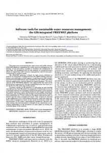

![[Download] [PDF] Oracle and Open Source: Tools and ... - Google Sites](https://m.moam.info/img/260x300/download-pdf-oracle-and-open-source-tools-and-goog_64789940097c4744708d02d0.jpg)


