Integrating Heterogeneous OO Schemas - Semantic Scholar

SCHEMA INTEGRATION JOURNAL OF INFORMATION SCIENCE AND ENGINEERING 16, 555-591 (2000)

555

Integrating Heterogeneous OO Schemas YANGJUN CHEN IPSI Institute, GMD GmbH 64293 Darmstadt, Germany E-mail: [email protected]

A key problem in providing enterprise-wide information is the integration of databases that have been independently developed. A major requirement is to accommodate heterogeneity and at the same time preserve the autonomy of component databases. This article addresses this problem and presents a strategy to integrate heterogeneous OO schemas. As compared to the existing methodologies, this approach integrates local schemas into a deduction-like global schema. In this way, more semantic relationships of component schemas can be captured, and more complete integration can be obtained. In addition, an efficient algorithm is proposed which can do the integration almost automatically, based on the correspondence assertions supplied by designers. This algorithm is efficient in the sense that the characteristics of assertions are utilized to avoid useless matchings. Keywords: federated databases, correspondence assertion, schema integration, derivation assertion, integration algorithm

1. INTRODUCTION With the advent of applications involving increased cooperation among systems, the development of methods for integrating the pre-existing databases has become important. The design of such global database systems must allow unified access to diverse and possibly heterogeneous database systems without subjecting them to conversion or major modifications [4, 7, 11, 18, 33]. One important step in integrating heterogeneous systems is to build a global schema from local ones, which is usually done in two phases: schema transformation and schema integration [1, 30]. By means of schema transformation, a local schema is transformed into an abstract one, e.g., an object-oriented schema [24, 25]. Then, all the local object-oriented schemas are integrated into a global one, thereby removing semantic conflicts caused by different perceptions of the same real world concepts. To eliminate semantic conflicts among the component databases, a set of correspondence assertions for declaring their semantic relationships has to be constructed by DBAs or by users. Normally, four set relationships between object classes, equivalence, inclusion, intersection, and exclusion, are defined so as to provide knowledge about correspondences that exist among the local schemas [35]. In this article, we will introduce a new assertion, the so-called derivation assertion, to accommodate more heterogeneities, which can not be treated using the existing methodologies (see [2, 10, 13, 22, 27, 35]). As an example, consider two local object-oriented schemas, S1 and S2. Assume that S1 contains two classes, parent and brother, and that S2 contains one class, uncle. A derivation assertion of the form S1(parent, brother) → S2 (uncle) can specify their corresponding semantic relationship clearly, which can not be Received December 17, 1998; revised April 1, 1999; accepted June 5, 1999. Communicated by Arbee L. P. Chen.

555

556

YANGJUN CHEN

established otherwise. We claim that this kind of assertion is necessary for the following reason. Imagine a query concerning uncle, submitted to the integrated schema from S1 and S2. If the above assertion is not specified, the query evaluation will not take schema S1 into account; thus, the answers to the query will not be correctly computed in the sense of cooperations. Some more complicated examples will be given later to show that derivation assertions can always be used to handle intricate semantic relationships. Recently, the problem of schema integration has been addressed extensively. In [35], the four semantic assertions mentioned above were used to declare semantic conflicts between two heterogeneous schemas. In addition, attention was paid to the path correspondence problem there. However, no formal method has been developed for this situation. In [13], another kind of path correspondences was introduced, with which more difficult semantic conflicts (like S1(Salary.Person) ~ S2(Salary.Salesmen.Person), indicating that Salary of Person from S1 and Salary of Salesmen from S2 are identical) can be tackled. However, no derivation relationships can be dealt with in this way, either. In fact, such a path correspondence can be declared using a combination of equivalence and inclusion. That is, we can declare S1(Person) ⊇ S2(Salesmen), thereby specifying that the attribute Salary of Person is equivalent to Salary of Salesmen. In [22], a hyperrelation approach was proposed, with which different attributes of relevant concepts (belonging to different local schemas) can be connected together. Similarly, no derivation problem is considered in this method. In [26], a formal method to describe schema equivalence was developed. It distinguishes between “unconditional” equivalence and the “conditional” equivalence, and also can not be used to declare the derivation relationship. A similar approach was described in [15], where the notion of a database “context” is used to specify conditionally equivalent concepts. In the other methods, such as those proposed in [2, 10, 27], derivation correspondence is not mentioned at all. To integrate relevant concepts connected by derivation assertions, however, the deductive approach should be employed, and a mechanism to do inferences should be developed to support such more complete global schemas. For this purpose, we simplify the data model proposed in [16] by replacing the concept of “object constructors” with that of “aggregation functions”, which is well-defined, extends predicate calculus and enriches the object-oriented model with deduction abilities. In this way, an object-oriented global schema can be equipped with an inference mechanism to capture more semantics. (More importantly, this concept can be easily implemented on the “Ontos” system [28] by using its aggregation functions. “Ontos” does not support the concept of object constructors; our system is built on “Ontos”.) As we will see later, the path problem proposed in [34, 35] can also be handled formally in our framework. In addition, autonomy is not violated since the “virtual” inferences (more exactely, rule evaluation; see Appendix B) are performed only at an abstract level and no extra requirements are placed on the local databases. On the other hand, the integration algorithm has not been studied extensively in previous work concerning federated databases. Although several approaches [33, 35] have been suggested, in terms of the given assertions, to integrate local schemas automatically, no effort has been made to optimize this process. That is, no analysis of correspondence assertions has been done to minimize redundant operations by using their characteristics. Furthermore, in [33, 35], only equivalence and inclusion assertions were considered by an integration process; ways to deal with the other kinds of assertions were not considered. In addition, approaches to integrating aggregation links as well as is-a links (paths) have not

SCHEMA INTEGRATION

557

been fully addressed up to now. In fact, these problems are not trivial, and some attention should be paid to them. To this end, we present a new algorithm for perfoming integration almost automatically while taking the assertion characteristics and link integrations into account to achieve high performance. The remainder of this article is organized as follows. Section 2 introduces the data model used in our system. In section 3, our system architecture is briefly outlined. Section 4 discusses the assertion set, through which the semantic correspondences between local schemas can be defined. In section 5, we give our integration principles. Section 6 is devoted to a integration algorithm. Finally, conclusions are set forth in section 7.

2. OBJECT MODEL As discussed in the introduction, we need a powerful data model to represent integrated schemas. One way to do this is to accommodate deduction with complex objects and object identities so that local databases can be integrated more fully into a deduction-like object-oriented schema. In the following, we will present an object model with well-defined semantics that equips complex objects with a deduction capability. This object model is used to represent the integrated information in our system. In fact, our model is a modification of those proposed in [16, 23]. First, in our model, the object identifiers can be referenced only through aggregation functions, rather than as attribute values as suggested in [16]. In addition, we implement the concept of object constructors developed in [16] as a combination of aggregation functions in a natural way. Further, due to the above modification, a rule in our model is simply a clause of the firstorder logic [20], and no extra complexity is assumed, as compared with the object constructors. On the other hand, the aggregation function is supported in the “Ontos” system [28], which is used as our platform. In our model, a schema is defined as a set of classes C. The type of a class C in C, denoted by type(C), is defined as: type(C) = , where ai represents an attribute name, typei ∈ {boolean, integer, real, character, string, date} ∪ type(C) and Aggj represents an aggregation function: type(C) → type(C') (C, C' ∈ C). Further, each aggregation function may be associated with a cardinality constraint ccj ∈ {[1:1], [1:n], [m:1], [m:n]} (j = 1, ..., k). For instance, a class Article may be of the type: type(Article) = , where ‘Published_in: Proceedings’ represents an aggregation function (aggregation relationship) Article → Proceedings, specifying the semantic relationship between domain class Article and range class Proceedings. Accordingly, an object (instance) of C is represented as a term (called the complex Oterm): ,

558

YANGJUN CHEN

where o is the object identifier, C is its class, ai’s are attribute names, vj’s are the corresponding values and each aggj represents an instance of Aggj. For example, an instance of class Article may be of the form: , where Published-in(.) takes ‘id_1’ as the input and returns a value, say ‘AI_Tool_91’, an object identifier of the class called Proceedings, which can be used to visit the corresponding object. In addition, when we refer to an object without considering its attribute values, we simply write instead of for convenience. The classes in an object database are organized into an inheritance hierarchy. We say that a class C is a subclass of another class C', denoted and , ¬ . In general, if we have a set of disjoint assertions, S1•Ai ∅ S2•Bj (i = 1, ..., n; j = 1, ..., m) with , for each i and j, and if IS(S1•A) ≡ IS(S2•B), then we can establish the following rule to integrate the relevant concepts: ∨ ...∨ ⇐ , ¬ , ..., ¬ . Alternatively, if there exists a specification about reverse aggregation functions, we can rewrite this principle in the following way: if S1 ∑ A ∆ S2 ∑ B then { if there exists S1 ∑ A ∑ aggA ¿ S2 ∑ B ∑ aggB then construct ‹ } and } ‹ , where ISagg ,agg is defined as follows: A

B

A

A

A

B

B

A

B

B

agg A ( x ) x ∈ IS( S1 • A); ISagg A , agg B ( x ) =  agg B ( x ) x ∈ IS( S2 • B).

(5) Integration principle for derivation assertions. As with the intersection assertion, for a derivation assertion, several virtual rules are constructed but in a more complex form. To this end, we first partition (manually) one derivation assertion into several smaller ones such that neither the attribute name nor the aggregation function appears more than once in an attribute correspondence or in an aggregation function correspondence. For example, assertions shown in Figs. 7(a) and (b) can be decomposed into the forms shown in Figs. 9 and 10, respectively. S1 ∑ car1 Æ S2 ∑ car2

S1 ∑ car1 Æ S2 ∑ car2

value correspondence of attributes in S1: no constrains

value correspondence of attributes in S1: no constraints



attribute correspodence:


S1 ∑ car1 ∑ time ∫ S2 ∑ car2 ∑ time

∑∑∑


S1 ∑ car1 ∑ car-name « S2 ∑ car2 ∑ {‘car-name1’}

S1 ∑ car1 ∑ car-name « S2 ∑ car2 ∑ {‘car-namen’}

S1 ∑ car1 ∑ price « S2 ∑ car2 ∑ car-name1

S1 ∑ car1 ∑ price « S2 ∑ car2 ∑ car-namen

Fig. 9. Decomposed derivation assertions for S1 ∑ car1 Æ S2 ∑ car2. S2 ∑ car2 Æ S1 ∑ car1

S2 ∑ car2 Æ S1 ∑ car1








∑∑∑

S2 ∑ car2 ∑ car-name1 Õ S1 ∑ car1 ∑ price with S1 ∑ car1 ∑ car-name = car-name1 (a)

S2 ∑ car2 ∑ time ∫ S1 ∑ car1 ∑ time S2 ∑ car2 ∑ car-namen Õ S1 ∑ car1 ∑ price with S1 ∑ car1 ∑ car-name = car-namen (b)

Fig. 10. Decomposed derivation assertions for S2 ∑ car2 Æ S1 ∑ car1.

572

YANGJUN CHEN

Then, we construct a graph G (called assertion graph) for each decomposed derivation assertion of the form S1(A1, A2, ..., An) → S2•B. In the graph, there is a node for each “path” refering to an element in some class (see Definition 3.1) and an edge between nodes patha and pathb iff patha rel pathb with rel ∈ {=, ∈, ⊆} is specified. For instance, for the assertion shown in Example 3, we can construct the graph shown in Fig. 11(a). S2 • uncle :

S1(parent, brother)

S2 • car2

S1 • car1 : y1

parent • Pssn#

x1

S1 • brother • Bssn#

x2

brother • brothers

S2 • uncle • Ussn#

S1 • car1 • time

S2 • car2 • time

S2 • car2-name1

y2

S1 • car1 • price y3

S1 • car1 • car2-name1 S1 • parent • children

x3 S2 • uncle • niece_nephew

p p: S1 • car1 • car-name = car-name1

(b)

(a)

Fig. 11. Assertion graph and hyperedges.

The key step in constructing a virtual rule is to establish the relationships among the O-terms of the rule to be constructed through variables as in Artificial Intelligence. (More exactly, specify variables as in parent(x, y), brother(z, y) → uncle(x, z).) For this purpose, we mark the nodes of G in the following way: (1) Each connected subgraph of G is marked using a different variable as shown in Fig. 11(a). For example, the connected subgraph consisting of only one edge (parent•Pssn#, brother•brothers) is marked x1. (2) For each predicate p(path1, ..., pathm) appearing in the assertion, we construct a hyperedge he(p), representing the set containing nodes path1, ..., and pathm. For example, in the graph associated with the assertion shown in Fig. 10(a), we have a hyperedge for the predicate S1•car1•car-name = car-name1 (see Fig. 11(b) for an example, in which the hyperedge is marked p.) Note that, here, car-name1 is a constant, and ‘= car-name1’ can be considered to be a predicate name. Then, ‘S1•car1•car-name = car-name1’ is a unary predicate. (We also note that the isolated node “S1•car1•car-name” is considered to be a connected subgraph, which is marked y3.) The goal of the assertion graph is to facilitate the generation of derivation rules. Given a derivation assertion of the form S1(A1, A2, ..., An) → S2•B, what we want is to establish a rule of the form B' ⇐ A1', A2', ..., An', p1, ..., pl, where B' and An' (i = 1, ..., n) are O-terms and pj (j = 1, ..., l) are normal predicates. Intuitively, B' corresponds to B, Ai' to Ai and pj to the predicates appearing in the assertion. They are logically linked together through shared attribute variables and object variables. We first define the following concepts. Definition 5.1 A reverse substitution θ is a finite set of the form {c1/x1, ..., cn/xn}, where each xi is a variable, each ci is a constant or a variable and c1, ..., cn are distinct. Each element ci/xi is called a binding for ci.

SCHEMA INTEGRATION

573

This concept can be thought of as a reverse operation of the substitution concept defined in [29]. In fact, we are performing a process which is just the reverse of rule evaluation in logic programming, by means of which variables are instantiated. But in a reverse substitution, a constant (or a variable) will be replaced with a variable. Definition 5.2 Let θ = {c1/x1, ..., cn/xn} be a reverse substitution, and let A be an O-term, a constant or a variable. Then, Aθ is an O-term (or a variable) obtained from A by simultaneously replacing each occurrence of ci in A with the variable xi (i = 1, ..., n). As an example, consider O-term B = . Let θ = {x/x2, y/x3}. Then, Bθ = . Note that in this example, both x and y are typed variables for strings. If S = {A1, A2, ..., An} is a finite set of O-terms, constants and variables, and if θ is a reverse substitution, then Sθ denotes the set {A1θ, A2θ, ..., Anθ}. Definition 5.3 Let θ = {c1/x1, ..., cn/xn} and δ = {d1/y1, ..., dm/ym} be reverse substitutions. Then, the composition θδ of θ and δ is the reverse substitution obtained from the set. {c1/x1δ, ..., cn/xnδ, d1/y1, ..., dm/ym} by deleting any binding ci/xiδ for which ci = xiδ and deleting any binding dj/yj for which dj ∈ {c1, ..., cn}. For a given derivation assertion, the relevant reverse substitutions can be produced in terms of its assertion graph G. According to the two different variable-marking approaches, we have two methods we can use to produce reverse substitutions: (i) Consider a connected subgraph Gs of G. Assume that Gs is marked using xs. Let {v1, ..., vt} be the node set of Gs. Then, each vq may be of the form C•ai•aij•aijk ... •“aij...hl...s” or of the form C•ai•aij•aijk ...•aij...hl...s (see Definition 4.1). If vq is of the form C•ai•aij•aijk ...•“aij...hl...s”, then construct a binding bq = C•ai•aij•aijk ...•“aij...hl... s”/xs. If vq is of the form C•ai•aij•aijk ...•aij...hl...s , then construct a binding bq = x/xs, where C•ai•aij•aijk ...•aij...hl...s: x is an attribute descriptor in the corresponding Oterm. In this way, we can produce a reverse substitution θs = {b1, ..., bq, ..., bt} for Gs. (ii) Let he(p) be a hyperedge containing nodes u1, ..., um, where p is a predicate appearing in the assertion. Let bq = c/x be the binding generated as described above for uq (q = 1, ..., m). If c is a variable, let bq' be a/x, where a:c is an attribute descriptor in the corresponding O-term. Otherwise, let bq' be bq. Then, the reverse substitution for the predicate p is the composition {b1'}...{bq'}...{bm'}. (Note that each {bq'} is a reverse substitution.) Based on the above discussion, the integration principle for derivation assertion can be summarized as follows: if S1 (A1, A2, ..., An) ÆS2 ∑ B then {construct an assertion graph G for it; mark each connected subgraph Gj of G using xj;

574

YANGJUN CHEN

construct a hyperedge for each predicate pi appearing in the assertion; for each Gj do generate reverse substitution qj; for each hyperedge he(pi) do generate reverse substitution di; generate a derivation rule of the form: Bq1...qj... ‹ {A1, A2,...,An}q1...qj, {p1,...,pi...} d1... di... } Example 9. Consider the derivation assertion given in Example 3. Its assertion graph can be constructed as shown in Fig. 11(a). Assume that the O-terms of the three classes are B = , A1 = and A2 = . Then, from that assertion graph, three reverse substitutions can be produced: θ1 = {z/x1, w/x1}, θ2 = {v/x2, x/x2} and θ3 = {u/ x3, y/x3}. According to the above principle, an inference rule of the following form will be constructed: Bq1q2q3‹ {A1, A2} q1q2q3 fl ‹ , . Example 10. Applying this principle to the decomposed assertions shown in Fig. 10, we can establish a set of rules as follows: ‹ , y2 = car-name1 ...

‹ , y2 = car-namen. We need only to consider assertion shown in Fig. 10(a), for which a graph as shown in Fig. 11(b) can be constructed. Assume that the O-terms of class car1 and car2 are of the forms B = , and A = , respectively. Then, from that assertion graph, four reverse substitutions can be generated: θ1 = {x/y1, u/y1}, θ2 = {v/y2, z/y2}, θ3 = {y/y3} and δ = {car-name/y3}. The first three are produced as its connected subgraphs while the last one is established according to the hyperedge in it. Let p denote the predicate S1•car1•car-name = car-name1. Then, the first rule of the above set can be built as follows: Bq1q2q3 ‹ Aq1q2q3, pd fl ‹ , y2 = car-name1.

SCHEMA INTEGRATION

575

Example 11. Given assertions shown in Figs. 6(b) and (c), the following two inference rules can be constructed based on the above principle: ‹ , ‹ . If the attribute book in the class Author and the attribute author in the class Book are defined as aggregation functions, then we can generate the following two simpler rules using the above principle with a bit of modification: ‹ ‹ . As in a deductive database, the generated rules should be checked to see whether they are well-defined, safe, or domain independent and allowed in the presence of negated body predicates [8]. (6) Integration principle for is-a and aggregation links. As for an is-a link is_a(A, A') in a local schema S1, let us consider the pair of the form (B, B') in another schema S2, which satisfies the following conditions: - B and B' are connected with an is-a path, i.e., a path of the form: B ← ... ← B'; - IS(S1•A') ≡ IS(S2•B') and IS(S1•A) ≡ IS(S2•B). Then, if we insert any local is-a link into the integrated schema S (in fact, using our integration algorithm, this simple strategy can be employed), we will have some subgraphs of the forms as shown in Figs. 12(a) and (b) in the integrated schema. IS A’B’

IS A’B’ *

*

IS AB IS AB (a)

(b)

Fig. 12. Redundant is-a links which may exist in an integrated schema.

Therefore, for the subgraph shown in Fig. 12(a), only one of the two links should be inserted while for the subgraph shown in Fig. 12(b), the link indicated by * should not be inserted. This principle can be formally represented as follows: if IS(S1∑A') ∫ IS(S2∑B'), IS(S1∑A) ∫ IS(S2∑B), (is_a(A, A') ⁄ is_a(B, B')) then insert is_a(ISAB, ISA’B’) into S.

576

YANGJUN CHEN

if IS(S1∑A') ∫ IS(S2∑B'), IS(S1∑A) ∫ IS(S2∑B), is_a(A, A'), is_a(B, B1), is_a(B1, B2),..., is_a (Bn, B') then insert is_a(ISAB, IS(B1)), is_a(IS(B1), IS(B2)),..., is_a(IS(Bn), ISA’B’) into S. For the aggregation links, we consider only links of the form agg(B, B') and agg(A, A') with IS(S1•A') δ IS(S2•B') and IS(S1•A) δ IS(S2•B) (δ ∈ {≡, ∩}). In these cases, the cardinality constraints associated with them should be integrated. To this end, consider the simple constraint lattice shown in Fig. 13(a).

[n : m] [1 : m]

[n : 1]

[1 : 1]

(a) [m : n] [m: md_n]

[n : 1]

[n: md_1]

[md_1: n]

[md_1: md_n]

[md_1: 1]

[md_m: n] [md_m: md_n] [md_n: 1] [md_n: md_1]

[1 : n] [1: md_n]

[1:

[1: md_1]

[md_1: md_1]

(b)

Fig. 13. Constraint lattices.

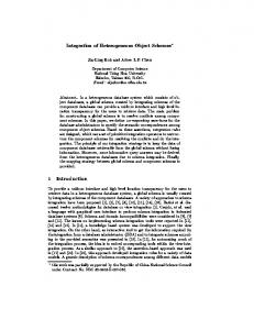
Based on this constraint lattice, the principle for resolving the constraint conflicts can be described as follows: if Agg(A', A) with cc1, Agg(B', B) with cc2 then {insert Agg(ISA'B', ISA'B') with lcs(cc1, cc2) into S}, where lcs(cc1, cc2) represents the ‘least common super-node’ of cc1 and cc2. For example, [n : m] is lcs([1: m], [n : 1]) while [n : 1] is lcs([1: 1], [n : 1]). In addition, a node is considered to be the least common super-node of itself. This idea can be generalized for more complicated cases. Consider, for example, the cardinality constraint of the so-called “mandatory n to 1”, denoted [md_n : 1], which can be used to specify the situation where the participation is total (mandatory) and the mapping is “n to 1”. If some constraints like this are involved, we can establish a constraint lattice as shown in Fig. 13 (b) to make the above principle implementable. This lattice reflects a relaxation strategy of the cardinality constraints. If a constraint conflict is encountered, we can resolve it by loosening the local constraints along the lattice from bottom-up, which is least loosened.

SCHEMA INTEGRATION

577

6. CONTROLLING THE INTEGRATION PROCESS In this section, we will discuss our integration algorithm. This algorithm generates almost automatically an integrated schema from two local object-oriented ones based on their correspondence assertions declared by users. Only in very difficult situations is human interference needed. (See the discussion in 6.1.) The algorithm is efficient compared to that proposed in [33] since the semantics of local schemas are used to avoid the need to check useless pairs of concepts. More importantly, a semantically clear integrated schema can be generated by avoiding redundant is-a links. In subsection 6.1, we specify the main part of our algorithm in detail. In subsection 6.2, we discuss how to integrate links. Finally, the correctness and time complexity of the algorithm are considered in subsection 6.3. 6.1 Integration Algorithm Notice that in our methodology, any local schema will be transformed into an objectoriented one before the integration process is performed. Consequently, a local schema can be viewed as a graph consisting of a set of object classes connected by is-a links, aggregation links or semantic constraints. Accordingly, the input of the following algorithm for controlling the integration process consists of two graphs (with each representing a local schema) and a set of assertions. In the following, we will not consider the principles for integrating links. We will postpone the relevant discussion concerning link integration to subsection 6.2. In addition, to simplify the explanation, we will assume that each graph has a start node and will be S1:

S2:

Fig. 14. Illustration of input graphs.

traversed only along is-a links. If an input graph does not have such a node, we construct a virtual one for it, and for each of those nodes which have no parent nodes in the original graph, we draw a meaningless edge from it to the virtual start node. Then, the input graphs of the algorithm can be illustrated as shown in Fig. 14, where each node corresponds to a class and each arc corresponds to an is-a or an aggregation link. To perform the integration, a naive algorithm will check, for example, all nodes in S2 for each node in S1 to see whether some integration should be done on the corresponding concepts. If each local schema contains O(n) nodes, then, including the time spent on the integration operations, the time complexity of a naive algorithm will be larger than O(n2). Below is a naive algorithm which uses a breadth-first-search but works in a different way from that proposed in [33]. Algorithm naive_schema_integration input: S1, s1; S2, s2; (*s1 and s2 represent the start nodes of S1 and S2, respectively.*) output: S (*S represents the integrated schema.*)

578

YANGJUN CHEN

begin 1 Q: = (s1, s2); (*Q is a queue structure used to control breadth-first search*) 2 while Q is not empty do 3 { (N1, N2):= pop(Q); (*take the top element of Q*) 4 let N11,...,N1k be child nodes of N1; 5 let N21,...,N2m be child nodes of N2; 6 put all the pairs of the form (N1i, N2j), (N1, N2j) or (Nli, N2) (i=1,..., k; j=1,..., m) into Q; 7 do the integration according to the assertion between N1 and N2; } end In this algorithm, a queue structure Q is used to control a breadth-first search of two input graphs. Each element in Q is a pair (N, N'), where N is a node in S1 and N' a node in S2. In each iteration, the top pair (a, b) of Q will be checked, and the corresponding integration operation will be performed as described in section 5. Simultaneously, all the pairs of the form (a', b') are put into Q, and are checked in the subsequent iterations, where a' is a or an a's child node and b' is b or a b's child node. We note that this control mechanism is quite different from that proposed in [33]. There, traversal of the two input graphs is completely separated. That is, traversal is performed in one of the two input graphs, say S1. Then, for each node in S1, the entire S2 is searched. In contrast, in the above algorithm, these two processes are integrated together, based on which a lot of optimization (which will be discussed below) can be realized without difficulty. More importantly, the integration principle for inclusion of assertions (for which links will be generated) can be elegantly handled by integrating a depth-first traversal into this algorithm. First, we will consider the possibility of optimization by analyzing the characteristics of correspondence assertions. The following observations are important. S2 :

S1 : N N

N

1

N

11

N

12

N

13

2

N

21

N

22

N

2

23

Fig. 15. Two simple input graphs.

1. Consider the two simple graphs shown in Fig. 15. If they are the input graphs and N1 ≡ N2 is an assertion in the assertion set, then the pairs pa1 = {(N1, N21), (N1, N22), (N1, N23), (N1, N24)} and pa2 = {(N11, N2), (N12, N2), (N13, N2)} needn’t be checked for the following reason. Consider any N ∈ {N21, N22, N23, N24}. Then, from N1 ≡ N2 and is_a(N, N2), we know immediately that is_a(IS(N), IS(N1)) holds. That is, the semantic correspondences between each pair of pa1 can be derived. The same analysis applies to all pairs of pa2. 2. Consider Fig. 15 again. If N1 ⊆ N2 is specified, then all the pairs of pa2 needn’t be checked either since for any N ∈ {N11, N12, N13} is_a(IS(N), IS(N2)) can be decided from the relationships N1 ⊆ N2 and is_a(N, N1) without doing any checking. However, all the pairs of pa1 have to be checked since in this case, nothing can be inferred from N1 ⊆ N2

579

SCHEMA INTEGRATION

and the other known is-a relationships. Similarly, if N1 ⊇ N2 is specified, then pa1 should be but pa2 needn’t be checked. In addition, this observation can be generalized to ‘is-a’ paths. That is, if B1 ← B2 ← ... ← Bk is a path in S2, S1(A) ⊆ S2(Bk) holds and A1 is a subclass of A, then the relationships S1(A1) ⊆ S2(Bk), ..., S1(A1) ⊆ S2(B1) can be inferred. Thus, the corresponding pairs needn’t be checked. 3. If N1 ∅ N2 or a derivation assertion involving N1, and if N2 is specified, then we will check neither pa1 nor pa2. This is because, in this case, no clear semantic relationships between each pair of pa1 and pa2 can be defined. For example, if S1(man) ∅ S2(woman) is defined and S1(man_student) is declared to be a subclass of S1(man), then one will tend not to give an assertion to specify the semantic relationship between S1(man_student) and S2 (woman). As another example, consider the assertion S2(parent, brother) → S1(uncle). One might not specify an assertion between S2(old-brother) and S1(uncle), either. Therefore, ignoring such pairs is reasonable. Of course, it is possible that some assertions between such pairs may be specified. But we believe that ignoring such assertions will not damage the semantics of the integrated schema - a theme in forthcoming research. Alternatively, if such pairs exist, we may, for the purpose of safety, inform the user that something is strange, and ask her or him whether the assertion is correct or a mistake. (This is the only case where user interference is required.) 4. If N1 ∩ N2 is specified, then both pa1 and pa2 should be checked. This is because, from N1 ∩ N2, we can not derive anything about the relationship among N1_(part of N1 which does not belong to N2) and the child nodes of N2. (The same analysis applies to N2_ and the child nodes of N1.) Further, in the case where no assertion between N1 and N2 is given, the pairs of pa1 and pa2 should be checked completely. Obviously, in order to speed up the above algorithm, lines 6 and 7 in the algorithm have to be changed so that only some of pairs are put into the queue Q based on different correspondence assertions. In addition, a depth-first-search should be integrated to search is-a paths so that the integration principles for inclusions can be fully implemented in a convenient way. Further, to avoid any redundant operations during graph traversal and to implement the integration principle for inclusion assertions uniformly, we introduce a labelling technique and a mechanism for label inheritance used to mark the corresponding pairs, which needn’t be checked during graph traversal. See the following Fig. 16.

S1

S2 :

:

subset

N1

l1

N2

l1 subset b1

c2 l1.l2

d2

h2

l 2 b2

l1

subset i2

e1

l2

c2

l2

l1.l2 j2

d2

l1

l2

k2

l1

e2 f2

Fig. 16. Illustration of node labelling.

580

YANGJUN CHEN

In this diagram, if N1 ⊆ N2 is specified, we will use a depth-first search to traverse the subgraph rooted at N2, thereby labelling any path of the form P = N2 ← ... ← N (starting at N2) with the following properties: (i) for any node v (≠ N) on P, N1 ⊆ v is specified or no assertion between N1 and v is defined; (ii) N1 ≡ N, or N1 ⊆ N but for any descendent node Nc of N, neither N1 ≡ Nc nor N1 ⊆ Nc is defined. Assume that the path N2 ← b2 ← c2← d2 ← e2 in the diagram shown in Fig. 16 is one such path. Then, during depth-first traversal, we will mark all the nodes on the path with a label, say l1, to indicate that these nodes should not be checked against any node in the subgraph rooted at N1. To do this, N1 will also be labelled with l1, and it will further be inherited by all N1’s child nodes. Then, in the subsequent traversal, we can use l1 to avoid checks of b1, c1 and d1 against any node labelled with l1 in S2. Similarly, e1 will not be checked against these nodes (in S2) either, in terms of label l1 inherited from b1. During graph traversal, some other paths will be marked (with different labels) for the same reason. For example, the path h2 ← i2← j2 shown in the above diagram may be labelled with l2 if b1 ⊆ h2, b1 ⊆ i2, b1 ⊆ c2 but b1 ⊆ k2, θ ∈ {→, ∅, ∩}. Then, the label for b1 will be changed to l1 ⋅ l2 to indicate that all the nodes in the subgraph rooted at b1 will not be checked against any node labelled with l1 or l2 in S2. (According to the inheritance mechanism, all the child nodes of b1 will also possess l1 ⋅ l2.) In general, if a node in S1 is labelled with l1 ⋅ l2 ⋅ ... ⋅ lk, it should not be checked against any node labelled with l1 or l2 or ... or lk in S2. Similarly, if a node in S2 is labelled with l1’ ⋅ l2’ ⋅ ... ⋅ lj’ besides any label of the form li, it should not be checked against any node labelled with l1’ or l2’ or ... or lj’ in S1. Below, we will show that each node in S1 and S2 will be labelled with a pair of label sequences to implement this duality. The following algorithm (named schema_integration) is mainly based on a combination of breadth-first and depth-first search. By means of breadth-first search, a control similar to naive_schema_integration is performed, but with label inheritance and some optimization. By mean of depth-first search, the above labelling technique is implemented. To control the breadth-first search, a queue structure Sb is used to record node pairs of the form (N1, N2), whose semantic relationship is to be checked. Further, a stack structure Sd is utilized to control the local depth-first search (in S1 or in S2) when a pair with assertion ⊆ (or ⊇) is encountered during breadth-first traversal. (See lines 11 and 18; depth-first search is done by calling path_labelling; see below.) Essentially, the main control is done in lines 3-6 of the following algorithm. Let (s1, s2) be the pair being considered. Assume that s1 has child nodes N11, ..., N1k, and that s2 has child nodes N21, ..., N2m. Then, all the pairs of the form (N1i, N2j) (i = 1, ..., k; j = 1, ..., m) will be put into Sb for subsequent checks. Further, in terms of the assertion between s1 and s2, pairs of the form (s1, N2j) or (N1i, s2) (i = 1, ..., k; j = 1, ..., m) may not be put into Sb since their semantic relationships may be derived. (See the discussion above again to understand lines 16, 23, 31, and 33-35.) Additionally, slightly deviating from the labelling technique discussed above, each node N of S1 and S2 is dynamically associated with a pair of label sequences, , instead of only a label sequence. (We discuss this technique in this way so that the

SCHEMA INTEGRATION

581

main idea behind the mechanism can be well understood.) Here, l1 ⋅ ...⋅ ln are called the labels of N, denoted labels(N), representing labels obtained during depth-first search while l1’⋅ ...⋅ lm’ are the labels obtained through inheritance, called the inherited labels of N and denoted inherited-labels(N). Therefore, for a current node Ni, inherited-labels(Ni) = l1’⋅ ... ⋅ lm’ indicates that if a node Nj (in another graph) possesses a label pair with labels(Nj) = l1”⋅ ...⋅ lk” such that {l1”, ..., lk”} ∩ {l1’, ..., lm’} is not empty, then Nj should not be checked against Ni (see line 7.). When node N1 in S1 meets N2 in S2 the first time, and when for them N1 ⊆ N2 is specified, depth-first-search will be executed to traverse the subgraph rooted at N2. By this process, any node N with the properties i) and ii) shown above will be labelled, and some integration operations over N1 and the nodes encountered during traversal will be performed. Finally, we assume that each node of S1 and S2 is initially associated with an empty label pair: < , >. Algorithm schema_integration ( (* breadth-first search*) input: S1, s1; S2, s2; (*s1 and s2 represent the start nodes of S1 and S2, respectively.*) output: S (*S represents the integrated schema.*) begin 1 l: =0; (*l is used to label paths during depth-first search.*) 2 Sb: = (s1, s2); 3 while Sb is not empty do 4 {(N1, N2): =pop(Sb); 5 let N11, ..., N1k be child nodes of N1; let N21, ..., N2m be child nodes of N2; 6 put all the pairs of the form (Nli, N2j) (i=1, ..., k; j=1, ...,m) into Sb; 7 if inherited-labels (N1) « labels (N2) = f Ÿ labels (N1) « inherited-labels (N2) = f then 8 {switch (N1 q N2) { 9 case N1 ∫ N2: put N = merging (N1, N2) into S; 10 let M11, ..., M1i be brother nodes of N1; let M21,..., M2j be brother nodes of N2; remove the pairs of the form (N1, M2j) or (M1i, N2) from Sb; break; 11 case N1 Õ N2: call path_labelling (N1, S2, N2, l); (*Algorithm path_labelling is given below.*) 12 let l’ be the returned label of path_labelling; 13 inherited-labels (N1): = labels (N1). l’; 14 for each child node Nli of N1 do 15 inherited-labels (Nli):= inherited-labels (N1); 16 put all the pairs of the form (N1, N2i) into Sb; 17 break; 18 case N1 N2: call path_labelling (N2, S1, N1, l); 19 let l’ be the returned label of path_labelling; 20 inherited-labels (N2):= inherited-labels (N2). l’; 21 for each child node N2i of N1 do 22 inherited-labels (N2j):= inherited-labels (N2); 23 put all the pairs of the form (N1i, N2) into Sb;

582

YANGJUN CHEN

24 break; 25 case N1 ∆ N2: construct the corresponding rules in terms of Principle 4; 26 case N1 and N2 involved in a derivation assertion: 27 construct the corresponding rules in terms of Principle 5; 28 break; 29 case N1 « N2: insert IS(N1) and IS(N2) into S; 30 construct rules defining IS(N1_), IS(N2_) and ISN1N2 based Principle 3; 31 put all the pairs of the form (N1, N2j) and (N1i, N2) into Sb; 32 break 33 default: put all the pairs of the form (N1, N2j) and (N1i, N2) into Sb;}} 34 else if inherited-labels(N1) « lables (N2) π f then put all the pairs of the form (N1, N2j) into Sb; 35 else put all the pairs of the form (N1i, N2) into Sb; } end In the above algorithm, one of seven cases, N1 ≡ N2, N1 ⊆ N2, N2 ⊆ N1, N1 ∅ N2, “N1 and N2 involved in a derivation assertion”, N1 ∩ N2, and “no assertion specified between N1 and N2” is handled in each step of breadth-first traversal. If N1 ≡ N2, then only the pairs of the form (N1i, N2j) are put into Sb. In addition, all the pairs of the form (N1, M2j) or (M1i, N2) (where M1i and M2j represent the brother nodes of N1 and N2, respectively) should be removed from Sb since the relationship between N1 (N2) and M2j (M1i) is the same as the local relationship between N2 (N1) and M2j (M1i). If N1 ⊆ N2, then depth-first search (by calling path_labelling; see below) will be performed over a subgraph of S2 (rooted at N2), in which the label sequence of each node P will be lengthened with a new label (see line 1 of path_labelling) if it is reached by mean of depth-first traversal and satisfies N1 ⊆ P. Furthermore, the corresponding integration operation will be performed whenever the appropriate node of S2 is encountered during depth-first traversal. (See lines 10-12, 13-17, 19-25 of path_labelling.) The new label will be returned from path_labelling, and N1’s inherited label will also be lengthened with it. Then, this new inherited label will be transferred to all its child nodes to execute label inheritance. A similar description applies for the case N2 ⊆ N1. In the fourth, fifth and sixth cases, the corresponding integration operations will be performed without any optimization. If no assertion is specified for N1 and N2, nothing will be done; traversal continues. Finally, we note that the labels are checked in lines 7 and 34 to avoid any useless matching. As mentioned earlier, depth-first-search should be employed to tackle the integration principle for the inclusion assertion, by means of which the is-a paths have to be searched ahead of the breadth-first-search process. On the one hand, some integrated is-a links should be created according to this principle. On the other hand, we should avoid any redundant traversal caused by the combination of these two orthogonal search strategies. To this end, we label the paths with the properties discussed above during depth-first search. Then, this label will be returned to the breadth-first-search process to avoid useless checks. In addition, to cope with cases where no assertions are defined at all for some nodes (classes), we denote these nodes using a special symbol, e.g., ‘*’, during local depth-first-search. Then, based on a backtracking mechanism, the integration principle for the inclusion assertion can be implemented as discussed in the previous section.

SCHEMA INTEGRATION

583

Algorithm path_labelling (*depth-first search*) input: N1, T, N2, l output: l (*l will be changed during the algorithm and used as the otput.*) begin 1 l:= l+1; 2 Sd:= N2; 3 while Sd is not empty do 4 {V:= pop(Sd); 5 switch (N1 q V) { 6 case N1 Õ V: labels (V): = labels (V). l; 7 let V1, ..., Vk be child nodes of V; 8 put all the nodes Vi (i = 1,..., k) into Sd; (*go deeper into the graph*) 9 break; 10 case N1 ∫ V: labels (V):= lables (V).l; 11 put N = merging (N1, V) into S; 12 break; (* the remaining part of the current path will no longer be searched.*) 13 case q Œ {Æ, ∆, }: let Uk ¨ Uk-1*¨ Uk-2*...¨ U1* ¨ V) be an is-a path in T such that 14 all nodes but Uk and V on it are denoted by*; 15 for all Uj* (j = 1,..., k-1) do 16 labels (Uj*): = labels (Uj*)/l; (*undo the invalid labels; i.e., in the subsequent traversal, such nodes should not be prevented from being checked against any node in the subgrah rooted at N1.*) 17 insert is_a (IS(N1), IS(Uk)) into S; (*N1 Õ Uk must be specified; based on Fig. 8(b), an is-a link should be generated.*) 18 break; 19 default: mark V with*; 20 if V has child nodes, then put all child nodes into Sd (*go deeper into the graph*) 21 else {let Uk ¨ Uk-1* ¨Uk-2*...¨U1*¨V) be an is-a path in T such that all 22 nodes but Uk and V on it are denoted by*; 23 for all Uj* (j = 1,..., k-1) do 24 lables (Uj*): = lables (Uj*)/l; (*undo the invalid labels*) 25 insert is_a (IS(N1), IS(Uk)) into S;}} } end In the above algorithm, any path rooted at N2 is traversed until a node N with one of the following properties is encountered: (1) N1 ≡ N; (2) N1 θ N with θ ∈ {→, ∅, ∩, ⊇}; (3) N is an end node. In the first case (see lines 10-12), we generate an integrated class for N1 and N and the remainder of the corresponding path will not be searched. In the second and third cases (see lines 13-18 and lines 19-25, respectively), we backtrack (along the corresponding path) to the first node N’ which is not denoted by *. In terms of the characteristics of the algorithm, we know that N1 ⊆ N’ must be specified. Then, an is-a link will be created just as Principle 2. In Appendix A, we trace a sample integration process to demonstrate how the algorithms work.

584

YANGJUN CHEN

6.2 More About Link Integration In the algorithm presented above, link integration is not considered at all. In our implementation, each local link is implicitly taken as a link in the integrated schema in this procedure. Consequently, in an integrated schema generated by the above algorithms, some subgraphs as shown in Fig. 12 may exist. Based on Principle 6, the edge denoted by * in such graphs should be removed. Further, for the aggregation links, we should replace the corresponding semantic constraints with their ‘least common super-constraint’ w.r.t. the constraint lattice shown in Fig. 13. To address these problems, we modify the above algorithms a bit as follows. First, we mark each node A (using a special symbol), for which an equivalence assertion is specified. Then, we check its father node B to see whether it has already been marked. If so, we further check B’s counterpart C to see whether A’s counterpart D is a child node of C. (See Fig. 17(a) for an illustration.) In this way, we can easily identify the subgraphs of the form shown in Fig. 12(a). C

B

C

B subset

A

D (a)

N2

N1 A (b)

Fig. 17. Illustration of link integration.

In the case of is-a links, we remove one of the two edges. Otherwise, we integrate the two aggregation links into one link with the semantic constraint being its lcs. Of course, the aggregation links to be integrated must have similar meaning, and their relationship must have been declared. (See Principle 6.) The same technique applies to subgraphs of the form shown in Fig. 12(b). Consider algorithm path_labelling once again. If the returned value of this algorithm is not a label, but rather a pair consisting of a label and a node A, for which an equivalence assertion is specified (see lines 9-11 in path_labelling), and if the current call of path_labelling is of the form path_labelling (N1, S2, N2, l), then we need to check N2’s father node B to see whether it has been marked. If it has been marked, then we check B’s counterpart C to see whether N1 is a child node of C. (See Fig. 17(b) for an illustration). In this way, this kind of subgraph can also be identified without difficulty. 6.3 Correctness and Time Complexity of the Refined Integration Algorithm The correctness of the refined integration algorithm can be directly derived from the discussion given just before the description of that algorithm in subsection 6.2. This is because the difference between the algorithms naive-schema-integration and schema-integration lies only in the fact that by the latter some pairs are not checked. However, based

SCHEMA INTEGRATION

585

on that discussion, the removed pairs really do not need to be considered, and their semantic relationships are included eventually in the integrated schema; or all the pairs are checked explicitly or implicitly using schema-integration. We distinguish among three kinds of pairs (N1, N2), where N1 ∈ S1 and N2 ∈ S2: (1) those pairs that are really checked during the execution of schema-integration; (2) those pairs of the form (N1, N2) with the following properties: (i) there exists an N ∈ S1 (N ∈ S2) such that N is an ancestor of N1 (N2) and (ii) N ≡ N2 (N ≡ N1) holds; (3) those pairs (N1, N2) with N1 being labelled using and N2 being labelled using such that {l1, ..., ln} ∩ {l1”’, ..., lk’”} = φ or {l1’⋅ ...⋅ lm’}∩ {l1” ⋅ ...⋅ li”} = φ. From lines 9-10 of schema-integration, we can see that the second kind of pair will not be checked. However, it really needn’t be checked since the semantic relationship between each pair of this kind can be directly derived. From line 7, if {l1, ..., ln} ∩ {l1”’, ..., lk’”} is not empty or {l1’⋅ ...⋅ lm’}∩ {l1” ⋅ ...⋅ li”} is not empty, then the corresponding pair (N1, N2) will not be checked, either. This is because their semantic relationship can also be inferred according to the integration principle for inclusion and the inclusion relationship between some of their ancestors. From schema-integration, we can see that no other pairs are ignored. Therefore, we claim that all the pairs are checked explicitly or implicitly, which guarantees the correctness of the algorithm. To simplify the time complexity analysis, we assume a simple setting where both S1 and S2 have tree structures and each concept from S1 has exactly one equivalent counterpart from S2. Further, we assume that both S1 and S2 have the same height h. We denote the average number of pairs (N1, N2) (N1 ∈ S1, N2 ∈ S2) checked during the process as Ωh. Let d be the average degree (the number of edges incident to a node) of the tree corresponding to S1. Then, we have the following recurrence relations: Ωh = Ω h −1

n 1 ⋅ (1 + d ⋅ Ω h −1 + 0 ), d 2 n 1 = ⋅ (1 + d ⋅ Ω h − 2 + 1 ), d 2

LL Ω h−i =

n 1 ⋅ (1 + d ⋅ Ω h − i + i ), d 2

LL

The first recurrence relation is obtained as follows. We will consider two “extreme” cases. The first case is where the roots of S1 and S2 match. In this case, the average number of the pairs to be checked should be 1 + d⋅Ωh-1. The second case is where the root of S1 matches some leaf node of S2. In this case, since the rest of the nodes of S1 needn’t be checked against S2, the total number of pairs checked is on the order O(n). Therefore, the 1 n average number of the pairs to be checked is ⋅ (1 + d ⋅ Ω h −1 + 0 ) . Expanding the above 2 d recurrence relations, we can derive Ωh = O(n).

586

YANGJUN CHEN

7. CONCLUSIONS In this paper, a new strategy is presented for integrating local OO schemas into a deduction-like one. On the one hand, a new correspondence assertion (derivation assertion) has been introduced to accommodate more heterogeneities which can not be handled by any existing method. On the other hand, a more powerful object model has been discussed, which enriches the object-oriented data model with deductive abilities. In this way, not only can the derivation assertion be tackled without difficulty, but some other complex semantic relationships, such as the ‘path’ concept proposed in [35] and role-consistency addressed in [32], can be treated uniformly in the same framework. Further, an efficient algorithm has been developed and analyzed in detail, which can be used to perform integration almost automatically if the correspondence assertions between local schemas are given. Using this algorithm, the characteristics of each assertion can be utilized to speed-up the computation, and the is-a paths can be taken into account to generate a semantically clearer global schema. At present, the behaviors of some classes can not be inferred when their parent classes are declared with exclusion or derivation assertion. This is not only related to optimization of the integration algorithm, but also to semantic analysis. Investigation into this issue may lead to the discovery of new correspondence assertions. In addition, the efficient evaluation of rules defined across several databases is another interesting topic which is somewhat different from the strategies developed for the rules in a single one. Such rules may also be used to support automatic decomposition and translation of queries submitted to an integrated schema.

REFERENCES 1. W. Benn, Y. Chen, and I. Gringer, “A rule-based strategy for schema integration in a heterogeneous information environment,” Internal Report, CSR-96-1, the Computer Science Department, Technic University of Chemnitz-Zwickau, Germany, 1996. 2. E. Bertino, “The integration of heterogeneous data management systems: approaches based on the object-oriented paradigm,” in [3], Chapter 7, pp. 251-269. 3. O. Bukhres and A. K. Elmagarmid (eds): Object-Oriented Multidatabase Systems: a Solution for Advanced Applications, Prentice-Hall, 1996. 4. Y. Breitbart, P. Olson, and G. Thompsom, “Database integration in a distributed heterogeneous database system,” in Proceedings 2nd IEEE Conference Data Engineering, 1986, pp. 301-310. 5. Y. Chen and W. Benn, “On the query transalation in federated relation databases,” in Proceedings of the 7th International DEXA Conference and Workshop on Database and Expert Systems Application, 1996, pp. 491-498. 6. Y. Chen and W. Benn, “A rule-based strategy for transforming relational schemas into OO schemas,” in Proceedings of the First International Cooperative Database Systems for Advanced Applications, 1996, pp. 85-88. 7. S. Ceri and J. Widom, “Managing semantic heterogeneity with production rules and persistent queues,” in Proceedings 19th International Conference on Very Large Data Base, 1993, pp. 108-119. 8. S. K. Das, Deductive Databases and Logic Programming, Addison-Wesley, New York,

SCHEMA INTEGRATION

587

1992. 9. Y. Dupont, “Resolving fragmentation conflicts schema integration,” in Proceedings 13th International Conference on the Entity-Relationship Approach, 1994, pp. 513532. 10. M. Garcia-Solaco, F. Saltor, and M. Castellanos, “Semantic heterogeneity in multidatabase systems,” in [3], Chapter 5, pp. 129-202. 11. G. Harhalakis, C. P. Lin, L. Mark, and P. R. Muro-Medrano, “Implementation of rulebased information systems for integrated manufacturing,” IEEE Transactions on Knowledge and Data Engineering, Vol. 6, No. 6, , 1994, 892-908. 12. J-L. Koh and Arbee L. P. Chen, “Integration of heterogeneous object schemas,” in Proceedings 12th International Conference on the Entity-Relationship Approach, 1993, pp. 297-314. 13. W. Klas, P. Fankhauser, P. Muth, T. Rakow, and E. J. Neuhold, “Database integration using the open object-oriented database system VODAK,” in [3], Chapter 14, 1996, pp. 472-532. 14. R. Krishnamurthy, W. Litwin and W. kent, “Language features for interoperability of databases with schematic discrepancies,” in Proceedings of the ACM SIGMOD Conference on Management of Data, 1991, pp. 40-49. 15. V. Kashyap and A. Sheth, “Semantic and semantic similarities between database objects: a context-based approach,” VLDB Journal, Vol. 5, No. 4, 1996, pp. 276-304. 16. M. Kifer and J. Wu, “A logic for programming with complex objects,” Interational Journal of Computer and System Sciences, Vol. 47, No. 1, 1993, pp.77-120. 17. P. Johannesson, “Using conceptual graph theory to support schema integration,” in Proceedings 12th Interational Conference on the Entity-Relationship Approach, 1993, pp. 283-296. 18. W. Litwin and A. Abdellatif, “Multidatabase interoperability,” IEEE Computer Maggazine, Vol. 19, No. 12, 1986, pp. 10-18. 19. E. Lim, S. Hwang, J. Srivastava, D. Clements, and M. Ganesh, “Myriad: design and implementation of a federated database prototype,” Software-Practice and Experience, Vol. 25, No. 5, 1995, pp. 533-562. 20. J. W. Lloyd, Foundation of Logic Programming, Springer-Verlage, Berlin, 1987. 21. J. A. Larson, S.B. Navathe, and R. Elmasri, “A theory of attribute equivalence in databases with application to schema integration,” IEEE Transactions Software Engineering, Vol. 15, No. 4, 1989, pp. 449-463. 22. C. Lee and M. Wu, “A hyperrelational approach to integration and manipulation of data in multidatabase systems,” Interational Journal of Cooperative Information Systems, Vol. 5. No. 4, 1996, pp. 251-269. 23. D. Maier, “A logic for objects,”' in Proceedings Workshop on Foundations of Deductive Databases and Logic Programming, 1986, pp. 424-433. 24. F. Manola, “Object-oriented knowledge bases, Part I,” AI Expert, Vol. 10, 1990, pp. 26-36. 25. F. Manola, “Object-oriented knowledge bases, Part II,” AI Expert, Vol. 11, 1990, pp. 46-57. 26. P. McBrien and A. Poulovassilis, “A formalisation of semantic schema integration,” Information Systems, Vol. 23, No. 5, 1998, pp. 307-334.

588

YANGJUN CHEN

27. S. Navathe and A. Savasere, “A schema integration facility using object-oriented data model,” in [3], Chapter 4, pp. 105-128. 28. ONTOS DB 3.0 Introduction to ONTOS DB 3.0 ONT-30-SUN-IODB-2.1 1989-1994 by ONTOS Inc., 1994. 29. J. A. Robinson, Logic: Form and Function, Edinburgh University Press, 1979. 30. M. P. Reddy, B. E. Prasad, P. G. Reddy, and A. Gupta, “A methodology for integration of heterogeneous databases,” IEEE Transactions on Knowledge and Data Engineering, Vol. 6, No. 6, 1994, pp. 920-933. 31. M. Papazoglou, Z. Tari, and N. Russell, “Object-oriented technology for interschema and language mappings,” in [3], Chapter 6, pp. 203-250. 32. P. Scheuermann and E. I. Chong, “Role-based query processing in multidatabase systems,” in Proceedings of 4th Interational Conference on Extending Database Technology, 1994, pp. 95-108. 33. W. Sull and R. L. Kashyap, “A self-organizing knowledge representation schema for extensible heterogeneous information environment,” IEEE Transactions on Knowledge and Data Engineering, Vol. 4, No. 2, 1992, pp. 185-191. 34. S. Spaccapietra, P. Parent, and Y. Dupont, “Model independent assertions for integration of heterogeneous schemas,” VLDB Journal, Vol. 1, No. 1, 1992, pp. 81-126. 35. S. Spaccapietra and P. Parent, “View integration: a step forward in solving structural conflicts,” IEEE Transactions on Knowledge and Data Engineering, Vol. 6, No. 2, 1994, pp. 258-274.

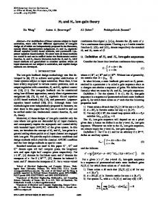
APPENDIX A: SAMPLE INTEGRATION To briefly illustrate the behavior of the above algorithms, let us trace a sample integration. The example is constructed in such a way that major ideas can be presented in a simple way. Example 12. Consider two simple local (object-oriented) schemas given in Fig. 18(a). S:

S 2:

S 1:

human

person

employee student lecturer faculty teaching_assistant

professor

person student employee rules faculty lecturer

professor

teaching_assistant (a)

(b)

Fig. 18. Two simple local schemas and the assertion set defined for them. If the assertion set between them is defined as shown in Fig. 18(b), then an integrated schema as shown in Fig. 18(c) will be generated automatically by executing schema_integration.

589

SCHEMA INTEGRATION

In the following, we will explain the entire process step-by-step. By a computation step, we mean an iteration in schema_integration or an iteration in path_labelling, represented as a pair: the operations executed in this step and the resulting state of Sb or Sd. Note that the state of Sb is changed by executing lines 5-6, 16, 23, 31 and lines 33-35 in schema_integration. schema_integration (S1, person; S2, human): initial step: step1:

source pairs into Sb; Sb state: [(person, human)] pop and check of the pair on the top of Sb: person ∫ human; generation of an integrated class: person; some pairs into Sb; Sb state: [(student, employee), (lecturer, employee)]

step2:

pop and check of the pair on the top of Sb: no assertion between student and employee; all the relevant pairs into Sb; Sb state: [(lecturer, employee), (student, faculty)]

step3:

pop and check of the pair on the top of Sb: lecturer Õ employee; call of path_labelling (lecturer, S2, employee, l): initial step:

node employee into Sd;

step31:

pop of the top element of Sd: employee; check: lecturer Õ employee:

Sd state: [employee]

labelling: employee ; child nodes of employee into Sd; step32:

Sd state: [faculty]

pop of the top elemet of Sd: faculty; check: lecturer Õ faculty: labelling: faculty ; child nodes of faculty

step33:

into Sd: pop of the top element of Sd: professor;

Sd state: [professor]

check: no assertion between lecturer and professor marking professor with *; faculty ¨ professor *; (*since no other nodes appear on the path connecting faculty and professor, no undoing operation will be done.*) generation of is_a (lecturer, faculty); professon has no child nodes and therefore Sd becomes empty;

Sd state: []

labelling: lecturer < , l>; label inheritance for child nodes of lecturer: teaching_assistant < , l>; step4:

some pairs into Sb: Sb state: [(student, faculty), (teaching_assistant, faculty)] pop and check of the pair on the top of Sb: student « faculty; the following rules will be generated: ‹ , , y = x, ‹ , ÿ , ‹ , ÿ .

590

YANGJUN CHEN

some rules for integrated attributes will also be created (see Example 8); step5:

no new pairs into Sb; Sb state: [(teaching_assistant < , l>, faculty)] no checking will be done for the pair on the top of Sb; (*in terms of the relationship of labels and inherited-labels*) no new pairs into Sb and therefore Sb becomes empty;

Sb state: [].

In the above execution, we see that an integrated version for S1(person) and S2(human), a new link connecting faculty and student, and several rules for declaring the semantic relationships among the integrated concepts (derived in terms of local classes: S1(student) and S2(faculty)) are created. Therefore, with our default strategies combined together, schema_integration and path_labelling will produce the integrated schema shown in Fig. 18(c). In addition, the following three features of the algorithms can be observed: 1. In each iteration step of schema_integration, not all relevant pairs are put into Sb. Therefore, the optimization discussed in the previous subsection is implemented. For example, after S1(person) ≡ S2(human) is checked, only (student, employee) and (lecturer, employee) are put into Sb for subsequent checks. (In contrast, in the naive algorithm, pairs such as (student, human), (lecturer, human) and (person, employee) will be put into Sb.) 2. The integration principle for handling is-a paths is correctly realized. For example, only one is-a link between S1(lecturer) ≡ S2(faculty) is created, and all other is-a links such as is_a(IS(lecturer), IS(employee)), is_a(IS(teaching-assistant), IS (employee)) and is_a(IS(teaching-assistant), IS(faculty)) are not considered; they will be redundantly generated if an algorithm like that proposed in [33] is used. 3. By utilizing labels, repetitive checking of “⊆” (or “⊇”) assertions is avoided. For example, pairs such as (teaching_assistant, employee) and (teaching_assistant, faculty) (for which the inclusion assertion is declared) need not be checked. More importantly, the corresponding depth-first searches are also avoided in this way.

APPENDIX B: EVALUATING VIRTUAL RULES In this appendix, we will discuss our strategy for evaluating “virtual” rules to show that our method will not damage the autonomy. Assume that S1 contains two concepts mother and father while S2 contains two other concepts parent and brother. Then, two rules of the following form will be generated in IS1: (1) parent(x, y) ← mother(x, y), (2) parent(x, y) ← father(x, y). If uncle is a concept of S2, then the following rule will be generated in IS2: (3) uncle(x, y) ← parent(x, z), brother(z, y). Given a query of the form ?-uncle(John, y) against IS2, rule (3) will be evaluated. As in a normal deductive database, rules (1) and (2) will be invoked when parent is encountered. But the backward inference process is a bit different. Here, we associate each head predi-

SCHEMA INTEGRATION

591

cate q with a set of schema names S with each one containing q as a concept, and each body predicate p with a set of rules R with each one having p as its head. In this way, the above rules can be rewritten as follows: (1) parent{S2}(x, y) ← mother{ }(x, y), (2) parent{S2}(x, y) ← father{ }(x, y), (3) uncle{S3}(x, y) ← parentr{1, 2}(x, z), brotherr{ }(z, y), (4) mother{S1}(x, y) ←, (5) father{S1}(x, y) ←, (6) brother{S2}(x, y) ←. Note that in the above rules, each basic predicate is represented as a rule with an empty body. Based on the above labeling mechanism, the algorithm for evaluating rules can described as shown below. In the algorithm, q represents a query and Q is a set of rules whose head predicate matches q. Algorithm evaluation(q, Q) begin for each rule of the form: q{S} ← p1{R1}, ..., pn{Rn} ∈ Q do {temp := ∅; for each s ∈ S do (*s repersents a schema name.*) temp := temp ∪ results of evaluating q against s; for each i = 1 to n do tempi := evaluation(pi, Ri); (*recursive call*) temp’ := temp1 ... tempn; result := temp ∪ temp’; } end The above algorithm is just a naive version used to present our idea clearly. As in deductive databases, the constants appearing in the query and the constant propagation can be used to optimize the evaluation process.

Yangjun Chen ( ) received his BS degree in information system engineering from the Technical Institute of Changsha, China, in 1982, and his Diploma and PhD degrees in computer science from the University of Kaiserslautern, Germany, in 1990 and 1995, respectively. From 1995 to 1997, he worked as an assistant professor at the Technical University of Chemnitz-Zwickau, Germany. Dr. Chen is currently a senior engineer at the German National Research Center of Information Technology. His research interests include deductive databases, federated databases, multimedia databases, the constraint satisfaction problem, graph theory and combinatorics. He has published more than 50 works in these areas.