Hugo Grimmettâ , Mathias Buerkiâ¡, Lina Pazâ ,. Pedro Piniesâ , Paul Furgaleâ¡, Ingmar Posnerâ , Paul Newmanâ . â Mobile Robotics Group, University of Oxford, ...
Integrating Metric and Semantic Maps for Vision-Only Automated Parking Hugo Grimmett†, Mathias Buerki‡, Lina Paz†, Pedro Pinies†, Paul Furgale‡, Ingmar Posner†, Paul Newman† †Mobile Robotics Group, University of Oxford, UK {hugo, lina, ppinies, ingmar, pnewman}@robots.ox.ac.uk ‡Autonomous Systems Lab (ASL), ETH Zurich, Switzerland {mathias.buerki, paul.furgale}@mavt.ethz.ch
Abstract— We present a framework for integrating two layers of map which are often required for fully automated operation: metric and semantic. Metric maps are likely to improve with subsequent visitations to the same place, while semantic maps can comprise both permanent and fluctuating features of the environment. However, it is not clear from the state of the art how to update the semantic layer as the metric map evolves. The strengths of our method are threefold: the framework allows for the unsupervised evolution of both maps as the environment is revisited by the robot; it uses vision-only sensors, making it appropriate for production cars; and the human labelling effort is minimised as far as possible while maintaining high fidelity. We evaluate this on two different car parks with a fully automated car, performing repeated automated parking manoeuvres to demonstrate the robustness of the system.
I. Introduction The environments in which our robots operate are often very complex, sharing aspects which are continually evolving along with some much more permanent features. Alongside these varying scales of change, certain tasks required for autonomous operation can be carried out in an unsupervised manner, making them cheap, while others require significant human involvement due to either the difficulty of the task or the need for accuracy guarantees. In this paper we propose a framework which strives for the best of both worlds: we manage the reprocessing of tasks based on how often they require updating, and we streamline tasks which require human involvement while maintaining the accuracies required for safety-critical automated driving. The particular tasks we consider are those of creating metric maps of our robot’s environment, required for path planning, and creating semantic maps which are crucial for the robot’s ability to reason about and interact appropriately with their surroundings. An example of such a map is shown in Fig. 1. We envisage a system by which our metric and semantic maps improve as our robots revisit previously-explored areas, as shown in Fig. 2. In this work we employ vision-only sensors for both mapping and localisation, and so the accuracy of any metric map relies upon the information gathered from the cameras during any particular run. However, the data collected during a revisit can be used to refine the metric map from the previous visit, and that in turn can be used to refine aspects of the semantics.
Fig. 1: The semantic information placed relative to the metric map. Shown are the driving lanes in green, and the parking spaces in blue.
In safety-critical situations such as the operation where automated vehicles and humans coexist, semantic maps are often created (or at least maintained) by hand to ensure their high quality. Here we distinguish between two types of semantic labels: static semantics which represent more permanent features of the environment such as fixed obstacles or points of interaction, and dynamic semantics such as the characteristics of transient objects within an environment. By definition, static semantics are unlikely to change between revisits, and as such represent a significant but necessary cost in terms of human labelling effort, which ideally should not need repeating upon subsequent visits. We use dynamic maps to estimate the likelihood of dynamic obstacles being in any particular location of the robot’s environment, in our case pedestrians, which allows the robot to drive at an appropriate speed. Dynamic semantics can be recomputed at each revisit in an unsupervised manner without requiring further human labelling effort. Once initial semantic and metric maps have been created for a place, subsequent revisits to that place should allow the improvement of those maps without further labelling taking place. More loop closures improve the metric map, and those changes should propagate through to the positions of the semantic labels. We do this by performing the initial labelling in a frame of reference local to the sensor in which the object is visible. This is such that when the metric map is recomputed, the new position of the semantic label is an unmodified local transformation of the newly computed vehicle frame. Fig. 3 demonstrates this principle. As the promise of robots for the general public is increas-
Map$summary$ and$seman-c$ mapping$
static maps and updating the dynamic maps. In Sec. VI we evaluate these systems in a real car park, showing the behaviour following revisits.
Lifelong$Vehicle$ Opera-on$
II. Related Works
Enriched$$ map$data$
Offline$ geometric$ alignment$
Manual$driving$
Updated$ seman-c$and$ localiza-on$ map$
Output$ of$online$ system$ Automated$ driving$
Fig. 2: The cycle of improvement for both metric and semantic maps as a vehicle autonomously revisits a place.
Fs − Ts,v2 !
FO ! −
F v1 ! −
Tv1,g
Tv2,v1
F v2 ! −
Tv3,v2 F v3 ! −
(a) Initial visit
T0v3,v2
Fs ! − F v3 ! −
Ts,v2
F v2 ! −
FO ! − T0v1,G
T0v2,v1
F v1 ! − (b) Revisiting the same place
Fig. 3: While the vehicle positions [v1, v2, v3] may be recomputed between (a) the initial visit and (b) the revisit, the position of the semantic object s relative to v2 remains unchanged. This allows us to update the metric map without having to recreate the semantic labels. FO represents the global origin coordinate frame, and Ta,b represents a 6 d.o.f. transformation from b to a.
ing, parking is a clear early target for widespread automation. The ubiquity of the requirement to park vehicles in car parks motivates the V-Charge project, whose goal is to provide a repeatable, robust, automated valet-parking system which requires neither expensive sensors nor specialised infrastructure in the car parks themselves. The main contributions of this paper are: • The implementation and evaluation of a life-long metric and semantic mapping system on a fully automated car, • The proposal of a lifelong mapping cycle that seamlessly integrates metric map updates with both static and dynamic semantic labels, • An algorithm for automatically generating road network graphs, and • The use of introspective active learning for both parking space detection and pedestrian detection. In Sec. IV we explain the localisation and mapping pipeline. In Sec. V we describe the process of creating the
The field of automated driving has a rich history, gradually making its way into production cars. This push to make robotics relevant for the wider public has led to significant progress in terms of localisation robustness using vision-only systems [1], [2]. Semantic mapping is also a rapidly developing field, but creating reliable maps with vision-only is difficult. Paper [3] fuses laser and camera data to map urban environments. The labelling of parking lots in particular has been approached using overhead images from online photographic repositories (such as Google Maps) [4], but this method makes assumptions about the layouts of parking lots. We assume no particular structure, and label in synthetic overhead maps made by projecting the camera views into simulated ground surfaces, which is useful for mapping underground car parks where satellite imagery is not available. The authors of [5] use a generative model of the geometry of urban scenes to label the lanes and a dynamic map. We overlay this style of map with an extra layer of semantics related to parking and the likely motion of pedestrians. The matter of storing and subsequently making use of semantic labels was tackled during the Urban Challenge, with the road network being hand-labelled and then distributed to the competitors in the RNDF format [6]. The competitors then had to perform automated parking manoeuvres based on these maps [7]. In this work we leverage the adaptability of relative maps. Hybrid topological-metric maps have emerged to be a dominant representation in the field of autonomous driving: examples include sub-mapping [8], to manifold mapping [9], to completely relative representations [10]. We draw from all these influences, but present a robust and well-integrated end-to-end system which generates constantly-improving, rich semantic information and uses it to perform repeated parking manoeuvres with high accuracy. III. The Autonomous Car For the V-Charge project, two VW Golf series vehicles have been modified for drive-by-wire capability, with an integrated camera system, IMU, and computer systems. The test vehicle is equipped with four 180◦ field-of-view fish-eye cameras, one facing each cardinal direction of the car (see Fig. 4). Images are recorded simultaneously at 12.5Hz in gray-scale format with a resolution of 1280 x 960. Subsequent downsampling to half the original size and extraction of BRISK features allows for fast, CPU-based image processing. In addition, wheel odometry running at 50Hz is used as a motion sensor yielding constraints between adjacent image acquisition poses. The intrinsic and extrinsic parameters of the camera system are calibrated using the CamOdoCal library [11].
!
Fig. 4: The configuration of the four 180◦ field-of-view fish-eye cameras used for mapping, localisation, and dynamic object detection.
IV. Metric Mapping In this section, we describe the metric mapping and localisation system which is required for the semantic labelling pipeline, and for autonomous navigation around the car park. For more detail the reader is referred to [12] and [13]. A. Map Representation Let F denote a coordinate frame A, and let further A p → −A denote a point in space expressed with respect to F . In → −A addition to that, let TA,B denote a 6DoF transformation, relating two coordinate frames such that A p = TA,B · B p. We further define F to be an arbitrary, spatially fixed → −O global origin frame. Our map used for localisation can then be thought of as a collection of landmarks Mi p expressed with respect to individual map frames F as well as a set → − Mi of transformations TO,Mi associated with each map frame. Landmarks here refer to 3D points in Euclidean space, associated with a BRISK feature descriptor. As will become clear later, these map frames are fixed in space at all times and lie along the car path of the initial dataset used to form the base-map. The landmarks are originally observed and inferred from the cameras mounted on the vehicle, for which the exact car poses with respect to the global coordinate frame for every captured image is inherently unknown and subject to change as more information becomes available in subsequent mapping sessions. Therefore, the map also contains transformations between vehicle poses and associated mapping frames. During the course of the map refinement, both the location of the landmarks as well as the vehicle poses are updated, whereas the mapping frames stay stationary. B. The Base Map Since the four cameras record images simultaneously, we will refer to an image frame as the collection of all four images recorded at that time. In a first stage, the initial image stream is subsampled such that consecutive image frames are evenly spaced along the car trajectory, separated by a 20cm baseline. A vehicle pose is associated with each of the remaining image frames, forming a posegraph. Subsequently, BRISK features are extracted for each camera image, followed by a loop-closing engine looking for matching images, which then form relative transformation constraints based on a RANSAC estimate of the camera poses of the images involved. Together with the constraints between successive car poses from integrated wheel odometry, a pose-graph relaxation problem is formulated whose solution consists of a geometrically consistent graph of car poses. In the next stage, the BRISK features are tracked along
subsequent images - individually and independently for each camera. The guess of the car poses together with the camera extrinsic and intrinsic calibration allow to infer the landmark positions in the global frame for all feature tracks. Finally, a full bundle adjustment optimisation problem is solved, which involves all landmark observations (reprojection constraints between the inferred 3D landmark position and the observed 2D feature in the images) and all wheel odometry constraints between successive car poses. This yields a refined estimate of the car poses along the pose-graph and all landmarks observed in the base-map. To complete the initial base-map, a mapping frame F is created for each car pose. → − Mi C. Localisation and Multi-Session Mapping With the base-map described in the previous section, the car is able to navigate autonomously within the mapped area. This is achieved by repeatedly estimating the transformation TMi ,v between the car and a nearby map frame. Let Td Mi ,v be a guess of the car’s current pose based on a previous localisation estimate and wheel odometry. We now retrieve the landmarks from the map in the vicinity of our guess and project them into the camera frames, allowing to match them against the extracted image features by taking both the image space and descriptor distance into account when forming the set of 2D-3D associations. From these associations, constraints on the vehicle pose are formed in the context of a non-linear least squares optimisation problem. The vehicle pose is estimated by minimising the reprojection errors based on these associations. This estimate is then used in the proximate iteration as a new starting point. Since between recording the initial dataset for the basemap and a later attempt to localise in it, the environment may change, not all image features will be successfully matched against landmarks from the base-map during localisation. These unmatched features can be used in an offline processing step to track new landmarks which are then added to the base-map, enriching the latter with new information representing the change in the environment. For the reasons mentioned above, we also add the new vehicle poses to the map. Both the new landmarks as well as the new vehicle poses are associated with a nearby map frame. This associations, corresponding to transformations between the new vehicle poses and the fix map frames from the base-map, stem from the localisation estimate based on successfully matching a large enough subset of features in the current image frames to landmarks already present in the map. Consequently, the image frames from the dataset used to localise against the map (subsequently referred to as the “localisation dataset”) contain associations both between landmarks from the base-map as well as the new landmarks and hence allow formulating constraints between the vehicle poses from the base-map and the ones from the localisation dataset. This fact is exploited in a full bundle adjustment step. The resulting map is referred to as a multi-session map now consisting of two datasets. The procedure can naturally be extended to an arbitrary number of datasets. This multi-session mapping allows the map to be refined as more datasets are processed resulting in more accurate map geometry and increased localisation performance. Please note
that the multi-session mapping described in this form does not explicitly deal with landmarks that disappear or shift their position in changing environments over longer time spans. Outdated landmarks remain in the map, but will fail to match against current image observations. This is acceptable as long as a large enough set of valid landmarks can be matched against current images at all times. Also note that, as described above, image features failing to match against the map are tracked over subsequent images and form new landmarks that may account for an outdated landmark that shifted its position or changed its appearance. Techniques to curate maps and filter out outdated or unhelpful are studied in detail in [13]. V. Semantic Mapping In most parking environments there is a wealth of permanent semantic information which can, if correctly leveraged, make a complex manoeuvre such as driving along a lane and parking a much more straightforward task. Typically the creation of such a map involves hand-labelling features such as parking spaces and lanes, but this is an extremely expensive and tedious task for a human. Therefore, we make use of machine learning to reduce the effort on the labeller. In one-shot machine learning, it is necessary to have a large amount of labelled data to train a classifier to detect pedestrians or parking spaces with sufficient accuracy to make it useful, which may not generalise well over car parks. To combat this and also maximise flexibility, we use activelearning algorithms in which a human works in the loop with the machine to answer the most challenging classifications as chosen by the algorithm, thus reducing the labelling quantity for a given desired performance level. In order to further reduce the labelling effort, we make use of introspective active learning algorithms [14]. In the car parks we have encountered during the VCharge project, we have included the following classes in the semantic map: lane structures, parking spaces, pedestrian crossings, and a recommended driving speed for any point in the environment. The recommended driving speed comes from the dynamic map, which brings together permanent aspects of the environment (such as lanes) and dynamic objects such as pedestrians or vehicles. As the automated vehicle drives through the car park, it detects these dynamic objects and incorporates these new observations into the existing map, which better informs the vehicle how to safely navigate the area during future visits. A. Static Map We use active learning on a synthetic overhead image to accurately locate all the parking spaces in the car park. The pedestrian crossings, being so few in number, are labelled by hand. 1) Synthetic overhead image: The synthetic overhead image is made by first rectifying the fisheye images, then using the vehicle pose from the metric map to project the image points onto a virtual ground plane. When projections from multiple images lie on the same pixel in the ground plane, the running mean of the values is used. The overhead images created of the car parks used in the experiments section are shown in Figs. 6 and 11.
2) Classification: From the synthetic overhead image, we train a linear Gaussian process classifier to detect parking spaces. Gaussian process classifiers have been shown to perform well in active learning [15]. Initially the classifier has no training data, and so the user draws rectangles around a few parking spaces. Negative examples are randomly extracted from the image at various scales. Training occurs using the HOG feature [16] representations of these data, and the classifier returns a pre-defined number of hypotheses of where further parking spaces may lie in the image. The hypotheses come from a search over the image at several scales calculated relative to the average size of the user-supplied positive examples, over which non-maximal suppression is applied to increase their positional accuracy. The user then has the option to accept the hypotheses, or mark some of them as positive and negative examples, and retraining the classifier. This cycle can continue until all the parking spaces are detected to a sufficiently high level as set by the user. 3) Relative association: Now that we have the positions of the parking spaces and pedestrian crossings in the synthetic overhead image, for each label we find the fisheye image in which they are visible and most central. We then associate that label with that camera pose, and calculate the transformation between the label and the vehicle pose (Ts,v2 in Fig. 3). This is what allows us to avoid relabelling the static semantic labels whenever the metric map is updated. B. Road Network We have developed an algorithm for automatically generating a road network, whose only requirement is for the vehicle to have been driven through each lane at least once. The algorithm uses only the three-dimensional positions of the vehicle at regular time intervals, and detects both lanes and intersections. The method is presented in Algorithms 1 and 2. In summary, we consider the vehicle positions as nodes in a graph, and connect them to nearby nodes in order to simplify lanes which are driven several times with slight displacement each time (see Fig. 8a). We then repeatedly prune this graph by replacing maximal cliques by their centre point (or rather, an existing node nearest to their centre point, see Fig. 8b) until we have a skeleton graph (see Fig. 8c). The final step involves iteratively exploring the pruned graph to find the distinct lanes and intersection points, as shown in Fig. 8d. C. Dynamic Map We use a probabilistic representation of dynamic obstacles to create a recommended speed map we call the dynamic map. First of all, we project the pixel locations of the static labels into the global frame, obtaining a metrically consistent semantic map. In order to use the semantic map for motion aid we estimate the likelihood of any place in the map x being occupied by a dynamic object, given the prior knowledge of the detected labels at x0 and partial observations of pedestrians z. This posterior distribution is then used to create a recommended speed map for safer future traversals of the car park. Note that the pedestrian detections come from detections in the fisheye images. This
Algorithm 1: Creating and simplifying the adjacency matrix required for Algorithm 2.
1 2 3 4
5 6 7 8 9 10
11 12
13 14 15 16 17 18 19 20
21 22 23 24 25
Data: vehicle poses X ∈ R3 , connecting distance d, number of pruning loops P Result: Symmetric adjacency matrix A // Connect all nodes within a radius d of each other forall the pairs of poses (xi , x j ) ∈ X do if kxi − x j k≤ d then Ai j ← 1 else Ai j ← 0; A ji ← 0 // Symmetric A // Disconnect temporally subsequent nodes within d forall the poses xi ∈ X do n←1 while kxi − xi+n k≤ d // Exit if assertion fails do Ai,i+n ← 0; Ai+n,i ← 0 n←n+1
A ← removeRowsAndCols(R, A) // remove the rows and columns of A which refer to the nodes in R
problem can be represented by a graphical model G(V, E) whose nodes xi ∈ V are the set of discrete map locations. Fig. 5 shows an example of the probabilistic graphical model used in this method. A prior probability p(x0 ) on the nodes is assigned by considering the various types of space encoded in the semantic map (i.e., pedestrian crossings, parking spaces and driving lanes). The maximum a posteriori estimate is calculated by solving: likelihood
(1)
prior
where the prior distribution and pedestrian likelihood are modelled as normal distributions over the map, making the optimisation linear. To account for the effect of a node xi on its neighbours N(i), we impose regularisation by adding linear binary constraints (the second sum in Eq. 2). X X X p(x|x0 ) ∝ k xi − xi0 k22 + k xi − x j k22 (2) i
p(z|x) ∝
i
i
k zi −
xi k22
.
3 4 5 6 7 8 9 10 11
j∈N(i)
(3)
Data: Symmetric adjacency matrix A with M rows and columns Result: Road network R, intersections I ∗ v←∅ // Current node T ←∅ // Termination nodes R←∅ // Road network I ∗ ← {i ∈ {1, . . . , M} for which degreeA (i) > 2} while A nonempty do // Intersection nodes I ← {i ∈ {1, . . . , M} for which degreeA (i) > 2} // Dead-end nodes D ← {i ∈ {1, . . . , M} for which degreeA (i) = 1} if D 6= ∅ then v ← some d ∈ D // Start at a dead-end node T ← I // Terminate at an intersection node else
14
if I 6= ∅ then v ← some i ∈ I T ← I \ {v}
15
else
13
// Prune cliques larger than 2, replacing them by the node nearest to the clique centre for p ← 1 to P do // Produce an ordered list of maximal cliques C ← findMaximalCliques(A) C ← sortDescending(C) R=∅ // The set of nodes marked for removal forall the cliques c ∈ C such that |c|> 2 do xµ ← mean(xc ) xb ← returnNearestNode(xµ , X) N ← returnNeighbours(c, A) // N includes indices i ∈/ c but adjacent to at least one node in c // Skip cliques containing nodes marked for removal if N ∩ R = ∅ then Ab,N ← 1; AN,b ← 1 // Find the dead-end nodes D ← {i ∈ N for which degreeA (i) = 1} // Mark these nodes for removal R ← R ∪ c ∪ D \ {b}
X
1 2
12
// Connect nodes in the order they were driven forall the poses xi ∈ X do Ai,i+1 ← 1; Ai+1,i ← 1
z}|{ � x∗ = arg min − log p(z|x) p(x|x0 ) p(x0 ) , |{z} x
Algorithm 2: Iteratively exploring the adjacency matrix from Algorithm 1 to discover the road network and its intersections.
16 17 18 19 20 21 22 23 24 25 26
// Remaining road network is only one loop v←1 // Start anywhere T ←∅ L←v // Lane O ← returnNeighbours(v, A) // Options while (i ∈/ T ) ∧ (O 6= ∅) do v ← some o ∈ O L ← (L, v) // add v to the vector L O ← returnNeighbours(v, A) \ L // with L as a set R ← R ∪ {L} if L1 ∈ I then L ← L \ L1
// R is a set of vectors // don’t include start node
28
if L|L| ∈ I then L ← L \ L|L|
29
A ← removeRowsAndCols(L, A)
27
// don’t include terminal node
Due to the linear nature of the problem, an exact solution is achieved after a single batch iteration. The final step is to convert the posterior probability of a pedestrian over the car park into a recommended speed profile. We do this by defining minimum and maximum driving speeds, and use the probability to interpolate linearly between the two. A high likelihood of a pedestrian lowers the recommended speed at that location. This produces a map such as those on the right hand side of Fig. 10. VI. Experimental Results In this section we describe the experiments carried out in two different car parks to validate our metric and semantic mapping algorithms, and the manner in which they evolve together. The evaluation is split into two subsections, one for the Stuttgart car park (Sec. VI-A), and the latter for the Zurich car park (Sec. VI-B). A. The Stuttgart Car Park We have run the metric and semantic mapping pipelines described in Sections IV and V using data from a car park in Stuttgart. As a proof of concept, we drove the car manually around the car park several times. This car park contains 164 parking spaces. The lighting conditions during the data collection were consistent in the middle of the car park,
Fig. 6: The synthetic overhead image from the Stuttgart car park. The car park is larger and the image much cleaner than that of the Zurich car park, and so is better suited to active learning.
Fig. 5: The graphical model used to represent the probability distribution of pedestrians. White nodes x correspond to the set of discrete map locations. Blue nodes x0 represent values after applying the initial prior probability on a subset of nodes according to their classification as parking spots, pedestrian crossings, lanes, or other. Green nodes z correspond to the observations of dynamic objects in a particular map location. Note that a dynamic object could be observed multiple times (za1 , za2 ) at the same location a, thus a node xa would updated with several observations.
becoming brighter closer to the long edges (which receive more natural light). The synthetic overhead image does not have too many undesirable artefacts (see Fig. 6). We then use active learning to detect the parking spots in the synthetic overhead image. In total, the user only had to manually label 14 parking spaces over 6 rounds of active learning to achieve a precision of over 0.93 (see Fig. 7), which substantially reduces the human effort in such a labelling task. In addition, if we were to map further floors of this car park, the classifier learned from this floor could be applied to those to make the process very easy for the labeller. Note that the number of times the user accepts or rejects the hypotheses returned by the classifier at each round of training is not shown. This feedback is very quick and is a negligible contributor to the labelling effort. A further note is that the only negative examples in the training data were rejected hypotheses from the classifier, thus at epoch 1 there is only one negative: the vector 0. In Fig. 8 we show some of the intermediary steps and the final result of the road network generation algorithm on the Stuttgart car park. In a totally unsupervised manner (aside from choosing the parameters r and p for Algorithm 1) the entire road structure is extracted from the poses. This road structure together with the parking spots could now be used for autonomous driving. We also detect pedestrians and process the dynamic map for this car park, but this is not shown. For a demonstration of this, see Sec. VI-B. B. The Zurich Car Park For the evaluation of the improvement cycle and automated parking we use an underground car park in Zurich.
Fig. 7: The precision of the parking space detections (blue) across active learning loops. The cumulative number of hand-drawn labels is shown as the dashed green line. Note that at each loop, the user specifies some of the classifier hypotheses as correct and incorrect, and these are not shown as they are much quicker to input than drawing new labels from scratch.
Fig. 9: The car park in Zurich. Note the difficult lighting conditions, resulting in glare off the ground.
There are 80 parking spaces which vary in size depending on their position relative to the edges and corners. The parking spaces are delineated by yellow markers as shown in Fig. 9. The car park is not planar; there is a drain running along the centre, and the ground is hinged at this point all the way to the edges. Some of the yellow lines on the floor are omitted in favour of yellow columns, as pictured. There are two pedestrian crossings, one is shown in the figure as yellow hatching on the right. The data are organised as follows: the car was driven twice around the car park as an initial visit, and then there were six subsequent ‘revisit’ loops. During each revisit loop, pedestrians walk between the pedestrian crossings; in revisit loops 1 to 3, they walk along the right-hand pedestrian crossing, and then in loops 4 to 6 they walk along the lefthand pedestrian crossings, as shown in the left hand side of
(a) The fully connected graph (b) The graph after one pruning (c) The finished graph at the end (d) The lanes as calculated by (Algorithm 1, lines 1 to 12). loop (Alg. 1, lines 13 to 25). of Alg. 1. Alg. 2. Fig. 8: The process of calculating the road network using the method from Sec. V-B applied to the Stuttgart car park.
(a) Initial drive. Fig. 11: The synthetic overhead image of the Zurich car park.
(b) The maps from data up to and including the 3rd revisit.
(a) Initial visit
(c) The maps from data up to and including the 6th revisit. Fig. 10: On the left, the red dots represent projections of the detected pedestrians into the static map. On the right, the evolution of the dynamic map as more pedestrians are detected. In the dynamic map, blue represents lower danger (higher speed) and yellow represents more danger (higher speed). The top dynamic map is calculated using only the prior over pedestrians given the static map.
(b) First revisit
Fig. 10. We then use these loops to emulate the process in Fig. 2: the first map (comprising both metric and semantic components) is created using the initial run, then as we go around the evolution cycle, the next map comprises the initial loop plus the 1st revisit. The third map comprises the initial run, the 1st and 2nd revisits, and so on. In total we have seven maps, each more informed than the previous one. Because we want to minimise the human labelling effort, we only label the parking spaces and pedestrian crossings once, in the base map. The synthetic overhead image used for creating those labels is shown in Fig. 11. However, because the labels are associated with the vehicle positions from which they were visible in the images, the changes in the metric map shifts the global positions of those semantic labels as the maps evolve. This evolution process is shown
Fig. 12: The evolution of the semantic map through the original drive, and the first revisit. The parking spaces are the orange rectangles, lanes are in blue and the intersections are purple circles. Notice that the top and middle rows of parking spaces shift visibly from (a) to (b) as the changes in the metric map propagate through to the positions of the semantic labels.
in Fig. 12. Note that the overhead image for the Zurich car park is much more distorted and blurry than the one for the Stuttgart car park. This reduces the effectiveness of active learning, and generally the human will have to do more manual labelling if this is the case. Secondly, the positions of the semantic labels do visibly change between the first and second maps in Fig. 12. Next we use the first four maps to test the repeatability of the autonomous parking system. We performed the following actions: 1) The car is driven to a point 20m away from the desired
continuously improving as an autonomous vehicle revisits previously explored locations. We have shown that parking accuracy using these maps is consistently good as these revisits and map refinements take place. The whole framework is streamlined in terms of reducing the human supervision effort, while maintaining the high degree of accuracy required for autonomous operation. We have demonstrated the stability of the system on two car parks as part of the VCharge project. VIII. Acknowledgements Fig. 13: The positions of the five autonomous parking manoeuvres of the vehicle in map for maps 0 to 3. Map 0 comprises the initial drive, then map 1 includes both the initial drive and the 1st revisit, then map 2 includes those for map 1 plus the 2nd revisit, and so on. The displacement between the parking centres and the position of the parking spot (at the origin) is due to the difference between the vehicle centre and the centre of the parking spot.
parking location, then 2) The car localises itself in the metric map and uses the semantic map to drive autonomously along the lane and park in the parking space. 3) Next, the car is manually driven out of the parking space to the same starting location 20m away, and the process is repeated for a total of five times per map. Calculating the ground truth of localisation systems for mobile platforms is an open problem, so we have done this by estimating the position of the vehicle relative to a chequerboard at a fixed position in the car park which is visible in the camera images. The parking positions are shown in Fig. 13. This shows that despite the fact that the metric maps are recalculated in an unsupervised manner and the positions of the semantic labels shift acoordingly, the parking accuracy is very consistent, with a significant cluster of points within 0.13m and the few outliers never varying by more than 0.3m. We attribute these outliers to errors in the odometry, and the fact that the parking planner plotted a bad course for the vehicle during one of the parking manoeuvres during the first revisit. Evolution of the speed map: During the initial drive there are no pedestrians in the car park, but during each revisit there are pedestrians walking along the pedestrian crossings. Using the same active learning framework explained in Sec. V-A.2 applied to the raw camera images, we detect these pedestrians and then using the method detailed in Sec. V-C we update the dynamic map. This dynamic map represents the recommended driving speed for subsequent visits to the car park. In Fig. 10 we show the positions of the pedestrians as red points on the left, and the evolution of the dynamic map on the right. It is also convenient that as we see more pedestrians, the classifier becomes increasingly good at detecting them, thus reducing the human labelling effort as time goes on. VII. Conclusions We have presented a functioning end-to-end system which provides a solution to the question of how metric and semantic maps should be fused together. This approach has been framed within with principle that maps should be
This work is funded under the European Community’s Seventh Framework Programme (FP7/2007-2013) under Grant Agreement Number 269916 and by the UK EPSRC Grant Number EP/J012017/1. References [1] P. Furgale, U. Schwesinger, M. Rufli, W. Derendarz, H. Grimmett, P. Muhlfellner, S. Wonneberger, J. Timpner, S. Rottmann, B. Li, et al., “Toward automated driving in cities using close-to-market sensors: An overview of the V-Charge Project,” in IEEE Intell. Vehicles Symposium (IV), 2013. [2] U. Franke, D. Pfeiffer, C. Rabe, C. Knoeppel, M. Enzweiler, F. Stein, and R. G. Herrtwich, “Making Bertha See,” IEEE ICCV Workshop Computer Vision for Autonomous Vehicles, 2013. [3] B. Douillard, D. Fox, F. Ramos, and H. Durrant-Whyte, “Classification and Semantic Mapping of Urban Environments,” The Intern. Journal of Robotics Research (IJRR), 2011. [4] Y.-W. Seo and C. Urmson, “A Hierarchical Image Analysis for Extracting Parking Lot Structures from Aerial Images,” Tech. Rep., 2009. [5] A. Geiger, M. Lauer, and R. Urtasun, “A Generative Model for 3D Urban Scene Understanding from Movable Platforms,” in IEEE Conf. on Computer Vision and Pattern Recognition (CVPR), 2011. [6] D. U. Challenge, “Route Network Definition File (RNDF) and Mission Data File (MDF) formats,” Tech. Rep., Defense Advanced Research Projects Agency, Tech. Rep., 2007. [7] M. Montemerlo, J. Becker, S. Bhat, H. Dahlkamp, D. Dolgov, S. Ettinger, D. Haehnel, T. Hilden, G. Hoffmann, B. Huhnke, et al., “Junior: The Stanford Entry in the Urban Challenge,” Journal of Field Robotics, 2008. [8] J. Guivant and E. Nebot, “Improving Computational and Memory Requirements of Simultaneous Localization and Map Building Algorithms,” in IEEE Intern. Conf. on Robotics and Automation (ICRA), 2002. [9] A. Howard, G. S. Sukhatme, and M. J. Matari´c, “Multi-Robot Mapping using Manifold Representations,” IEEE - Special Issue on Multi-robot Systems, 2006. [10] G. Sibley, C. Mei, I. Reid, and P. Newman, “Planes, Trains and Automobiles Autonomy for the Modern Robot,” in IEEE Intern. Conf. on Robotics and Automation (ICRA), 2010. [11] L. Heng, B. Li, and M. Pollefeys, “Camodocal: Automatic Intrinsic and Extrinsic Calibration of a Rig with Multiple Generic Cameras and Odometry,” in IEEE/RSJ Intern. Conf. on Intelligent Robots and Systems (IROS), 2013. [12] P. Muehlfellner, P. T. Furgale, W. Derendarz, and R. Philippsen, “Evaluation of Fisheye-Camera Based Visual Multi-Session Localization in a Real-World Scenario,” in IEEE Intell. Vehicles Symposium (IV), 2013. [13] P. M¨uhlfellner, M. B¨urki, M. Bosse, W. Derendarz, R. Philippsen, and P. Furgale, “Summary Maps for Lifelong Visual Localization,” 2014, manuscript submitted for publication. [14] H. Grimmett, R. Paul, R. Triebel, and I. Posner, “Knowing When We Dont Know: Introspective Classification for Mission-Critical Decision Making,” in IEEE Intern. Conf. on Robotics and Automation (ICRA), 2013. [15] R. Triebel, H. Grimmett, R. Paul, and I. Posner, “Driven Learning for Driving: How Introspection Improves Semantic Mapping,” in Intern. Symposium on Robotics Research (ISRR), Singapore, 2013. [16] N. Dalal and B. Triggs, “Histograms of Oriented Gradients for Human Detection,” in IEEE Conf. on Computer Vision and Pattern Recognition (CVPR), 2005.