Integrating multiple data sources for assessing ... - Wiley Online Library

DOI: 10.1111/ddi.12739

BIODIVERSITY RESEARCH

Integrating multiple data sources for assessing blue whale abundance and distribution in Chilean Northern Patagonia Luis Bedriñana-Romano1,2

 | Rodrigo Hucke-Gaete1,2 | 

Francisco Alejandro Viddi1,2 | Juan Morales3 | Rob Williams4 | Erin Ashe4 |  José Garcés-Vargas1,5 | Juan Pablo Torres-Florez2,6 | Jorge Ruiz1,2 1 Facultad de Ciencias, Instituto de Ciencias Marinas y Limnológicas, Universidad Austral de Chile, Valdivia, Chile 2

NGO Centro Ballena Azul, Valdivia, Chile

3

LaboratorioEcotono, INIBIOMACONICET, Universidad Nacional del Comahue, Bariloche, Argentina 4

Oceans Initiative, Seattle, WA, USA

5

Abstract Aim: Species distribution models are useful tools for depicting important habitat, assessing abundance and orienting conservation efforts. For small populations in poorly studied ecosystems, available data are often scarce and patchy. To overcome this limitation, we aim to evaluate the use of different data types within a hierarchical Bayesian framework with the goal of modelling the abundance and distribution of a

Centro FONDAP de Investigación en Dinámica de Ecosistemas Marinos de Altas Latitudes (IDEAL), Valdivia, Chile

small and highly migratory population of blue whale (BW, Balaenoptera musculus)

6

Departamento de Genetica e Evolução, Universidade Federal de São Carlos, São Carlos, SP, Brazil

Location: CNP, Eastern South Pacific (ESP).

Correspondence Luis Bedriñana-Romano, Facultad de Ciencias, Instituto de Ciencias Marinas y Limnológicas, Universidad Austral de Chile, Valdivia, Chile. Email: [email protected]

line-­transect data (2009, 2012 and 2014) with a logistic regression for modelling

Funding information Fondo Nacional de Desarrollo Regional, Gobierno Regional de Los Lagos, Grant/ Award Number: BIP N°30040215-0 ID1857-17LP07; Whitley Fund for Nature; Kilverstone Wildlife Charitable Trust; World Wildlife Fund (WWF) Germany Editor: Clare Embling

summering in Chilean Northern Patagonian (CNP). Methods: We constructed a Bayesian hierarchical species distribution Model (HSDM), combining a binomial N-­mixture model used to model BW groups counts in presence-­availability data (2009–2016), allowing both models to share covariate parameters for borrowing strength in estimations. Results: Distance to areas of high chlorophyll-­a concentration during spring before summering season (AHCC-­s) was the most important and consistent explanatory variable for assessing BW abundance and distribution in CNP. Incorporating accessorial presence-­only data reduced uncertainty in parameters estimation when comparing with a model using only line-­transect data, although other covariates of secondary importance failed to be retained in this model. Main conclusions: Our results remark the capability of HSDM for integrating different data types providing a potential powerful tool when data are limited and heterogeneous. Results indicate that AHCC-­s, and possibly thermal fronts, could modulate BW abundance and distribution patterns in CNP. Preliminary model-­based delimitations of possible priority conservation areas for BW in CNP overlap with highly used vessel navigation routes and areas destined to aquaculture. KEYWORDS

abundance assessment, blue whale, Chilean Patagonia, habitat selection, hierarchical Bayesian models, marine conservation, species distribution models

Diversity and Distributions. 2018;1–14.

wileyonlinelibrary.com/journal/ddi   © 2018 John Wiley & Sons Ltd |  1

|

BEDRIÑANA-­ROMANO et al.

2      

1 |  I NTRO D U C TI O N

BW prey, are in turn associated with the upwelling process itself (e.g., distance to shelf edge, sea surface temperature (SST) and

Located in the Eastern South Pacific (ESP), Chilean Northern

sea surface height: Croll et al., 2005; Fiedler et al., 1998; Gill et al.,

Patagonia (CNP) represents a region of both elevated primary and

2011; Redfern et al., 2017; Visser, Hartman, Pierce, Valavanis, &

subsequent secondary productivity, which are mainly mediated by

Huisman, 2011). However, CNP is a transitional zone between

the interplay of a large input of low salinity micronutrient-­loaded

areas of seasonal upwelling dominance and areas of perma-

superficial fresh water, high salinity macronutrient-­ loaded oce-

nent downwelling dominance (south of 45° S), thus presenting a

anic deeper water and drastic seasonal changes in light regimes

large synoptic variability even during spring/summer “upwelling-­

(González et al., 2011; Iriarte, González, & Nahuelhual, 2010; Torres

favourable season” (Strub, Mesias, Montecino, Rutllant, & Salinas,

et al., 2011). These complex oceanographic processes sustain a high

1998). In this scenario, most covariates associated with the occur-

but poorly studied marine biodiversity, including the most important

rence of upwelling waters are not expected to be directly transfer-

summering and nursing area for the endangered blue whale (BW,

able to CNP as proxies for krill availability (Redfern et al., 2017).

Balaenoptera musculus) in the ESP (Hucke-­Gaete, Osman, Moreno,

Based in BW (and other large whales) ecology and CNP oceano-

Findlay, & Ljungblad, 2004; Hucke-­Gaete, Ruiz, & Alvarez, 2010;

graphic characteristics, two main environmental factors could be

Reilly et al., 2008). It also hosts one of the largest aquaculture indus-

inspected when assessing BW distribution and abundance. First,

tries in the world (Buschmann et al., 2006; Niklitschek, Soto, Lafon,

because krill abundance in coastal areas is typically positively

Molinet, & Toledo, 2013).

correlated with high phytoplankton concentrations (Feinberg &

Balaenoptera musculus are a local priority for conservation

Peterson, 2003; Riquelme-­B ugueno et al., 2013; Tanasichuk 1998),

and marine spatial planning initiatives (Hucke-­Gaete et al., 2010;

chlorophyll-­a (chl-­a) concentration is commonly used as a useful

Outeiro et al., 2015) due to potential threats, including ship strikes,

proxy for krill availability (Buchan & Quiñones, 2016; Branch et al.,

fishery and aquaculture net entanglement, poorly regulated whale

2007; CPPS 2014; Croll et al., 2005; Zerbini et al., 2016). Within

watching activities and noise (Colpaert, Briones, Chiang, & Sayigh,

CNP, spatio-­temporal patterns in chl-­a distribution have revealed

2016; Hoyt & Iñíguez, 2008; Hucke-­Gaete et al., 2010, 2013; Van

sharp differences among distinct microbasins (González et al.,

Waerebeek et al., 2007; Viddi, Harcourt, & Hucke-­ Gaete, 2015).

2010, 2011; Montero et al., 2011; Tello & Rodriguez-­B enito, 2009),

Thereby, reliable spatially explicit density maps for spatial planning

which should affect BW distribution. Second, thermal fronts (TF)

and risk assessment are needed (Pennino et al., 2017; Redfern et al.,

are mesoscale phenomena that not only influence primary produc-

2013; Williams et al., 2014). Additionally, a new US trade rule re-

tivity but might also elicit a herding effect on small fish and zoo-

quires countries, including Chile, to demonstrate that their fishery

plankton biomass such as krill (Acha, Mianzan, Guerrero, Favero, &

and aquaculture activities are comparable in effectiveness to the US

Bava, 2004; Doniol-­Valcroze et al., 2007; Littaye, Gannier, Laran, &

Marine Mammal Protection Act or risk losing the ability to export

Wilson, 2004; Lutjeharms, Walters, & Allanson, 1985). These phe-

seafood products to the lucrative US market (Williams, Burgess,

nomena could be particularly important in areas with a significant

Ashe, Gaines, & Reeves, 2016). These national and international ef-

freshwater discharge (Sharples & Simpson, 1993) such as CNP. For

forts create a pressing need for information on BW abundance and

BW, the concentrating effect of TF could be crucial because of it,

distribution in the region.

energetically costly feeding behaviour (Acevedo-­G utierrez et al.,

During 2009, private and public agencies joined efforts to

2002; Potvin et al., 2009), that to be cost-­effective, requires krill

generate the first abundance estimate for BW in CNP covering

not only to be abundant, but also highly concentrated (Goldbogen

most of its coastal waters, as part of a broader initiative setting

et al., 2011, 2015).

a baseline for the implementation of a multiple-­u se marine pro-

To test the hypothesis that areas of high chl-­a concentration and/

tected area (Hucke-­G aete et al., 2010). After 1,278 km of dedi-

or areas of recurrent TF trigger higher BW abundance and therefore

cated marine survey, only 33 BW groups were recorded on-­effort

modulates its distribution in CNP, we constructed a hierarchical spe-

yielding an abundance estimate of 222 (115–430) for an area of

cies distribution model (HSDM) integrating classical distance sam-

34,899 km 2 , using classic design-­b ased distance sampling analy-

pling methods, a collection of independent BW sightings database

sis (Hucke-­G aete et al., 2010). To date, no similar survey has ever

(presence-­ only), and oceanographic data obtained from satellite,

covered the extension of 2009 survey in CNP, yet over the years,

over a period of 8 years (2009–2016).

heterogeneous data on BW distribution (i.e., smaller line-­t ransect surveys and opportunistic sightings database) have become available. This poses a major challenge to address BW abundance and distribution patterns in CNP and pleas for integrating these dissimilar data in one comprehensive species distribution model

2 | M E TH O DS 2.1 | Line-­transect surveys

(SDM, Elith & Leathwick, 2009), provided a biological hypothesis

Line-­t ransect surveys were carried out off CNP (41°00′S–45°30′S)

exists.

during austral summer of 2009 and early autumns of 2012 and

In other parts of its range, BW distribution has been tied to

2014, covering distinct but overlapping areas and never exceed-

upwelling-­ modified highly productive waters. Krill, the primary

ing ca. 25 km from the nearest coast (Figure 1). Field protocols

|

      3

BEDRIÑANA-­ROMANO et al.

Gulf and Reloncavi Sound during summer/autumn of 2004–2016 (Figure 1). These surveys were undertaken mostly on board a 7.6-­m semi-­rigid hull inflatable vessel. Additional surveys from exploratory flights or cruise expeditions that were not specifically aimed for marine mammal research were also available, covering other areas of CNP. During all these surveys, observers recorded the groups’ geographical position using a handheld GPS, time of sighting and group size. Only data from 2009 to 2016 were used in subsequent modelling because before 2009, data were restricted to CGMC. This yielded a total of 180 BW groups GPS locations; however, as these data are likely to be highly spatially and temporally auto-­correlated, we used a raster with grid cells of 8 km per side from the study area as sampling units and assigned a value of 1 on each grid cell that presented at least one BW sighting on it for each year. Grid cells with BW sightings in more than 1 year were not considered duplicates as their associated covariates were different. This resulted in a database of 81 blue whale presences for analysis.

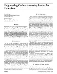
2.3 | Satellite oceanographic and topographic covariates Chl-­a concentration data were extracted from satellite level 3 images from the Moderate Resolution Imaging Spectroradiometer (MODIS) sensor onboard the Aqua satellite (Data set ID: erdMH1chlamday), corresponding to monthly averages in a grid size of 4.64 km. Based on these images, four different covariates were constructed, (1) F I G U R E   1   Map of Chilean Northern Patagonia depicting relevant geographical landmarks. The light-­blue polygon represents the study area comprising waters within 25 km from the coast. Squares represent 8 × 8 km segments of transects undertaken during 2009 (open black contoured squares), 2012 (roughed brown filled squares) and 2014 (filled blue squares). Black dots indicate grid-­cell centroids where presence-­only data were available

spring average chl-­a concentration: generated by a composite of satellite images from September, October and November (austral spring) from the year before (2008–2015) each selected field season (2009–2016); (2) summer average chl-­a concentration: the same as the later but using images from January, February and March of each selected field season (2009–2016); (3) distance to areas of high chlorophyll-­a concentration during spring (AHCC-­s): consisted in distance to polygons enclosing areas with an average chl-­a concentra-

followed standard line-­t ransect survey methods (Buckland et al.,

tion equal or higher than 5 mg/m (Montero et al., 2011) during spring

2001) with some specific modifications for small-­ b oat surveys

months; and (4) AHCC-­su: the same as the later but using summer

(Dawson, Wade, Slooten, & Barlow, 2008; Williams et al., 2017).

months.

A 17-­m motor vessel was used for most surveys, except for the

Daily averages level 4 SST satellite images were obtained from

exposed western coast of Chiloe Island during 2009 where a 17-­m

Multi-­ Scale Ultra-­ High Resolution (MUR) SST Analysis database

sailboat was used. The observer team comprised three persons,

(Data set ID: jplMURSST41). MUR-­SST maps merge data from dif-

plus a fourth person operating the computer to enter data. An

ferent satellites, combined with in situ measurements, using the

angle board mounted on the deck was used to measure radial angle

Multi-­Resolution Variational Analysis statistical interpolation (Chin,

to the group of animals, and visual distance estimate to the animals

Milliff, & Large, 1998), in a grid size of 0.01° (ca. 1 km2). From MUR-­

was estimated at first sighting. To calibrate visual distance estima-

SST maps, thermal fronts (TF) were identified using a single-­image-­

tion, radial distance estimates from observer-­specific estimations

edge-­detection (SIED) algorithm with a threshold detection of 0.5°C

were corrected (Williams, Leaper, Zerbini, & Hammond, 2007)

(Cayula & Cornillon 1992; Cayula & Cornillon 1995). SIED tools were

using known distances from landmarks (i.e., islands, lighthouses,

available in ArcMap 10.1 through the Marine Geospatial Ecology

salmon farms and other vessels) derived from the vessels′ radar.

Tools (Roberts, Best, Dunn, Treml, & Halpin, 2010). Areas of thermal front recurrence (ATFR) were constructed using SIED on daily im-

2.2 | Presence-­only data

ages ranging from 1 January to 30 April for each year skipping every third day for time-­saving purposes during data analysis. A composite

Focal-­ group marine surveys were undertaken in the Corcovado

of this set was used to account for the times each grid cell within the

Gulf and Mouth of the Moraleda Channel (hereafter CGMC), Ancud

study area was catalogued as holding a TF during the 4 months span

|

BEDRIÑANA-­ROMANO et al.

4      

of every year. These new rasters presented grid cell values in a range

Instead of assuming the observed number of BW groups ni in

of 0–16 TF detections within the 4 months’ time span. Percentiles

each track as the true local group abundance (Ni), a second part

for all rasters were very similar across years showing that 90% of the

relates ni to Ni as a binomial outcome with probability of success

grid cells for the entire study area presented three or less TF detec-

determined by detection probability pi , thus making Ni a latent

tions. Therefore, we selected a threshold value of 4 for construct-

variable.

ing polygons yielding ATFR, which only represent areas where the

{ } Pr ni |Ni ,pi =

strongest and most conspicuous TF occur. Distance to these ATFR polygons was used as a covariate in the subsequent models. Summer SST was extracted from level 3 monthly composites from the Aqua MODIS satellite database in a grid size of 4 km (Data set ID: erdMH1sstdmday). Data from January to March of every year (2009–2016) were averaged and this composite was used for data extraction. Raw data for depth were obtained from the Chilean Navy (Servicio Hidrográfico y Oceanográfico de la Armada), from which a triangular irregular network (TIN) model was created using 3D Analyst in ArcGIS and the resultant raster was used to extract depth values. Distance to the coast (DTC) was extracted in QGIS (QGIS Development Team, 2009) and was also used as a covariate.

(

Ni ni

)

( )N −n pi ni 1 − pi i i

Assuming a truncation distance of 4 km, the probability of detection pi was derived from un-­binned perpendicular distances yd from each

d

detection, using a half-­normal distribution with a sin-

gle parameter Σ. Even when we did not use covariates for modelling Σ, i subscript still applies to pi to account for differences in Habitati (Chelgren et al., 2011). Error in distance estimation was assessed by regressing estimated training distances to a series of landmarks by observers against trues distances provided by the vessel′s radar. The slope of this linear regression (Figure S1.1) was used to divide angular distances to BW groups previously to multiplying by the sine of the angle in perpendicular distance estimation (Hammond et al., 2002). Maps of whale densities predictions and associated uncertain-

2.4 | Modelling approach We divided on-­effort tracks from line-­transect surveys into contiguous equal-­sized sampling segments (Hedley & Buckland, 2004; Williams, Hedley, & Hammond, 2006) of 8 km per side (64 km2). For each one of these sampling segments (hereafter tracks), a response variable, BW group counts and environmental covariates were extracted assuming the centroid of each track as the spatial point from which the covariates were extracted. Before analyses, all variables were standardized and correlations were assessed through Pearson correlation analysis. Based on the binomial N-­mixture model from Chelgren et al. (2011), true BW group abundance Ni for each track i was modelled by a Poisson distribution, which we modified to be modelled through a zero-­inflated version

ties from 2009 to 2016 were calculated using rasters of the entire study area with a grid-­cell size of 8 km per side. Model′s estimated parameters were used to predict the number of whales in each grid cell, based on their standardized covariates values, estimated mean group size and estimated intercept parameter for the corresponding year if line-­transect data were available or drawing an intercept value from the normal distribution of intercepts if not. As the bulk of the data was gathered in 2009, we provide an overall abundance estimate only for this year, which was equal to the sum of all grid-­cell values in that year. As a measure of goodness-­of-­fit, we conducted a posterior predictive check (PPCheck, Gelman, Meng, & Stern, 1996) based on chi-­ squared tests, which allowed us to calculate the ratio between the sum of discrepancy measures in observed and simulated data, the c-­hat parameter, and a Bayesian p-­value, which is the probability to

} ∑ λi Ni e−λi Pr Ni > 0 = ψ Ni !

obtain a test statistic that is at least as extreme as the observed test

where ψ is the probability of a non-­zero true abundance and λi is

good fit, Kery & Royle, 2015). All previously described steps were

the usual Poisson parameter, which depends on the exponential of a

undertaken from within the HSDM as a one-­stage approach (Miller,

linear function of covariates

Burt, Rexstad, & Thomas, 2013).

{

λi = Habitati ∗ e(β0y + βXi ) Habitat i is an offset term accounting for effective area sampled at each transect (subtracting land cover when required), β 0,y are intercepts which are calculated for each year y, β is a vector of parameters coefficients and Xi is the corresponding design matrix. Intercepts (β 0,y) were assumed to come from a normal distribution, for which we estimated its respective mean and variance hyperparameters. If required, model selection was performed through a “model identity” variable with each category representing a unique set of covariates, allowing to draw a posterior probability for each one from within the HSDM (Kruschke, 2014; Royle, Chandler, Sollmann, & Gardner, 2013).

statistic computed from the actual data (should be around 0.5 for a

Presence-­availability set-­ups are often modelled through a logistic regression that uses values of “one” for the recorded presence of the species and “zeros” for a sample of randomly selected points within the study area, termed pseudo-­absences or availability data. Aarts, Fieberg, and Matthiopoulos (2012) have shown that count, presence–absence and logistic regression models are all approximations of the inhomogeneous Poisson point process, for which the linear predictor function is proportional to the expected density of observations. Based on this, an alternative model (model 2) incorporated a logistic regression model for the presence-­only data sharing covariate parameters with those of the main count model to borrow strength in estimations. To assess how the subjective process of

|

      5

BEDRIÑANA-­ROMANO et al.

availability data selection (Beyer et al., 2010) influenced the new co-

on these results, we used AHCC-­s in all further models yielding

variate parameters, we constructed five alternative model variants

five variables to be tested in both models, AHCC-­s , ATFR, SST,

using different number of availability points and changing the geo-

DTC and depth.

graphical areas where these points were extracted from (Figure 2).

Model 1 retained AHCC-­s, ATFR, SST and DTC. An interaction

As sample size was small, we also repeatedly ran the model leaving

parameter between the two most important covariates (AHCC-­s and

one data value out every time to check how the parameters poste-

ATFR) was evaluated but not retained by the model. Only AHCC-­s

rior distribution fluctuates.

was retained by model 2 regardless of modifications on availability

All models were fit in R (R Development Core Team 2015) and

data selection (Table S1.1). AHCC-­s was the only covariate retained

JAGS (Plummer, 2003) for Markov Chain Monte Carlo estimation

in all models, experiencing a reduction in the CI and SD of parameters

methods. Vague priors were used for all parameters. Three chains

involved in calculating λ, when incorporating accessory presence-­

were run in parallel through 100,000 iterations each. The first

only data (Table 1). For 2009, the year with more data available,

20,000 samples were discarded as burn-­in, and one of every two

model 2 predicted larger total abundance (442, CI: 236–744) when

remaining samples was retained, for a total of 120,000 samples to

comparing to model 1 (373, CI: 191–652). PPCheck results indicated

form the posterior distribution of model parameter estimates. See

that c-­hat and Bayesian p-­value presented values very near 1 and .5,

Appendix S1 for more details about methods and results.

respectively, indicating a good fit of the model to the data (Table 1

The 2009 abundance estimate and associated credible interval

and Figure S1.3). Removing one sampling unit from analysis at a time

were used to estimate a precautionary minimum abundance esti-

did not produced large differences in parameters posterior distribu-

mate (N min) to estimate a sustainable annual allowable harm limit

tion (Figure S1.4).

from all anthropogenic sources of mortality, namely the “poten-

Plots of predicted density using both models showed a large

tial biological removal” (“PBR,” Wade, 1998). Under US legislation,

variation in BW distribution among years (Figures 3 and 4). Although

PBR is defined as the product of a minimum estimate of abun-

some areas such as Ancud Gulf and the Western Coast of Chiloe

dance (N min) times one half of the maximum net productivity of a

showed some consistency in concentrating higher BW densities,

stock (0.5 Rmax ) times a recovery factor (Fr) between 0.1 and 1.0

overall predictions uncertainty for those years where line-­transect

(Wade, 1998). Guidelines for assessing marine mammal stocks are

data were not available was large (Figure 3). To get a more straight-

well established in the United States, and we follow convention

forward comparison between models, we reran both models using

sing the 80th percentile of the distribution as our value for N min

only AHCC-­s as covariate and focused only on those years where

and a 4% default value for Rmax (Wade, 1998). The recovery fac-

line-­ transect data were available to show how predictions un-

tor is a precautionary adjustment term governing the desired rate

certainty was reduced when incorporating presence-­ only data

of recovery. We follow recommendations for recovery factors for

(Figures 2 and 4).

endangered marine mammals and use a value of 0.1 for Fr (Taylor, Michael, Heyning, & Barlow, 2003).

The point estimate of abundance in 2009 was 373 (model 1). Using 274 as the 20th percentile of the posterior distribution of N, we estimate a potential biological removal of 0.548, or one human-­

3 | R E S U LT S On-­effort tracks comprised 106 sampling units for 2009 (848 km), 35 for 2012 (272 km) and 47 for 2012 (368 km) (Figure 1). A total of 44 BW sightings were observed while on effort during all three

caused death or serious injury every 1.8 years.

4 | D I S CU S S I O N 4.1 | Modelling approach

line-­transect surveys (2009 = 34, 2012 = 2, and 2014 = 8). Three

Literature provides several options to model abundance and distri-

sightings from 2009 were excluded after truncation of perpendicu-

bution from non-­systematic line-­transect effort and sightings data

lar distance data (4 km) yielding 41 sightings for analysis, including

(Hedley, Buckland, & Borchers, 1999; Redfern et al., 2006; Miller

fitting the half-­normal detection function (Figure S1.2). Group size

et al., 2013; and original references cited therein). Pooling all available

ranged between 1 and 3 individuals, with a mean of 1.5.

information into one single count model would have added strength

Sea surface temperature was correlated with spring chl-­a con-

in covariate parameter estimation; however, this would have resulted

centration and all chl-­a-­related covariates were correlated among

in averaging all possible intercepts of the function modelling λ and

them (r ≥ .5, p