Integrating Rate Based Models into a Multi ... - Infoscience - EPFL

Integrating Rate Based Models into a Multi-Objective Process Design & Optimisation Framework using Surrogate Models

THÈSE NO 6302 (2014) PRÉSENTÉE LE 18 SEPTEMBRE 2014 À LA FACULTÉ DES SCIENCES ET TECHNIQUES DE L'INGÉNIEUR LABORATOIRE D'ÉNERGÉTIQUE INDUSTRIELLE PROGRAMME DOCTORAL EN ENERGIE

ÉCOLE POLYTECHNIQUE FÉDÉRALE DE LAUSANNE POUR L'OBTENTION DU GRADE DE DOCTEUR ÈS SCIENCES

PAR

Levent Sinan TESKE

acceptée sur proposition du jury: Dr J. Van Herle, président du jury Prof. F. Maréchal, Prof. A. Wokaun, directeurs de thèse Dr S. Biollaz, rapporteur Prof. M. Caracotsios, rapporteur Prof. D. Favrat, rapporteur

Suisse 2014

Essentially, all models are wrong, but some are useful. — George Edward Pelham Box

To my family . . .

Acknowledgements I am very thankful to both of my thesis directors Prof. François Maréchal and Prof. Alexander Wokaun for having accepted me as PhD student. Thank you Dr. Serge M. A. Biollaz for having hired me and for having offered me this life changing opportunity. Of course I have to thank Dr. Tilman J. Schildhauer for his very good supervision and the fruitful discussions we had. For writing the research proposal of my PhD project I have to thank Dr. Urs Rhyner and Dr. Tilman J. Schildhauer. A very big thank you for supporting this work goes to Jan Kopyscinski, Martin Gassner, and Ivo Couckuyt for your great support. Ivo your support on the SUMO Toolbox was essential, a very big thank you. Also thank you Laurence Tock, Leandro S. Salgueiro Hartard, and Samira Fazlollahi for always being very helpful and for the fruitful discussions we had. Thank you Cécile Taverney and Brigitte Fayet for your great work. It was not always easy to handle the official work with the EPFL on this long distance but you made it much easier for me, thank you. Thank you very much for supporting me and for always motivating me – actively or passively – to finish my thesis by just being my dear friends and memorable colleagues: Adile Duymaz, Bü¸sra Co¸skuner, Christian König, Dhanya Maliakal, Dominique Hauenstein, Dominik Gschwend, Erich De Boni, Felix Grygier, Felix Neumann, Frank Pilger, Gisela Herlein, Hans Regler, Hannelore Krüger, Hossein Madi, Jan Kopyscinski, Jessica Settino, Mahsa Silatani, Marcel Hottiger, Marcelo D. Kaufman Rechulski, Marco Wellinger, Marian Dreher, Martin Künstle, Martin Rüdisüli, Matthias Trautmann, Maude Huerlimann, Max Sorgenfrei plus family, Peter Hottinger, Rajesh Pattupara, Ramy Hasan, Ronald Kehr, Samuel Gang, Sarah Gang, Simon Maurer, Soner Emec, Sven Philip Edinger, Thomas Marti, Tilman Schildhauer, Urs Rhyner, Vera Tschedanoff, and of course all the people I forgot to mention here. Thanks to my beloved family for always supporting me and giving me strength and to our friends Doug & Sylvia Windle. Thanks to my friends from the Salsa community, especially all my friends from Mambosa. To all of you, it was a great and memorable time with you and I am looking forward to a long time full of experiences with all of you. Villigen PSI, 14 August 2014

S. T.

v

Abstract In the development of energy and chemical processes, the process engineers extensively apply computer aided methods to design & optimise these processes and corresponding process units. Such applications are multi-scale modelling and multi-objective optimisation methods. Multi-objective optimisation of super-structured process designs are expensive in CPU-time due to the high number of potential configurations and operation conditions to be calculated. Thus single process units are generally represented by simple models like equilibrium based (chemical or phase equilibrium) or specific short cut models. In the development of new processes, kinetic effects or mass transport limitations in certain process units may play an important role, especially in multiphase chemical reactors. Therefore, it is desirable to represent such process units by experimentally derived rate based models (i.e. reaction rates and mass transport rates) in the process flowsheet simulators used for the extensive multi-objective optimisation. This increases the trust engineers have in the results and allows enriching the process simulations with newest experimental findings. As most rate based models are iteratively solved, a direct incorporation would cause higher CPU-time that penalises the use of multi-objective optimisation. A global surrogate model (SUMO) of a rate based model was successfully generated to allow its incorporation into a process design & optimisation tool which makes use of an evolutionary multi-objective optimisation. The methodology was applied to a fluidised bed methanation reactor in the process chain from wood to Synthetic Natural Gas (SNG). Two types of surrogate model, an ordinary Kriging interpolation and an artificial neural network, were generated and compared to its underlying rate based model and the chemical equilibrium model. The analysis showed that kinetic limitations have significant influence on the result already for standard bulk gas chemical components. A case study applying the previous version of the process design model and the revised version (with rate based model introduced as a set of five surrogate models) will demonstrate that the prediction uncertainties of the process design & optimisation methodology are reduced due to the integration of the rate based model of the fluidised bed methanation reactor. It will be shown that the different process design models predict considerably different optimal operating conditions of the Wood-to-SNG process. This emphasises the importance of the integration of rate based models into the process design models. The presented approach has been developed for the fluidised bed methanation reactor, however, it is a generic approach which can be applied to other process unit technologies as well. Future investigations will target other technologies to further improve the process design & optimisation predictions and support project development.

vii

Abstract

Keywords: artificial neural networks, kriging, multi-objective optimisation, superstructure, process design, rate based model, reactive bubbling fluidised bed, reaction kinetics, surrogate modelling viii

Zusammenfassung In der Entwicklung von energie- und verfahrenstechnischen Prozessen werden computergestützte Methoden ausgesprochen häufig für Design- und Optimierungsaufgaben eingesetzt. Im spezifischen sind dies multikriterielle und mehrskalige Optimierungsmethoden. Multikriterielle Optimierung von übergeordneten Prozessdesignstrukturen, in welchen die verschiedenen Technologieoptionen definiert werden, sind, aufgrund der Vielzahl an Kombinationsmöglichkeiten und Betriebsbedingungen, ausgesprochen rechenintensive Aufgaben. Daher wird es vorgezogen möglichst vereinfachte Modelle, wie beispielsweise die Berechnung von thermodynamischen Gleichgewichten, für die einzelnen Prozessschritte zu verwenden. Jedoch können bei der Entwicklung neuer Prozesse kinetische Effekte und Stofftransportlimitierungen eine übergeordnete Rolle spielen, was im besonderen bei Mehrphasenreaktoren der Fall sein kann. Aus diesen Gründen ist es wünschenswert entsprechende Prozessschritte mit experimentell gestützten Raten basierten Modellen (Reaktionsraten und Stofftransportraten) in den oben genannten computergestützten Methoden zur multikriteriellen Optimierung abbilden zu können. Ein solches Vorgehen würde das Vertrauen in die Aussagekraft der Modellergebnisse steigern und die Modelle der computergestützten Methoden mit den neuesten Erkenntnissen aus den jeweiligen Forschungsgruppen bereichern. Ein direktes Einbinden der Raten basierten Modelle würde die Rechenzeit der multikriteriellen Optimierungsmethoden massiv steigern und deren Nutzung beeinträchtigen, da die meisten Raten basierten Modelle durch iterativen Verfahren berechnet werden. Um die Integration der Raten basierten Modelle in die Design- und Optimierungsmodelle zu ermöglichen, wurde ein globales Surrogatmodel (SUMO) entwickelt, welches erlaubt auf evolutionären Algorithmen basierte multikriterielle Optimierungsmethoden anzuwenden. Diese Vorgehensweise wird in dieser Arbeit auf einen Wirbelschichtmethanisierungsreaktor, welcher in der Holz zu Methangas Prozesskette integriert ist. Es werden zwei verschiedene Surrogatmodeltypen untersucht, ein einfaches Kriging model und ein künstliches neuronales Netzwerk, welche mit dem zugrundeliegenden Raten basierten Model und den Ergebnissen des thermodynamischen Gleichgewichts verglichen werden. Die Untersuchungen geben klar zu erkennen, dass kinetische Limitierungen einen signifikanten Einfluss auf die Ergebnisse der Hauptstoffströme des Reaktoraustritts haben. Ein Fallbeispiel zur Integration der Surrogatmodelle, welches die Prozessdesignmodelle auf Basis von thermodynamischem Gleichgewicht und auf Basis der Raten basierten Modelle vergleicht, zeigt eindrücklich das die Unsicherheiten der Vorhersagen durch Anwendung der Surrogatmodelle verringert werden kann. Es wird deutlich, dass die Modelle beträchtlich unterschiedliche Vorhersagen zum optimalen ix

Zusammenfassung Betriebspunkt des Holz-zu-Methangas Prozesses machen. Diese Ergebnisse unterstreichen die Wichtigkeit der Verbesserung der vorliegenden multikriteriellen Optimierungsmodellen durch Integration von Raten basierten Modellen einzelner Prozessschritte. Der dargestellte Vorgehensweise in dieser Arbeit sind zwar in Bezug auf die Wirbelschichtmethanisierung entwickelt worden, jedoch kann sie als allgemeine Herangehensweise betrachtet werden, welche auf andere Technologien angewendet werden kann. Zukünftige Forschungen werden andere Prozessschritte identifizieren und untersuchen um die Vorhersagequalität der Prozessdesign und -optimierungsmethoden zu verbessern die Projektentwicklung weiter voranzutreiben.

Keywords: künstliche neurale Netzwerke, Kriging, multikriterielle Optimierung, übergeordnete Strukturen, Prozessdesign, rate based model, reaktive blasenbildende Wirbelschicht, Reaktionskinetik, surrogate modelling x

Contents Acknowledgements

v

Abstract (English/Français/Deutsch)

vii

List of figures

xvii

List of tables

xix

Nomenclature

xxi

Acronyms

xxvii

1 Introduction

1

1.1 Motivation . . . . . . . . . . . . . . . . . . . . . . . . . . . . . . . . . . . . . . . . .

8

1.2 Goals and Scope of the Thesis . . . . . . . . . . . . . . . . . . . . . . . . . . . . . .

9

1.3 Perspectives . . . . . . . . . . . . . . . . . . . . . . . . . . . . . . . . . . . . . . . .

10

2 Process Design & Optimisation 2.1 Introduction . . . . . . . . . . . . . . . . . . . . . . . . . . . . . . . . . . . . . . . .

11 11

2.1.1 The Wood-to-SNG Process . . . . . . . . . . . . . . . . . . . . . . . . . . .

11

2.1.2 The Process Design & Optimisation Methodology . . . . . . . . . . . . . .

12

2.2 Background . . . . . . . . . . . . . . . . . . . . . . . . . . . . . . . . . . . . . . . .

15

2.3 Process Design Model for the Case Study . . . . . . . . . . . . . . . . . . . . . . .

18

2.3.1 Adaptations to Support Future Process Optimisation . . . . . . . . . . . .

24

2.4 Conclusions . . . . . . . . . . . . . . . . . . . . . . . . . . . . . . . . . . . . . . . .

27

3 The Rate Based Model

29

3.1 Introduction . . . . . . . . . . . . . . . . . . . . . . . . . . . . . . . . . . . . . . . .

30

3.2 Background & Model Revision . . . . . . . . . . . . . . . . . . . . . . . . . . . . .

31

3.2.1 Lab-scale Fluidised Bed Experiments . . . . . . . . . . . . . . . . . . . . .

31

3.2.2 Screening Experiment for Distributor-Near Hydrodynamics . . . . . . .

32

3.2.3 Original Model Definition . . . . . . . . . . . . . . . . . . . . . . . . . . . .

32

3.2.4 Implementation of the Bubble Growth Correlation . . . . . . . . . . . . .

35

3.2.4.1

Kinetic Models . . . . . . . . . . . . . . . . . . . . . . . . . . . . .

38

3.2.5 Model Discrimination . . . . . . . . . . . . . . . . . . . . . . . . . . . . . .

39 xi

Contents 3.2.6 Challenges in Axial Gas Profiles Predictions . . . . . . . . . . . . . . . . .

40

3.2.6.1

Near-Distributor Zone . . . . . . . . . . . . . . . . . . . . . . . . .

41

3.2.6.2

Middle & Eruption Zone . . . . . . . . . . . . . . . . . . . . . . .

43

3.2.6.3

Freeboard Zone . . . . . . . . . . . . . . . . . . . . . . . . . . . . .

43

3.2.6.4

Conclusion . . . . . . . . . . . . . . . . . . . . . . . . . . . . . . .

44

3.3 Prediction Performance Using Different Kinetic Expressions . . . . . . . . . . .

44

3.4 Essential Model Preparations & Adaptations . . . . . . . . . . . . . . . . . . . . .

49

3.4.1 Model Inputs . . . . . . . . . . . . . . . . . . . . . . . . . . . . . . . . . . .

49

3.4.2 Heat Integration Capabilities . . . . . . . . . . . . . . . . . . . . . . . . . .

50

3.4.3 Improvements for Model Robustness . . . . . . . . . . . . . . . . . . . . .

53

3.4.4 Model Outputs . . . . . . . . . . . . . . . . . . . . . . . . . . . . . . . . . .

57

3.5 Conclusions . . . . . . . . . . . . . . . . . . . . . . . . . . . . . . . . . . . . . . . .

58

4 Surrogate Modelling

61

4.1 Introduction . . . . . . . . . . . . . . . . . . . . . . . . . . . . . . . . . . . . . . . .

62

4.2 Method Overview . . . . . . . . . . . . . . . . . . . . . . . . . . . . . . . . . . . . .

63

4.2.1 Design Space & Design Space Sampling . . . . . . . . . . . . . . . . . . . .

64

4.2.2 Surrogate Model Types . . . . . . . . . . . . . . . . . . . . . . . . . . . . . .

66

4.2.2.1

Polynomial Regression or Response Surface Methods . . . . . .

66

4.2.2.2

Radial Basis Functions . . . . . . . . . . . . . . . . . . . . . . . . .

66

4.2.2.3

Kriging . . . . . . . . . . . . . . . . . . . . . . . . . . . . . . . . . .

68

4.2.2.4

Artificial Neural Networks . . . . . . . . . . . . . . . . . . . . . . .

76

4.2.3 Accuracy Measures and Model testing . . . . . . . . . . . . . . . . . . . . .

78

4.2.4 Strategies for handling high-dimensionality . . . . . . . . . . . . . . . . .

79

4.2.5 Surrogate Modelling in Process Engineering . . . . . . . . . . . . . . . . .

79

4.3 Surrogate Model Construction . . . . . . . . . . . . . . . . . . . . . . . . . . . . .

81

4.4 Model Definition . . . . . . . . . . . . . . . . . . . . . . . . . . . . . . . . . . . . .

85

4.5 Results . . . . . . . . . . . . . . . . . . . . . . . . . . . . . . . . . . . . . . . . . . .

87

4.5.1 Visual Examination . . . . . . . . . . . . . . . . . . . . . . . . . . . . . . . .

95

4.6 Discussion & Conclusions . . . . . . . . . . . . . . . . . . . . . . . . . . . . . . . . 101 5 Model Integration & Comparison

109

5.1 Introduction . . . . . . . . . . . . . . . . . . . . . . . . . . . . . . . . . . . . . . . . 109 5.2 Integration of the Surrogate Model . . . . . . . . . . . . . . . . . . . . . . . . . . . 110 5.3 Comparison of Previous & Revised Process Design Model . . . . . . . . . . . . . 114 5.3.1 Decision Variables & Performance Indicators . . . . . . . . . . . . . . . . 114 5.3.2 Case Study Results . . . . . . . . . . . . . . . . . . . . . . . . . . . . . . . . 118 5.4 Conclusions . . . . . . . . . . . . . . . . . . . . . . . . . . . . . . . . . . . . . . . . 125 6 Conclusions & Outlook

127

A Appendix

131

A.1 Other Parity Plots of the Surrogate Models . . . . . . . . . . . . . . . . . . . . . . 131 xii

Contents

Bibliography

144

Curriculum Vitae

145

xiii

List of Figures 1.1 Grubb curve of the development of a new technology . . . . . . . . . . . . . . .

6

2.1 Alternative process unit technologies for each step of the Wood-to-SNG process with illustration of the energy integration system. . . . . . . . . . . . . . . . . . .

12

2.2 Computational and information flow diagram of the process design & optimisation framework. . . . . . . . . . . . . . . . . . . . . . . . . . . . . . . . . . . . . . .

13

2.3 Wood-to-SNG Process Superstructure . . . . . . . . . . . . . . . . . . . . . . . . .

16

2.4 Comparison of the thermodynamic equilibrium model and the rate based fluidised bed model. . . . . . . . . . . . . . . . . . . . . . . . . . . . . . . . . . . . . .

18

2.5 Process flowsheet of the Wood-to-SNG process design applied in the case study

20

2.6 Influences of gas composition and process unit operations in the Wood-to-SNG process on a measure of gas quality, the Wobbe index. . . . . . . . . . . . . . . .

23

2.7 Application of a self-adjusting 3-lane compression system which applies a 1stage, 2-stage, or 3-stage compression line. . . . . . . . . . . . . . . . . . . . . . .

26

2.8 Example of a flexible and generally applicable input stream pressure adjustment for subsystems in a superstructure based process design model. . . . . . . . . .

27

3.1 Scheme of the fluidised bed experiments and the two phase fluidised bed model. 31 3.2 Illustrations of an optical probe and its signal. . . . . . . . . . . . . . . . . . . . .

33

3.3 Scheme of the differential molar balance of the two phase fluidised bed model.

34

3.4 Assumed development of the superficial gas velocity u for analysing the influences of changing volume flow. . . . . . . . . . . . . . . . . . . . . . . . . . . . . .

36

3.5 Comparison of two approaches for the implementation of a bubble growth correlation. . . . . . . . . . . . . . . . . . . . . . . . . . . . . . . . . . . . . . . . . .

37

3.6 Comparison between the implementation of the bubble growth correlation in the original rate based model and the adapted rate based model. . . . . . . . . .

38

3.7 Modelled and experimental local bubble hold-up εb and axial gas concentration and temperature profile of experiment no. 2. . . . . . . . . . . . . . . . . . . . . .

41

3.8 Axial gas concentration profiles and temperature profile of experiment no. 7 compared to the rate based model results. . . . . . . . . . . . . . . . . . . . . . .

42

3.9 Parity plots of the H2 conversion and CH4 , CO2 , and H2 O yields for the rate based fluidised bed model for varying kinetic expressions. . . . . . . . . . . . . .

46 xv

List of Figures 3.10 Residuals for the methane yield (left) and carbon dioxide yield (right) for the rate based model with different kinetic expressions. . . . . . . . . . . . . . . . . . . . 3.11 External isothermal effectiveness factor η ext,i over the Damköhler number for different reaction orders n. . . . . . . . . . . . . . . . . . . . . . . . . . . . . . . . 3.12 Scheme of the fluidised bed reactor with illustration of the input and output variables. . . . . . . . . . . . . . . . . . . . . . . . . . . . . . . . . . . . . . . . . . .

47 55 58

4.1 Correlation of the responses over the distance between the two points for varying parameters p and Θ. . . . . . . . . . . . . . . . . . . . . . . . . . . . . . . . . . . . 71 4.2 Matern Correlation for varying parameter Θ. . . . . . . . . . . . . . . . . . . . . . 75 4.3 A generalised representation of a multi-layer feed forward artificial neural network. 76 4.4 Flow chart of the surrogate modelling process. . . . . . . . . . . . . . . . . . . . . 82 4.5 Combination of three different experimental designs used as the initial sample set for the surrogate modelling procedure. . . . . . . . . . . . . . . . . . . . . . . 83 4.6 Parity Plots of the 20-fold cross-validation data of the total CO conversion X CO . 91 4.7 Parity Plots of the 20-fold cross-validation data of the methanation yield YCH4 . . 92 4.8 Parity Plots of the 20-fold cross-validation data of the fluidised bed height HFB . 93 4.9 Comparison of ANN and ordinary Kriging predicting the total CO conversion and the methanation yield for design space region 1 . . . . . . . . . . . . . . . . 97 max 4.10 Surrogate Models HFB , a m , and d B for design space region 1 (centre case). . . 98 4.11 Performance comparison between ANN and ordinary Kriging for design space region 2 (border case). . . . . . . . . . . . . . . . . . . . . . . . . . . . . . . . . . . 99 max 4.12 Surrogate Models HFB , a m , and d B for design space region 2 (border case) . . 100 4.13 Histogram of the samples depending on the Euclidean distance to the design space origin based on normalised design variables in the range [-1,1]. . . . . . . 103 4.14 Distribution of all samples in the design space in dependence of the respective combination of two design variables based on the sampling set of the ordinary Kriging interpolation with 7077 samples. . . . . . . . . . . . . . . . . . . . . . . . 104 4.15 Distribution of all samples in the design space in dependence of the respective combination of two design variables based on the sampling set of the artificial neural network with 9657 samples. . . . . . . . . . . . . . . . . . . . . . . . . . . . 105 4.16 Two dimensional scheme of the development of the intersection volume of an unity hypercube and a growing hypersphere in d dimensions. . . . . . . . . . . 106 5.1 Scheme of the solution which integrates the surrogate model into the process design model. . . . . . . . . . . . . . . . . . . . . . . . . . . . . . . . . . . . . . . . 111 5.2 Scheme of the communication between the DLL and the SUMO wrapper function.113 5.3 Process flowsheet diagram of the Wood-to-SNG process design with tags for decision variables and performance indicators utilised in the case study. . . . . 115 5.4 Case study of the Wood-to-SNG process with methanation based on thermodynamic equilibrium and H2 :CO ratio of 6, H2 O:CO ratio of 2, and 340 ◦C. . . . . . 120 5.5 Case study of the Wood-to-SNG process with the rate based methanation model and H2 :CO ratio of 6, H2 O:CO ratio of 2, and 340 ◦C. . . . . . . . . . . . . . . . . . 121 xvi

List of Figures 5.6 Case study of the Wood-to-SNG process with methanation based on thermodynamic equilibrium and H2 :CO ratio of 6, H2 O:CO ratio of 2, and 300 ◦C. . . . . . 122 5.7 Case study of the Wood-to-SNG process with the rate based methanation model and H2 :CO ratio of 6, H2 O:CO ratio of 2, and 300 ◦C. . . . . . . . . . . . . . . . . . 123 A.1 Parity Plots of the 20 fold cross-validation data of the maximum bubble diameter d B,max . . . . . . . . . . . . . . . . . . . . . . . . . . . . . . . . . . . . . . . . . . . . 132 A.2 Parity Plots of the 20 fold cross-validation data of the specific cross sectional area a m . . . . . . . . . . . . . . . . . . . . . . . . . . . . . . . . . . . . . . . . . . . 133

xvii

List of Tables 1.1 Technology Readiness Levels . . . . . . . . . . . . . . . . . . . . . . . . . . . . . .

4

2.1 Applied technologies for the different subsystems of the Wood-to-SNG process design. . . . . . . . . . . . . . . . . . . . . . . . . . . . . . . . . . . . . . . . . . . . 2.2 Solubility of selected compounds in SELEXOL. . . . . . . . . . . . . . . . . . . . . 2.3 Gas permeabilities of polysulfone and polyimide (Matrimid) membrane material used for industrial gas separation applications. . . . . . . . . . . . . . . . . . . .

22

3.1 3.2 3.3 3.4

. . . .

32 39 39 48

4.1 Design space definition for the surrogate modelling set-up . . . . . . . . . . . . 4.2 Defined outputs of the surrogate model and their theoretical value ranges. . . . 4.3 Structure of the artificial neural networks for the five responses of the rate based model. . . . . . . . . . . . . . . . . . . . . . . . . . . . . . . . . . . . . . . . . . . . 4.4 Kriging parameters for the five responses of the rate based model. . . . . . . . . 4.5 Error measurements of the 20-fold cross-validation data for the total CO conversion X CO and methanation yield YCH4 in comparison. . . . . . . . . . . . . . . . 4.6 Error measurements of the 20-fold cross-validation data for the fluidised bed height HFB , the maximum bubble diameter d B , and the specific cross sectional area a m . . . . . . . . . . . . . . . . . . . . . . . . . . . . . . . . . . . . . . . . . . . 4.7 Definitions of design space region 1 and 2 of the tested design space. . . . . . .

86 87

Settings of the laboratory fluidised bed experiments . . . . . . . . . . . . . . . Parameters a to e of the kinetic expressions. . . . . . . . . . . . . . . . . . . . . Estimated kinetic parameters for model 1, 2, 3 and 3m. . . . . . . . . . . . . . . Model discrimination criteria for the models assuming isothermal behaviour.

19 21

88 88 90

94 96

5.1 Relevant design variables of the process design used in the case study. . . . . . 116 5.2 Relevant performance indicators used in the case study. . . . . . . . . . . . . . . 117 5.3 Results of the calculated process design for a temperature variation between 300 ◦C and 380 ◦C comparing the process design models based on thermodynamic equilibrium model (EQ) and rate based model (RB). . . . . . . . . . . . . 124

xix

Nomenclature Roman Symbols A

m2

Free Cross-Sectional Area of the Reactor

AB

m2

Surface Area of an Individual Bubble

m2hx

Specific Surface Area of the Vertical Heat Exchanger

A hx

m3

Ar

m2

Ai

–

Absorption Factor for the Key Component i

a

1 m

Specific Surface Area

a hx

1 m

Height Specific Surface Area of Vertical Heat Exchanger Tubes

am

m2 s kggas

Specific Cross Sectional Area

c b,i

mol m3

Concentration of Compound i in Bubble Phase

c e,i

mol m3

Concentration of Compound i in Dense Phase

ci

mol m3

Concentration of Compound i

Artificial Inter-Phase Mass Transfer Area

Cov

–

Covariance Matrix

DaII,i

–

Damköhler Number for Reactant i

d B,max

m

Maximum Bubble Diameter

dB

m

Mean Bubble Diameter

Di

m2 s

Diffusion Coefficient of the Compound i

dp

m

Particle Diameter

dv

–

Relative Gas Density

E A1

J mol

Activation Energy used to calculate k 1

E A2

J mol

Activation Energy used to calculate k 2 xxi

Nomenclature erf(. . . ) f tr

– –

Error Function Transition Factor

∆Hα

J mol

Adsorption Enthalpy

∆HC x

J mol

Adsorption Enthalpy of the Intermediate Carbon Species with x=H or x=OH

∆H0R

kJ mol

Reaction Enthalpy at Standard Conditions

H˙

MW

h

m

Height

HFB

m

Fluidised Bed Height

Energy Flow

HHVv

kJ m3std.

Volumetric Higher Heating Value

LHVv

kJ m3std.

Volumetric Lower Heating Value

K CO2

–

K eq,j

differs

Equilibrium Constant of Reaction j

Kα

bar−2.0

Adsorption Constant

KC x

bar−1.5

Adsorption Constant of the Intermediate Carbon Species with x=H or x=OH

KG,i

m s

K OH

bar−0.5

Vapour-Liquid Equilibrium Constant

Mass Transfer Coefficient of Compound i in the Gas Phase Adsorption Constant

L0

m3std. h

m

kg

Mass

˙ m

kg s

Mass Flow

nB

–

Total Number of Bubbles

nR

–

Total Number of Reactions

Nth

–

Number of Theoretical Stages of SELEXOL Absorber Column

Molar Flow Rate of the Lean Solvent

n˙

mol s m2

Molar Flux

N˙

mol s

Molar Flow

N˙ vc

mol s

Bulk Flow from the Bubble into the Dense Phase

p

bar

Pressure

xxii

Nomenclature P0

Pa

Pressure at Standard Conditions

pi

bar

The Partial Pressure of Compound i

PR

Pa

Reaction Pressure

∆r p

–

Pressure Ratio Difference

r

m

Radius

rp

–

Pressure Ratio

Ri

mol s kgcat

Molar Reaction Rate of Compund i

rj

mol s kgcat

Specific Reaction Rate of Reaction j

R obs,,i

m

Observed Reaction Rate of the Compound i

Re

–

Reynolds Number

s

–

Split Fraction

S cat

m3std,CO+CO kgcat 2

h

Catalyst Stress

Sc i

–

Schmidt Number for Compound i

Sh p,i

–

Sherwood Number of a Particle for Compound i

SSR

–

Sum of Squares of the Residuals

∆Tlog

K

Logarithmic Temperature Difference

T0

K

Temperature at Standard Conditions

Tmeth

◦

C

Isothermal Reaction Temperature of the Fluidised Bed Methanation Reactor

TR

K

Reaction Temperature

Tr e f

K

Reference Temperature of the Adsorption Constants

u

m3 m = m2 s

R Umf

–

u mf

m3 m = m2 s

Superficial Gas Velocity Superficial Gas Velocity Ratio Superficial Gas Velocity at Minimum Fluidisation Conditions

ub

m s

VB

m3

Volume of an Individual Bubble

Vm

l mol

l Molar Volume 22.414 mol at 101.325 kPa and 273.15 K

Bubble Velocity

xxiii

Nomenclature

VN +1 ˙ el W Wv,HHV

m3std. h J s kW h m3std.

Molar Flow Rate of rich Absorber Column Feed Gas Electrical Work Load Volumetric Wobbe Index Based on the Higher Heating Value.

x cat

–

Catalyst Fraction in the Fluidised Bed

Xi

–

Total Conversion of Species i

xi

–

Molar Fraction of Compound i

x Tinoi l

–

Oil Inlet Temperature Factor

x Toutoi l

–

Oil Outlet Temperature Factor

y

–

Response

yb

–

Predicted Response

YCH4

–

Methanation Yield

Greek Symbols α

W m2hx K

Heat Transfer Coefficient

βp,i

m s

Mass Transfer Coefficient of Compound i at the Particle Surface

ε

–

Void Fraction or Error (in chapter 4)

ηg

m2 s

Kinematic Viscosity of the Gas Mixture

η ext,i

–

Isothermal External Effectiveness Factor of Reactant i

Θ

–

Parameter of the Kriging approximation

θs

–

Molar Stage Cut

µLRE

–

Mean of the Limited Relative Error

νi j

–

Stoichiometric Coefficient of Compound i in Reaction j

%g

kg m3

Density of the Gas Mixture

%p

kg m3

Catalyst Particle Density

χi

–

Molar Ratio of Compound i Compared to CO

ψ

–

Basis Function

xxiv

Nomenclature Ψ

–

Correlation Matrix

Subscripts 0

at standard conditions or at initial conditions

add

addition

adj

adjusted

b

bubble phase

B

individual bubble

cat

catalyst

cyc

recycle

e

dense phase

eq

equilibrium

ex

expanded fluidised bed

el

electrical

en

energetic

ext

external

FB

fluidised bed

hx

heat exchanger

HHV

based on higher heating value

in

input or inlet

LHV

based on lower heating value

log

logarithmic

m

molar

meth methanation reaction mf

at minimum fluidisation conditions

out

output or outlet

obs

observed xxv

Nomenclature oil

heat transfer oil

p

particle or pressure

R

reaction

rec

recovery

ref

reference

RWGS reverse water gas shift reaction SNG

of the synthetic natural gas

std.

standard

th

theoretical

tr

transition

v

volumetric

vc

volume contraction

WGS

water gas shift reaction

Superscripts 0

at standard conditions

in

input or inlet

max

maximal

out

output or outlet

R

ratio

tot

total

xxvi

Acronyms ANOVA

Analysis of Variances

66

CFD

Computational Fluid Dynamics

80

DLL DOE DVGW

Dynamic Link Library. Design of Experiments German Gas and Water Industry Association

111, 112 65, 66, 82 20

EEG EPFL

Erneuerbare Energien Gesetz École Polytechnique Fédérale de Lausanne

1 9, 11

FICFB

Fast Internally Circulating Fluidised Bed

19

MATLAB MOO

MATLAB software of The MathWorks, Inc. Multi-Objective Optimisation

111–114 14

PDO PSE PSI

Process Design & Optimisation Process Systems Engineering Paul Scherrer Institut

7, 18, 111 1, 2 9, 11

RAM

Random Access Memory

81, 84, 113, 125

SELEXOL™

119

SNG SSR SVGW

Trademark of a dimethyl ether of polyethylene glycol. Synthetic Natural Gas Sum of Squares of the Residuals Swiss Gas and Water Industry Association

114, 115, 120–123 40 20

TRL TSA

Technology Readiness Level Temperature Swing Adsorption

17 119

xxvii

1 Introduction

The world’s societies are facing big changes and challenges since climate change, increasing energy demand, natural resources depletion, and the debates on nuclear energy are evident and become more prominent as the world’s population grows. A world wide increasing trend of carbon dioxide emissions is a fact which societies and science have to face. Increasing speed in technological development, especially in the consumer electronics market, may arise the expectations among the public, that these problems get solved faster than ever before. Indeed, the rapid development in computer electronics and computer science does enhance the development of renewable energy technologies. However, the development cycles in process engineering remain being rather long in comparison. The prevalence of the fossil fuel infrastructure and according consumer habits impede renewable energy conversion technologies to become established on the energy market. A promising price tag is the most important property for a new technology to attract investors. The business case decides on rise and fall of a new technology and is the benchmark which investors use to compare emerging technologies. A consequence of this is the enforcement of new government legislation to countervail the economic limitations. As an example, the German EEG (Erneuerbare Energien Gesetz), the Renewable Energy Act, can be quoted. It was enacted to promote renewable energy technologies and to strengthen the relevant markets in the competition with the fossil-fuel energy sector. The business case of a new process therefore has to be considered already in early stages of technology development avoiding misdirection of the development. The pure number of possible technologies and the mostly contradictory objectives yield in a complex problem which needs systematic procedures to solve it. In this context, computer aided methods are supporting the process engineers in the process of decision making in each of the development phases. The existence of journals and conferences, such as the Computers & Chemical Engineering Journal and the European Symposium on Computer Aided Process Engineering, and literature on this topic [51, 49, 81] are evidence that computer aided methods are well established in the process engineering community. They provide the process systems engineering (PSE) community with powerful and substantial tools to develop future technologies 1

Chapter 1. Introduction and processes. Computer aided methods allow the simulation and optimisation of new process designs, calculate investment and operating costs, and they allow the computation of process integration concepts. Trend-setting definitions of PSE are given by Grossmann and Westerberg [42] and Klatt and Marquardt [51]. “Process Systems Engineering is concerned with the improvement of decisionmaking processes for the creation and operation of the chemical supply chain. It deals with the discovery, design, manufacture, and distribution of chemical products in the context of many conflicting goals.” Grossmann and Westerberg [42]

“PSE [. . . ] addresses the inherent complexity in process systems by means of systems engineering principles and tools in a holistic approach and establishes systems thinking in the chemical engineering profession. Mathematical methods and systems engineering tools constitute the major backbone of PSE.” Klatt and Marquardt [51]

Although often related to chemical engineering, PSE targets process systems in general and therefore comprises energy conversion related processes as well. In the citations above [42, 51], the authors point out that PSE represents a key element in the decision making regarding processes in the context of globalised markets and of globally acting companies. Thus, the number of constraints and conflicting goals is rather large and numerous factors besides process efficiency and process costs have to be considered. The answer of the PSE community on a growing demand in optimising such complex large scale systems with respect to all constraints is the application of multi-scale models and multi-objective optimisation methods. Multi-scale models combine models of different scale corresponding to, e.g. the level of products (molecular scale), process units (process unit scale), process systems (systems scale). This makes the methods of the PSE community well suited for enhancing technology development based on their capabilities to consolidate scientific knowledge on the different scales of the problem. The complexity of the covered problems makes such a consolidation of knowledge essential for decision makers and accordingly for the ability to guide the concurrent technology development. Klatt and Marquardt [51] state that the PSE community acts as a cross- and trans-disciplinary link between the different research fields. However, this implies that the PSE community depends on experimentally based data, detailed models, and knowledge of other research groups once a certain point of the technology development has been achieved. To allow the classification of the progress of technology development, the U.S. Department of 2

Energy published a Technology Readiness Assessment Guide in the year 2011 [107]. The Technology Readiness Assessment Guide gives the following definition of technology development:

“Technology development is the process of developing and demonstrating new or unproven technology, the application of existing technology to new or different uses, or the combination of existing and proven technology to achieve a specific goal. Technology development associated with a specific acquisition project must be identified early in the project life cycle and its maturity level should have evolved to a confidence level that allows the project to establish a credible technical scope, schedule and cost baseline.” DoE [107]

The Technology Readiness Assessment Guide is a tailored version of a proven technology assessment model presented by the National Aeronautics and Space Administration (NASA) and the U.S. Department of Defense (DoD). The need for a technology assessment model like this is reasoned in the higher risk of projects to proceed with an ill-defined project baseline if they rely on concurrent technology development tasks [107]. The purpose of this guide is to assist the user:

“[. . . ] in identifying those elements and processes of technology development required to reach proven maturity levels to ensure project success. A successful project is a project that satisfies its intended purpose in a safe, timely, and costeffective manner that would reduce life-cycle costs and produce results that are defensible to expert reviewers.” DoE [107]

An important guide line in this assessment is the definition of the different maturity levels in nine so called Technology Readiness Levels (TRLs). The TRLs and their corresponding definitions are presented in table 1.1.

3

Chapter 1. Introduction TABLE 1.1: Definition of the Technology Readiness Levels adopted from the Technology Readiness Assessment Guide presented by the U.S. Department of Energy in [107]. Relative Level of Technology Development

Technology Readiness Level Definition

Description

Basic Technology Research

TRL 1 := Component and/or system validation in laboratory environment

This is the lowest level of technology readiness. Scientific research begins to be translated into applied R&D. Examples might include paper studies of a technology’s basic properties or experimental work that consists mainly of observations of the physical world. Supporting Information includes published research or other references that identify the principles that underlie the technology.

Basic Technology Research or Research to Prove Feasibility

TRL 2 := Technology concept and/or application formulated

Once basic principles are observed, practical applications can be invented. Applications are speculative, and there may be no proof or detailed analysis to support the assumptions. Examples are still limited to analytic studies. Supporting information includes publications or other references that outline the application being considered and that provide analysis to support the concept. The step up from TRL 1 to TRL 2 moves the ideas from pure to applied research. Most of the work is analytical or paper studies with the emphasis on understanding the science better. Experimental work is designed to corroborate the basic scientific observations made during TRL 1 work.

Research to Prove Feasibility

TRL 3 := Analytical and experimental critical function and/or characteristic proof of concept

Active research and development (R&D) is initiated. This includes analytical studies and laboratory-scale studies to physically validate the analytical predictions of separate elements of the technology. Examples include components that are not yet integrated or representative tested with simulants. Supporting information includes results of laboratory tests performed to measure parameters of interest and comparison to analytical predictions for critical subsystems. At TRL 3 the work has moved beyond the paper phase to experimental work that verifies that the concept works as expected on simulants. Components of the technology are validated, but there is no attempt to integrate the components into a complete system. Modeling and simulation may be used to complement physical experiments.

Technology Development

TRL 4 := Component and/or system validation in laboratory environment

The basic technological components are integrated to establish that the pieces will work together. This is relatively "low fidelity" compared with the eventual system. Examples include integration of ad hoc hardware in a laboratory and testing with a range of simulants and small scale tests on actual waste. Supporting information includes the results of the integrated experiments and estimates of how the experimental components and experimental test results differ from the expected system performance goals. TRL 4-6 represent the bridge from scientific research to engineering. TRL 4 is the first step in determining whether the individual components will work together as a system. The laboratory system will probably be a mix of on hand equipment and a few special purpose components that may require special handling, calibration, or alignment to get them to function.

Continued on next page

4

Continuation ... Relative Level of Technology Development

Technology Readiness Level Definition

Description

Technology Development

TRL 5 := Laboratory scale, similar system validation in relevant environment

The basic technological components are integrated so that the system configuration is similar to (matches) the final application in almost all respects. Examples include testing a high-fidelity, laboratory scale system in a simulated environment with a range of simulants and actual waste. Supporting information includes results from the laboratory scale testing, analysis of the differences between the laboratory and eventual operating system/environment, and analysis of what the experimental results mean for the eventual operating system/environment. The major difference between TRL 4 and 5 is the increase in the fidelity of the system and environment to the actual application. The system tested is almost prototypical.

Technology Demonstration

TRL 6 := Engineering/pilot-scale, similar (prototypical) system validation in relevant environment

Engineering-scale models or prototypes are tested in a relevant environment. This represents a major step up in a technology’s demonstrated readiness. Examples include testing an engineering scale prototypical system with a range of simulants. Supporting information includes results from the engineering scale testing and analysis of the differences between the engineering scale, prototypical system/environment, and analysis of what the experimental results mean for the eventual operating system/environment. TRL 6 begins true engineering development of the technology as an operational system. The major difference between TRL 5 and 6 is the step up from laboratory scale to engineering scale and the determination of scaling factors that will enable design of the operating system. The prototype should be capable of performing all the functions that will be required of the operational system. The operating environment for the testing should closely represent the actual operating environment.

System Commissioning

TRL 7 := Full-scale, similar (prototypical) system demonstrated in relevant environment

This represents a major step up from TRL 6, requiring demonstration of an actual system prototype in a relevant environment. Examples include testing full-scale prototype in the field with a range of simulants in cold commissioning. Supporting information includes results from the full-scale testing and analysis of the differences between the test environment, and analysis of what the experimental results mean for the eventual operating system/environment. Final design is virtually complete.

TRL 8 := Actual system completed and qualified through test and demonstration.

The technology has been proven to work in its final form and under expected conditions. In almost all cases, this TRL represents the end of true system development. Examples include developmental testing and evaluation of the system with actual waste in hot commissioning. Supporting information includes operational procedures that are virtually complete. An Operational Readiness Review (ORR) has been successfully completed prior to the start of hot testing.

TRL 9 := Actual system operated over the full range of expected mission conditions.

The technology is in its final form and operated under the full range of operating mission conditions. Examples include using the actual system with the full range of wastes in hot operations.

System Operations

5

Chapter 1. Introduction

Research

Demonstration Development

Deployment

State of the Art

Estimate

Capital Requirement

Actual 1st commercial service

×

Technology Risk

Full Size Demonstration Plant

2nd plant in service 3rd plant in service Mature Technology

TRL 1 2 3 4 5 6 7 8 9 Technology Evolution over Time

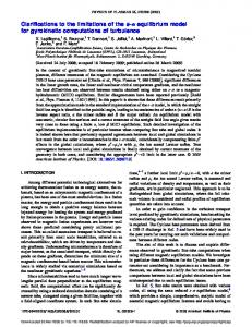
F IGURE 1.1: Grubb curve of the development of a new technology adapted from [27, 82]

The importance of a technology development assessment can be illustrated by assigning the TRLs to the diagram in figure 1.1. It depicts that the TRLs are defined in the phases of research, development, and demonstration in which generally the highest risk of failure and high capital costs impede the technological development. Figure 1.1 outlines the evolution of costs and risks of a technology development from its conceptual design to a state of a mature commercial installation. Such a diagram is often called a ’Grubb’ curve. The grey area embedding the Grubb curve represents the uncertainty of the costs and coherent risks evolving along the development of the technology. It illustrates that in early phases of the development, the underestimation of costs and risks is more prevalent than for phases of deployment and maturity of a technology. Furthermore, the range of uncertainty in the beginning of a technology development is much broader than for later phases. This is the result of learning effects, which also help to reduce the costs and risks in the deployment phase. The given definition of technology development by the DoE [107] defines that combining new and already existing technologies to achieve specific goals is also regarded as technology development. This means that a new process design which may be a combination of new and old process unit technologies is considered to be a technology on its own. It is important to distinguish between a new process design as a technology on its own which generally consists of different process unit technologies and each of the applied process units. They all underlie a 6

certain development from a concept to a mature application. To countervail any confusion, in the following, the term process technology will be applied if a process design is addressed as technology and the term unit technology will be used if a process unit is addressed as technology. The simple use of technology addresses a technology in general. Considering the above, the progress of the process technology development is the result of combining the different TRL of all applied unit technologies, although their development can be at very different TRLs. This is an aspect which has to be considered when comparing results of different process designs in the course of process design & optimisation (PDO) methods. As mentioned in the beginning, the methods of the PSE community are well suited to enhance technology development because they consolidate the scientific knowledge in a single process design & optimisation approach. The consolidation of the attained scientific knowledge in the process design & optimisation tools is essential to narrow down the range of uncertainty about costs and risks of the investigated technology. In the following, the role of the process design & optimisation methodology in the course of the process technology development will be elucidated. The descriptions of TRL 1 to 3 in table 1.1 are elucidating that the conducted work in these TRLs is basically research work on a conceptual basis. It comprises literature review, analytic studies, basic experiments, and basic modelling and simulation. Experiments conducted at TRL 2 are mostly screening experiments designed to corroborate the basic scientific observations made in TRL 1 [107]. The basic concepts and the idea of the process technology are mostly developed in computer aided methods of the PSE community such as the process design & optimisation tool (PDO tool) which will be discussed in chapter 2. The process design is modelled as detailed as possible applying sophisticated models of existing unit technologies. Most of these models apply rule of thumbs, thermodynamic calculations based on equilibrium data or are realised as phenomenological models or 0D models. In these early phases, the uncertainties are rather large since the knowledge about the process and its applied unit technologies is little. Simulations are predominantly simplified because of the lack of data. However, the process design & optimisation in these stages is not highly dependent on data from other groups despite of the data which can be extracted from existing literature. Selection of promising process designs can often already be applied in these stages. Further, the lack of knowledge of the different unit technologies can be identified which allows to suggest experimental work to be conducted to develop the most promising process designs. Within the TRL 3 and 4, experimental work on crucial process steps of the new process designs begins. It entails first laboratory scale experiments which involve data acquisition methods and the generation of first 1D models which are later consolidated to multi-scale rate based models as presented in chapter 3. Experimental planning strategies and parameter estimation come into focus. The experimental effort and capital costs are increasing and the probability that the experimental work is conducted by different groups than the one developing the process designs is high. In fact, it is nearly always the case because scientific needs are

7

Chapter 1. Introduction differing and the scientific expertise is seldom concentrated at only one place. This implies that the concerned research groups may also stay in competition with each other. Within TRL 3 and 4 the unit technology models applied in the process design model should be based on collaborative work to increase the confidence level of these models. The more detailed models are also needed for a improved estimation of process unit sizes and corresponding costs. Furthermore, the integration of the developed multi-scale rate based models in the process design model allows to identify characteristics of the process unit and the process design which otherwise may have been undiscovered. In the course of the technology development of the TRLs 5 to 9 the experimental work is scaled up. This comprises prototypes and demonstrators which allow to validate the model assumptions and to estimate model parameters for operation conditions which are representative for the actual planned operational environment of the technology. The capital costs become a bottle neck of the technology development. Experimental set-ups or demonstration projects have to be carefully planned to avoid disappointments. Attaining experimental data is in most cases highly expensive because the demonstrators on TRL 8 and 9 have already a large scale which elevates the operational costs of an experiment. The process technology development should ideally deliver the questions which have to be tackled during these experiments. The experiments should be focused on process unit characteristics which influence the process design the most. This allows early discovery of possible bottle necks or pitfalls, and a timely search for solutions on either side of the development. Here, the PSE community should seize the opportunity to guide and manage trans-disciplinary research. The models and simulation results attained at TRL 8 and 9 are later often utilised in the final commercial plants for optimisation of operating conditions, and controlling & monitoring purposes. Thus, the process design model of TRL 8 and 9 of the process technology development has to deliver results with a high level of accuracy.

1.1 Motivation In the previous section it has been discussed that the PSE community is acting as a transdisciplinary link between different research fields. The PDO methods of the PSE community consolidate the knowledge of many different research fields in one methodology and therefore depend on experimental based data, detailed models, and on expert knowledge of other research groups. Being dependent on other research groups may be seen as the ’curse’ of the PSE community. However, this interdependency should be seen as an opportunity to guide the development of the alternative unit technologies to a TRL which is needed for a reasonable comparison of the technologies inside the process design. The ultimate vision of the process design model, would be an instantaneously updated process design model where the newest findings and developed models are implemented to build an ideal foundation of the process design & optimisation approach. However, this asks for a well organised and vivid exchange of knowledge between the involved research groups.

8

1.2. Goals and Scope of the Thesis Unfortunately, the reality is that the exchange of expert knowledge (e.g. computer models) does not take place on a short term basis. This has several reasons. The software which is used in the different research groups may differ strongly and compatibility of the methodology and modelling approaches has to be assured. Difficulties in overcoming compatibility issues may hinder an exchange of the developed computer models. Furthermore, the computational infrastructure and the associated calculation time of either of the modelling approaches often counteract a suitable combination of the different modelling strategies. In addition to technical and software specific hindrances, a fear of sharing confidential data may impede the exchange as well. In the context of this thesis the focus will be set on the Wood-to-SNG project. The Woodto-SNG process will be explained in section 2.1. Briefly, in this process, wood is gasified to a syngas which is cleaned from impurities and fed to a methanation reactor where it is converted into a methane rich product gas. The applied process design model was previously developed by EPFL (École Polytechnique Fédérale de Lausanne) . The developed process design & optimisation approach provides the engineers with the ability to simulate and optimise different solutions of a superstructure based process design model by applying a multi-objective optimisation approach based on an evolutionary algorithm. The calculations include the estimation of economic data (i.e. capital costs & operation costs) for which a sound approach of equipment and process unit sizing is needed. A very important process unit in this context is the applied fluidised bed methanation reactor which is in the development and demonstration phase (TRL 7-8). For a sound sizing and scale-up of the methanation reactor, a rate based model which considers the kinetics of the catalyst and hydrodynamic effects has to be used. Such a rate based model has been developed at PSI (Paul Scherrer Institut). It is desired to generate synergies of both technology developments to enhance the development towards a commercial realisation of the Wood-to-SNG project.

1.2 Goals and Scope of the Thesis The goals of the thesis are the following: I the identification of the key elements which are needed to implement a rate based model, such as the fluidised bed methanation reactor model, into the process design & optimisation methodology of EPFL; II the identification and realisation of necessary adaptations on the rate based model according to the identified key elements in (I) to allow its integration into the process design & optimisation methodology; III the realisation of a methodology which helps to limit the increase of computational effort caused by the integration of the rate based model; IV to find programming solutions which allow the process design & optimisation methodology to be applied as originally intended, without the need of applying fundamental 9

Chapter 1. Introduction changes to it. The scope of this thesis project is two fold. The first scope is the integration of the rate based model to enhance the confidence level of modelling results due to a higher level of consolidated knowledge. The second scope is to allow the investigation of the influences of process unit characteristics (methanation reactor) on the process design, and vice versa, more precisely. Especially with the focus on Wood-to-SNG process design options with Power-to-Gas applications (i.e. applying electrolysis to store energy of excess electricity in gas applications) where gas compositions will vary according to the operation conditions and amount of excess electricity. Varying gas composition will have effect on the methane efficiency of the reactor which should be investigated to provide solutions for suitable operation conditions. The targeted approach in this thesis is to develop a surrogate model of the rate based model. Surrogate models are mathematical approximation models based on different mathematical approaches. The most applied and versatile surrogate model types are artificial neural networks, radial basis functions, and Kriging interpolation models. The advantages of surrogate modelling are a shorter calculation time than the approximated computer models, their generalisation capabilities of model results, and the ability to smooth out rough resolution surfaces for faster optimisation results. The developed surrogate model will be implemented into the process design & optimisation methodology of EPFL under the premiss of applying as little modifications as possible to the process design & optimisation models. This should allow the methodology to compute the process designs without interferences of the surrogate model.

1.3 Perspectives Ideally, the investigations in this thesis should allow to apply the here presented approach to any process unit of higher complexity. The advantage in comparison to similar approaches of process design modelling with surrogate models [75, 8, 9, 43, 44] is that not all unit technologies have to apply the surrogate modelling techniques. Where conventional models and short cut models are accurate enough to represent the reality, there is no need for surrogate modelling efforts. With this approach it is possible to selectively apply the surrogate modelling approach to process units which need a higher degree of model detail, but suffer long computation time or are facing software compatibility issues. Furthermore, if the necessary key elements for the integration of the surrogate models are identified, the different research groups are able to prepare surrogate models of the process units and share them with the PSE community in a collaborative environment. Thus, the fear of distributing confidential knowledge should be obsolete and exchange of expert knowledge on timely basis can be targeted.

10

2 Process Design & Optimisation

2.1 Introduction The approach presented in this thesis is based on the work of two former PhD theses. The first is a process design & optimisation methodology developed at EPFL by Gassner [31, 32] which will be presented in section 2.1.2. The other is the work on a rate based model of the fluidised bed methanation reactor developed at PSI [62, 64] which will be described in chapter 3. Both theses have been prepared in the context of the Wood-to-SNG process. For a guidance the following section will introduce the reader to the Wood-to-SNG process followed by an introduction into the afore mentioned process design & optimisation methodology.

2.1.1 The Wood-to-SNG Process Figure 2.1 depicts the four general process steps of the Wood-to-SNG process. Depending on the applied gasification technology, wet or dried wood is fed to the gasification unit which converts the wood under addition of a gasification agent (air, oxygen and/or water steam) into the so called producer gas. This gas consists mainly of H2 , CO, CO2 , H2 O, CH4 , C2 H4 , and if the gasification agent is air N2 as well. Additionally, impurities like small amounts of sulphur compounds, olefins and tars are gasification products. Most of these compounds harm the catalyst in the subsequent methane synthesis (methanation) step. They either cause deactivation of the catalyst by irreversible adsorption on the active sites (sulphur) or by carbon deposition. Therefore, a gas cleaning step is necessary. Well established cold gas cleaning (scrubbers) or more advanced catalytic hot gas cleaning are possible technology options. While the former can be categorised as a mature technology, the latter may be labelled with TRL 7, i.e. it is still in the phase of development & demonstration. In any case, both technologies are applied in combination with additional guard beds (Cu + ZnO) to protect the more expensive methanation catalyst. In the subsequent synthesis step, methane is formed from CO and H2 in the exothermic methanation reaction utilising a suited methanation catalyst (usually nickel based). The methanation step considered in this thesis is an isothermal bubbling fluidised bed methanation reactor. An alternative technology option would be a series of catalytic fixed bed 11

Chapter 2. Process Design & Optimisation

Heating & Cooling Infrastructure (Energy Integration Calculations)

Gasification Autothermal Producer Gas

Wood

Gas Cleaning

Methanation

Gas Upgrading

Cold gas Cleaning

Bubbling Fluidised Bed

Physical absorption (scrubbers) Pressure Swing adsorption

Allothermal

Warm Gas Cleaning

Catalytic Fluidised Bed . . .

Hot Gas Cleaning . . .

Clean Raw Gas

Raw SNG Fixed Bed . . .

SNG

Membranes . . .

F IGURE 2.1: Alternative process unit technologies for each step of the Wood-to-SNG (Synthetic Natural Gas) process with illustration of the energy integration system.

methanation units with intermediate cooling and product gas recirculation to dampen the temperature rise in the fixed bed reactors. The last process step is a gas upgrading step which adjusts the gas mixture according to the required gas quality for an injection into the natural gas grid. The injection is regulated by national associations by providing the required range of the Wobbe Index. The Wobbe index is an indicator for the interchangeability of combustion fuel gases. The definition of the Wobbe index is given by eq. (2.1) in section 2.3. In this step mainly CO2 and H2 O are separated from the gas stream. Additionally, excess hydrogen is recovered and fed back to the feed of the methanation step or may be used to cover part of the energy demand of the process via combustion. For further detailed technology review please refer to Kopyscinski et al. [63]. The list of technology options presented in figure 2.1 is exemplary and by no means exhaustive.

2.1.2 The Process Design & Optimisation Methodology The process design & optimisation methodology developed by Gassner and Maréchal [32] combines a process design model with a model for mass and energy integration calculations based on a predefined superstructure for the purpose of evaluating and optimising process designs using a multi-objective optimisation strategy. In the following, this approach will either be called the process design & optimisation (PDO) methodology or the PDO procedure. The required software tools are going to be called the PDO framework or the PDO tools. Figure 2.2 illustrates the flow of information in the computational procedure when applying the PDO methodology. It depicts that the PDO framework utilises an evolutionary optimisation algorithm which applies a set of models referred to as the process design model. The process design model consists of thermodynamic models which are calculating mass & energy balances and the thermo-economic models which are calculating process unit sizes based on the thermodynamic models and deducing the investment costs of the process design from 12

2.1. Introduction

F IGURE 2.2: Computational and information flow diagram of the process design & optimisation framework.

this knowledge. As Gassner and Maréchal [32] describe, the PDO methodology is based on the decomposition of the thermodynamic models into two parts. The decomposition into two parts corresponds to the models which are denoted as the non-linear and the linear problem in figure 2.2. The non-linear problem comprises the process flowsheet modelled in a commercially available software and the linear problem comprises a heat cascade model which is used in the pinch point analysis of the process design. The application of the PDO procedure is applied as follows. The process engineers conduct a pre-selection of possible process designs and unit technology options to define the superstructure of the process design model (see figure 2.3 in section 2.2). The applied process superstructure consolidates the different technologies and their possible interconnections. The technologies and mandatory auxiliaries as well as feed, product, and recycle streams are defined in the process superstructure. The use of a process superstructure implies that integer decision variables have to be defined prior to the thermodynamic calculations. The integer decision variables are activating and deactivating given substructures (i.e. technologies or combinations of technologies) in the superstructure. The corresponding decision variables 13

Chapter 2. Process Design & Optimisation are programmed into the non-linear and the linear problem statements. Together with the integer decision variables the process model forms a mixed integer non-linear programming (MINLP) problem which is addressed to the multi-objective optimisation (MOO) procedure. The superstructure builds the foundation of the applied MOO procedure. The MOO procedure will allow to identify the most promising concepts out of the proposed ones with respect to conflicting objectives. These objectives are also preceding information which has to be defined by the engineers. The decision variables are set in the course of the evolutionary multi-objective optimisation. They are defined previous to each iteration of the evolutionary algorithm. The decision variables differ from one generation of process designs to another. Each set of decision variables is an unique attribute of the resulting process design which allows to recalculate certain process designs if values of the applied decision variables are known. Process streams are generally defined by a combination of extensive and intensive properties. Extensive properties are those which can be added up if two streams are mixed, e.g. mass flows and energy flows. Intensive properties are those which in the given case do not allow to be added up, e.g. temperature, pressure, and weight fractions. The applied process superstructure has a special feature regarding the process streams defined in the commercial flowsheeting software which are connecting the different technologies. In the case of the connecting process streams only the intensive state variables of the process streams are linked with each other; i.e. the temperature, pressure, and weight fractions of an output stream of one unit technology are passed to the input stream of the subsequent unit technology. The extensive variables are treated separately and are not linked with each other. Instead, the main input stream of each kg of the technologies in the superstructure is set to a mass flow of 1 s . The mass flows of other input streams of a unit technology are set in relation to this main stream. Therefore, all streams defined in a unit technology, including flows of heat and power, are easily scalable by only one factor. The resulting mass and energy flows of the process flowsheet model (non-linear) are denoted as normalised extensive state variables in figure 2.2 since they are always related kg to a main input of 1 s . They are passed to the mass & energy balances defined in the linear problem where they are applied to a heat cascade model. In the following, the linear problem will be called energy integration model, although it solves a combination of mass & energy integration. The energy integration model calculates scaling factors for each technology during the mass & energy integration calculations based on a pinch point analysis of the heat cascades. Consequently, it defines the final mass & energy flows of the process design. The targets of the energy integration calculations are a minimal use of heating & cooling utilities and maximum production of the desired product stream. A pinch point analysis is applied to support the energy integration calculations. After the calculation of the thermodynamic states, the thermo-economic properties of the evaluated process design are computed in a so called post-processing step. The post-processing step determines the sizes of the process units in dependence of the final results of the extensive and intensive variables calculated in the thermodynamic models. The performances of the process design and the objectives needed in the multi-objective optimisation algorithm are 14

2.2. Background also calculated in this post-processing step. These are for example, thermodynamic efficiencies, capital costs, costs of operation and maintenance, and life-cycle assessment ratings. The calculated objectives of a selection of evaluated process designs are finally plotted in a graph. The optimisation procedure will drive the results to a pareto frontier which is updated on every iteration of the optimisation process. Ideally, the progress of the pareto frontier will be examined and if only very little improvements are made between the different iterations, the optimisation process is stopped. In the current solution a certain number of iteration steps is specified after which the calculation will stop and the improvements are visually examined. Finally, the engineers have to check the quality of the solutions and disqualify solutions which do not make physical sense.

2.2 Background The above described process design & optimisation methodology has been applied to study the Wood-to-SNG process in [31, 33]. Gassner and Maréchal [33] developed a superstructure based process design model to investigate the Wood-to-SNG process with the afore described multi-objective optimisation methodology. The corresponding superstructure is illustrated in figure 2.3 and considers seven subsystems which are: • Drying (of the biomass) • Thermal Pretreatment (of the biomass) • Gasification • Gas Cleaning • Synthesis Preparation (also referred as gas conditioning) • Methane Synthesis • SNG Upgrading • Utility and Heat Recovery System Each of these subsystems includes a certain number of alternative unit technology models which are combined to an applicable process design by presetting decision variables of the superstructure. A central subsystem is the methane synthesis step. The fluidised bed methanation reactor which is one of the considered technology options is developed at PSI. The properties of the gas feed of the methanation reactor together with the hydrodynamic properties of the fluidised bed are the major concern of the engineers developing the fluidised bed methanation technology. Impurities like sulphur compounds, tars, olefins and inorganic contaminants are causes of catalyst deactivation. A not less important aspect are the bulk compounds in the gas 15

F IGURE 2.3: Process superstructure developed by Gassner and Maréchal [33] including main process streams without recycling loops. Groups of technology alternatives for the defined process subsystems and additional optional process units are illustrated. Reprinted from Gassner and Maréchal [33], Copyright (2009), with permission from Elsevier

Chapter 2. Process Design & Optimisation

16

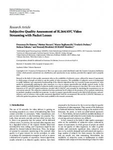
2.2. Background feed because they may have significant influence on the outcome of the chemical reaction system. Investigation at PSI dealing with the application of the fluidised bed methanation in the Wood-to-SNG process raised the question how the choice of the gas cleaning technology would influence the performance of the fluidised bed methanation reactor. The considered gas cleaning technologies are the cold gas cleaning (i.e. absorption process in a scrubber) or a catalytic hot gas cleaning (i.e. a reactor equipped with a catalytic monolith) as figure 2.3 depicts. Despite of the differing technology readiness levels (TRL’s) of these two technologies (catalytic hot gas cleaning at about TRL 7, cold gas cleaning a mature technology), the major concern was the influence of the water content on the performance of the fluidised bed methanation reactor. In contrast to the hot gas cleaning, the cold gas cleaning approach removes a significant amount of water from the gas stream. Applying the cold gas cleaning, the water content in the methanation feed can be adjusted to a desired value just before fed to the methane synthesis step by steam addition. If the hot gas cleaning is applied, the methanation has to deal with the rather high water content which leaves the gasification unit. It should be noticed that the fluidised bed methanation reactor in the original superstructure implemented by Gassner and Maréchal [33] was realised based on the assumption of thermodynamic equilibrium of the considered reaction system. This assumption was based on laboratory scale experimental knowledge attained at PSI which was later published by Seemann et al. [89]. These experiments where conducted at a relatively high reaction temperature around 385 ◦C and 400 ◦C. Due to the lack of knowledge, it was assumed to extend the assumption of thermodynamic equilibrium to the full temperature range. Meanwhile, the developments in the research on the fluidised bed methanation reactor have reached a state where a suitable rate based model with experimental data at its foundation is available (see [65, 64]). This rate based model is topic of chapter 3. As figure 2.4 shows, the new model has the clear potential to improve the current methanation model applied in the process design model. The illustrated surface in figure 2.4 represents the results of the thermodynamic equilibrium model and the pictured data points are calculations of the rate based fluidised bed model. The graph demonstrates that the assumption of thermodynamic equilibrium is applicable unless the reaction temperature falls under 330 ◦C. Figure 2.4 furthermore shows that there is a superimposing effect of the reaction temperature and the initial water content on the total CO conversion. With increasing water content the total CO conversion decreases. This effect becomes stronger with lower temperature. It is obvious that the use of the thermodynamic equilibrium would not allow the analysis of these effects on the process design. To allow a more accurate representation of the fluidised bed methanation reactor at a temperature lower than 330 ◦C the use of the rate based model is required. The above presented aspects emphasise that there is a need to consolidate the attained knowledge (experimental & modelling knowledge) about the fluidised bed methanation reactor with 17

Chapter 2. Process Design & Optimisation

Total CO Conversion

Thermodynamic Equlibrium vs. Rate Based Model

0.98 0.96 0.94 0.92 0.9 0.88 0.86 400

350

Fluidised Bed Tempera ture [ ◦C]

300

0

3 2 l H 2O 1 Initia f o w CO r Flo itial Mola of In w o l rF Mola

F IGURE 2.4: Comparison of the thermodynamic equilibrium model (coloured surface), and the rate based fluidised bed model (data points) for varying temperature and H2 O to CO ratio.

the PDO methodology to allow further process technology development of the Wood-to-SNG project.

2.3 Process Design Model for the Case Study In the following, a sound basis for investigating the effects on the process design caused by the integration of the new fluidised bed methanation model will be presented. A process design without applying the optimisation procedure will be defined as case study to investigate the effects under controlled conditions. However, the applied changes as well as the implementation of the rate based model are conducted with respect to support a future application of the optimisation procedure. The case study is based on the superstructure presented above (see figure 2.3). The integer decision variables, which are controlling the activation of the different process technologies of the superstructure, are set a priori to fix a specific process design for the case study. Table 2.1 lists the chosen technologies for each of the in figure 2.3 defined subsystems. Figure 2.5 illustrates the resulting process flowsheet. The main feed of the process design is wet biomass which is fed to the air dryer. The dried wood is subsequently fed into the Fast Internally Circulating Fluidised Bed (FICFB) gasifier where it is gasified utilising steam. The producer gas has to be cleaned from tars and sulphur compounds. Since these compounds are not represented in the model, a gas cleaning step would not have to be considered. However, the temperature change of the main gas stream and possible changes in the composition of the bulk compounds have to be considered. The chosen gas cleaning step is a cold gas scrubbing unit with biodiesel (RME) as scrubbing liquid. The cold gas scrubbing reduces the water 18

2.3. Process Design Model for the Case Study TABLE 2.1: Applied technologies for the different subsystems of the Wood-to-SNG process design. Subsystem

Applied Technology

Drying

Air Dryer

Thermal Pretreatment

deactivated

Gasification

Indirectly Heated Steam Blown Gasification (e.g. FICFB)

Gas Cleaning

Cold Gas Cleaning (scrubbing + Cu & ZnO guard beds )

Synthesis Preparation

deactivated

Electrolysis

activated

Methane Synthesis

Internally Cooled Fluidised Bed Methanation

SNG-Upgrading

Temperature Swing Adsorption (TSA) SELEXOL™ CO2 seperation Polyimide (Matrimid) Membrane for H2 -recovery

Utility and Heat Recovery System

no application of Rankine cycles

content in the gas stream significantly. However, to reduce the risk of carbon deposition on the methanation catalyst, a certain amount of water is required in the feed of the methanation reactor. Therefore, steam is added to the methanation reactor feed. After the methanation, water has to be removed before the gas is fed to the SELEXOL™ absorption process. In the last process step, the hydrogen content is reduced via membrane separation. As figure 2.5 depicts, the permeate is recycled to the methanation reactor feed. A very important and restrictive decision variable of the process simulation is the Wobbe index of the final SNG. The Wobbe index is defined as the ratio between the volumetric higher heating value and the square root of the relative gas density d v . The relative gas density d v is defined by the ratio between the combustible gas density and the density of air at 0 ◦C and 101.325 kPa. The definition of the Wobbe index is given by eq. (2.1). Wv,HHV =

HHVv (298.15 K) p dv

kW h m3std.

(2.1)

Further information and definitions are given in [20]. In the assumptions of the original process design model the ethylene produced by the gasifier was converted completely to methane by the methane synthesis step. Experiments have shown that a considerable amount of ethylene is actually converted into ethane. Currently, there are no kinetics developed at PSI to estimate the amount of ethane produced. However, it was decided to consider ethane as an additional compound in the SNG stream since it has considerable influence on the Wobbe index. It is assumed that the fluidised bed methanation reactor converts half of the ethylene in the feed stream into ethane and the other half into 19

Chapter 2. Process Design & Optimisation Electrolysis H2 O

Wel

Exhaust Gas

Condenser +TSA

Air

SNG

State C

CO2

State A

H2 + CO2

Steam

Air

H2 -Recovery

H2 SELEXOL

FAME

Biomass

State B

H2 O

Steam Drying

Gasication

Gas Cleaning Methane Synthesis

SNG-Upgrading

F IGURE 2.5: Process flowsheet diagram of the Wood-to-SNG process design illustrating the defined case study.

methane. In comparison to the original process superstructure, the gas upgrading system had to be partly changed. The definition of ethane as additional compound is one of the reasons why the gas upgrading system had to be revised. The addition of ethane introduced some convergence issues when solving the process flowsheet. The major cause is the influence of the ethane content on the value of the Wobbe index. The figure 2.6 illustrates the relation between the composition of a given gas and its Wobbe index. Towards the upper left corner of the graph, high Wobbe indices are located. Towards the lower right corner, low Wobbe indices are located. Six red dots are marking the location of the pure compounds in the graph. Furthermore, three mixing lines indicate the possible positions of binary mixtures between CH4 & C2 H6 , CH4 & H2 , and CO2 & H2 . The national gas grid carriers have published regulations defining the gas properties which have to lie in certain limits for injection into the national natural gas grid. The limits of the Wobbe index, the volumetric higher heating value, and the relative gas density set by the German Gas and Water Industry Association (DVGW) [22] for H-gas quality are represented by the coloured area in figure 2.6. The smaller area bordered by the black dash-dotted line represents the corresponding limits set by the Swiss Gas and Water Industry Association (SVGW) [103]. As the graph shows, the regulations do not only consider the Wobbe index, but also approved limits of the relative density and higher heating value in which the gas mixture has to lie. Furthermore, upper limits of volumetric fractions of many compounds are regulated. For example, a maximum of 20

2.3. Process Design Model for the Case Study TABLE 2.2: Solubility of selected compounds in SELEXOL, adopted from [104, 7].

Solubility of CO2 a ~0.004

H2

m3std.

0.013

lsolvent

a adopted from [104]

Solubilities of Gases Relative to CO2 b N2 CO CH4 C2 H6

H2 O

0.020

730

0.028

0.066

0.42

b adopted from [7]

4 vol% of hydrogen, a minimum of 96 vol% of methane, and a maximum of 6 vol% of CO2 are permitted. Therefore, the last steps of the process – the methanation, the SELEXOL scrubber, and the hydrogen recovery membrane – have to be adjusted such that the SNG quality hits the strict injection criteria. Figure 2.6 pictures black dots which are representing three states of the main process gas stream along the gas upgrading steps. The three states along the process chain are the input stream of the SELEXOL subsystem (state A), its output stream respectively the input stream of the hydrogen recovery membrane (state B), and the final SNG product stream (state C). These states are plotted for three different molar stage cuts θs of the hydrogen recovery membrane. The stage cut of a membrane defines the ratio between the molar flow of the permeate and the molar flow of the retentate. The amount of permeate is increased by a larger membrane area, a higher differential pressure, and a higher permeability of the membrane for the corresponding compounds. Two other mixing lines, a dash-dotted line (blue) and a dashed line (magenta) which are representing the gas separation in the SELEXOL CO2 -separation and the H2 -recovery membrane, respectively, are plotted in figure 2.6.

SELEXOL CO2 -separation The dash-dotted line (blue) connects the state A with the point of pure CO2 . Following the line from the gas mixture of state A towards the point of pure CO2 is equivalent to an addition of pure CO2 . Following the line in the other direction implies separation of pure CO2 . Hence, the number of theoretical stages of the absorption column increases, the further the quality targets of the gas mixture are shifted towards the upper left of the graph. The separation of CO2 by the SELEXOL scrubbing system — depending on which stage cut has been applied — results in the three gas mixtures marked as state B. As figure 2.6 illustrates, the points of state B slightly deviate from the mixing line which connects state A and the point of pure CO2 . Unfortunately, the solubility of ethane in SELEXOL lies between those of CH4 and CO2 , see table 2.2. According to Burr and Lyddon [7], the relative volumetric solubility of ethane and methane to carbon dioxide in SELEXOL are 42% and 6.6%, respectively. The applied operation conditions of the SELEXOL gas absorption process have to ensure a high recovery factor for methane while maintaining a high separation factor for CO2 . The gas absorption system is calculated utilising the Kremser equation [19] and the assumption of an 21

Chapter 2. Process Design & Optimisation TABLE 2.3: Gas permeabilities of polysulfone and polyimide (Matrimid) membrane material used for industrial gas separation applications, adopted from [1] and [85].

Material

H2

Polysulfone Polyimide (Matrimid) ·

a 10−9

cm3 cm cm2 s mmHg

¸

14 28.1

Permeability at 30 ◦C in Barrera N2 O2 CH4 CO2 0.25 0.32

1.4 2.13

b not applied in the original process design model

0.25 0.25

5.6 10.7

C2 H6 —b ~0.1c

c adopted from [85]

average absorption factor calculated via eq. (2.2). A CO2 =

L0 , K CO2 · VN +1

(2.2)

where L 0 represents the molar flow rate of the lean solvent, VN +1 represents the molar flow rate of the CO2 -rich feed gas of the absorber column, and K CO2 = y/x represents the slope of the linear assumed vapour-liquid equilibrium line. For detailed description of the applied gas absorption estimation in the SELEXOL gas absorption process, please refer to [19] where a simplified equation for absorber performance based on the work of Souders et al. [97] is presented. Furthermore, Gassner [31] described the approach implemented in the process design model.

H2 -recovery The dashed line (magenta) in figure 2.6 starts from a point on the H2 & CO2 mixing line and connects it with the gas mixture of state B which corresponds to a stage cut of θs = 0.15. The point on the H2 & CO2 mixing line represents a gas mixture which corresponds to the selectivity of the applied Matrimid® membrane. In the original process design model a polysulfone membrane was applied. However, during the adaptation of the gas upgrading system it was found that a higher H2 /CH4 selectivity for the hydrogen recovery membrane was required and therefore polyimide (Matrimid) membrane was chosen. The membrane permeabilities of the Matrimid membrane are adopted from [1] and [85] and are compared to the polysulfone material in table 2.3. The afore mentioned dashed line illustrates a theoretical separation of a hydrogen and carbon dioxide mixture from the process stream corresponding to the selectivity of the membrane. It has to be noticed that both separation lines, the dashed kW h and the dash-dotted line, end in a region with Wobbe index of about 14.5 m 3 . In this example, std.

this is the calculative state of complete H2 and CO2 separation. Hence, it is the point of infinite membrane area and infinite number of theoretical stages of the absorber column. It is obvious that the separation systems are heavily utilised for reaching the needed specifications because the gas mixture of state C is very close to the point of complete H2 & CO2 separation. Thus, kW h attaining a Wobbe index of 14.5 m is challenging. The Wobbe index of pure methane has a 3 std.

kW h value of about 14.85 m 3 . In this context, higher values can only be reached with addition of

ethane. 22

std.

Volumetric Higher Heating Value HHVv in

0

0.2

0.4

0.6

Relative Density

0.8

dv

1.0

2 1.2

1.4

2

CO

1.6

13

13.5

kW h m3std.

F IGURE 2.6: Influences of gas composition and process unit operations in the Wood-to-SNG process on a measure of gas quality, the Wobbe index.

kW h m3std. N

CO

H2 - CO2 Selectivity of the Matrimid Membrane

14

in

0

H2 & CO2 mixing line

State A

Before Selexol Scrubbing

14.5

v

2

2

H

Separation of pure CO2

State B

After Selexol Scrubbing & before H2 -Separation Membrane

15

15.5

dv

4

θs = 0.2

θs = 0.15

θs = 0.1

State C

Final SNG Product

2 6

C H

p = HHV

6

CH4 & H2 mixing line

4

CH

CH4 & C2 H6 mixing line Volumetric Wobbe Index Wv

8

10

12

14

16

18

20

2.3. Process Design Model for the Case Study

23

Chapter 2. Process Design & Optimisation Gas Separation Systems in Interaction The position of the process streams at state C inside the marked area of the SVGW is defined a priori by setting a decision variable which fixes the kW h Wobbe index of the SNG to 13.5 m 3 . How this stage is reached depends on the choice of the std.

membrane stage cut. Since the pressure difference over the membrane and its permeability are fixed, the stage cut defines the size of the membrane area. Figure 2.6 illustrates, that an increase of the stage cut of the hydrogen recovery membrane (increase of membrane area) reduces the amount of CO2 which has to be separated by the SELEXOL scrubbing system. This is indicated by the position of the gas mixtures of state B. A higher stage cut shifts the gas mixture of state B closer to the gas mixture of state A. This stands for an increased separation load of the membrane which implies that larger investment costs have to be made. However, the investment into the membrane area means that the system becomes more inflexible which raises the question which solution will be the most advantageous one. In this case, the use of a process design & optimisation tool reveals its advantage. Since the engineers decision about the stage cut of the membrane has to be made a priori to calculate the process flowsheet, the evolutionary optimisation approach will easily apply the search for the best stage cut. Because the process operates already at the lower limit of the targeted Wobbe index, a slight variation of the decision variables may lead to convergence issues of the process simulation. A miscalculation of the Wobbe index by 25% in the original version of the process design model had caused such resolution problems after ethane has been introduced into the process streams.

2.3.1 Adaptations to Support Future Process Optimisation Two additional features have been introduced to the process design model to support future process optimisation. The two features are located in the SNG-upgrading subsystem. The first is a revision of the compressor which re-compresses the gas of the SELEXOL flash for recirculating it to the feed of the absorber column (stripper column and recompression not illustrated in figure 2.5). This recirculation accumulates the less soluble gases in the loop to increase the recovery rate in the main outlet of the absorber column. Since the pressure difference between absorption and regeneration of the SELEXOL may later be subject of p optimisation and the corresponding pressure ratio absorber p flash may be rather high, the applied compression system was revised. The revision allows a more realistic representation of the amount of heat and power utilised and of the temperature at which the heat streams are available. The original representation of this compression was a single stage compressor which resulted in available heat at high temperature after the compressor if a large compression ratio was required. Ulrich and Vasudevan [108, p. 158] state that for a compression ratio larger than a factor 4 the compression units must be staged. With compression ratios 4 and larger the isentropic discharge temperature of a diatomic ideal gas reaches 200 ◦C. Temperatures higher than that can cause serious damage to lubricants, seals, and other sensitive materials [108, p. 158]. Therefore, an integrated selection between a 1-stage, 2-stage, and 3-stage

24

2.3. Process Design Model for the Case Study compression solution with intermediate cooling has been modelled as illustrated in figure 2.7. This will improve the confidence level of the heat integration calculations because in a 3-stage compression system, the total amount of heat is available at a lower temperature than in p a single stage compression system. Depending on the pressure ratio r p = pout , one of the in compressor lines is utilised so that each compressor has a maximum compression ratio of factor 4. Two stream splitters (S1 and S2) split the input stream depending on which pressure ratio is requested. The split fractions s 1 and s 2 are defined by eq. (2.3), respectively. To allow a smooth transition similar to a rapid switch between two technologies, a transition factor f tr is applied. This transition factor is dependent on the difference between the desired pressure ratio and the actual pressure ratio ∆r p = r p,desired − r p .

s = f tr · 0.9999 + 0.00001 =

erf(70 · ∆r p ) + 1 2

· 0.9999 + 0.00001

(2.3)

The factor 70 in eq. (2.3) controls the width of the transition range observable in figure 2.7. Increasing this factor reduces the width of the transition and decreasing the factor widens the transition. For the split fraction s 1 the desired pressure ratio is set to 4 and for the split fraction s 2 it is set to 16. This means that unless the pressure ratio exceeds the factor 4, the single compressor line is the utilised. If it exceeds the factor 4 and is lower than 16, the 2-stage compressor line is the main compression route. For every pressure ratio larger than 16, the 3-stage compressor line is used. According to eq. (2.3) the split factor has a minimum of 0.00001. Consequently, all three compressor lines are actually utilised simultaneously. However, two of the three lines are operated with a very low mass flow so that they have only negligible influence on the final result. Economic calculations may be applied in correspondence to the primarily utilised compression line. The presented solution of the 3-lane compression system may be generally applied to all process streams which require a compression over a large pressure range. The second feature which was implemented into the superstructure concerns the pressure adjustment of a subsystem’s feed stream. The applied solution is an integrated pressure adjustment of the gas upgrading system’s feed stream. This feature utilises a combination of a compressor and a pressure release valve, see figure 2.8a. To illustrate the reason of this implementation one has to recall that the superstructure is an independent set of process unit models. If an output of one unit model has to be combined with the input of another, the intensive variables such as temperature and pressure are passed from the output to the input stream. This takes place independent of whether the pressure of the first process unit is lower than the pressure of the second process unit or higher. Thus, a pressure and a temperature correction has to be applied on every input stream, so that the required temperature and pressure in the corresponding unit technology can be guaranteed. A temperature correction via a heat exchanger was previously already applied. Also a pressure adjustment was considered, however, only a compressor was utilised. Situations in which the outlet pressure of 25

Chapter 2. Process Design & Optimisation

rp ≤ 4

S1

p in rp > 4 r p ≤ 16

S2

r p > 16

1

1

Transition Factor f tr

0.8

0.8

0.6

2

1−(

0.4 0.2

p

r p = pout in

erf(70·∆r p )+1

2

)

0.4 0.2

0 -0.1 -0.08 -0.06 -0.04 -0.02 0

M1

0.6

erf(70·∆r p )+1

0 0.02 0.04 0.06 0.08 0.1

∆r p = r p ,desired − r p

p out

(a) Process flowsheet of the 3-lane compres- (b) Transition factor for smooth transition between two comsion system. pressor lines. F IGURE 2.7: Application of a self-adjusting 3-lane compression system which applies a 1-stage, 2-stage, or 3-stage compression line.

the previous subsystem is higher than the required pressure in the subsequent subsystem were previously not handled in an integrated manner. The pressure had always to be adjusted in a pre-computation step which required to know the outlet pressures of previous process units a priori. Thus, the pressures in the corresponding streams had to be defined as decision variables. This is detrimental if pressure drop equations are going to be implemented in the future. The combination of a compressor and a valve in series is suitable concept to avoid the described issue. Figure 2.8a illustrates the solution which should be applied to adjust any input of a subsystem in the superstructure. It depicts the use of a compressor operated in series with a pressure release valve and a heat exchanger. Ideally, the depicted single compression stage may be exchanged with the above presented 3-lane compressor system if large pressure ranges are expected. Figure 2.8b depicts how a transition between pure pressure relief and compression is achieved. To allow a smooth transition the pressure p m of the middle stream between the compressor and the pressure relief valve is evaluated in dependence of the applied pressure difference ∆p = p set − p in , see eq. (2.4).



∆p pm =  + 2

26

s

µ

∆p 2

¶2



+ 0.0005 + p in = p adj + p in

(2.4)

2.4. Conclusions

0.6

p in

=

p

se

t

0.4

m

0.3

p

pm

p adj = p m − p in (bar)

0.5

0.2

0.1

parity line

p m = p in p set (a) Scheme of the input stream pressure adjustment.

0 -0.5 -0.4 -0.3 -0.2 -0.1

0

0.1

0.2

0.3

0.4

0.5

∆p = p set − p in (bar)

(b) Graph representing the development of the intermediate pressure between compressor and pressure release valve in dependence of the desired pressure difference.

F IGURE 2.8: Example of a flexible and generally applicable input stream pressure adjustment for subsystems in a superstructure based process design model.

Both new features increase the flexibility of the applied superstructure while avoiding the introduction of new integer decision variables. Keeping the number of integer decision variables low, reduces the number of evaluations during the evolutionary optimisation approach because less integer variables have to be combined with each other. It also reduces the risk of attaining ill-conditioned process designs which would have to be rejected in a final step.

2.4 Conclusions This chapter gave an introduction to the process design & optimisation methodology applied and developed at EPFL. Further, the Wood-to-SNG process was presented which stakes out the frame in which this thesis has been developed. A sound basis of a process design model was presented for a case study investigating the integration of a rate based model (fluidised bed methanation reactor model). The experimental experiences and the developed methanation kinetics as well as the fluidised bed methanation reactor model at PSI emphasise the need to further improve the representation of the methanation model embedded in the existing process design model. Larger deviations at low temperature between the results of thermodynamic equilibrium and the developed rate based model further indicate this need. A revision of the process design model has been conducted to allow the later integration of the rate based model into the process design model and required adaptations were made. These were the consideration of ethane in the process flows and the necessary adaptations to the SNG upgrad27

Chapter 2. Process Design & Optimisation ing system to be able to deal with this compound. Furthermore, with the goal in mind of using the final process design model with integrated rate based model in an optimisation procedure, two new modelling solutions for pressure adjustments in process streams were presented. The two modelling solutions are a 3-lane compressor system and a compressor valve combination with sophisticated transition functions to allow smooth transitions between different states. With these adaptations of the original process design model, a foundation is set to begin a comparison of the process design characteristics and performances of the solution with integrated rate based model and with thermodynamic equilibrium under controlled conditions. The next necessary steps are the revision of the rate based model to make it applicable to the process design & optimisation procedure, the development of its surrogate model, and the integration of the surrogate model into the process design & optimisation methodology, respectively to the process design model.

28

3 The Rate Based Model

This chapter is based on the manuscript of Sinan L Teske, Jan Kopyscinski, Tilman J Schildhauer, Simon Maurer, and Serge M A Biollaz. “Validating a Rate Based Model of a Fluidised Bed Methanation Reactor”. In: Manuscript in preparation (2013) J. Kopyscinski contributed by identifying the parameters for the new kinetics 3m and by contributing to the discussions about the measured concentration profiles in the lab-scale fluidised bed experiments. S. Maurer contributed by supporting the experiments on the bubble hold-up described in section 3.2.2 and providing figures 3.2a and 3.2b. 29

Chapter 3. The Rate Based Model This chapter describes the rate based model of the bubbling fluidised bed reactor, which is the object of later surrogate modelling and incorporation into the process design & optimisation tool. It describes the original model and the adaptations and implementations which are necessary for its later implementation.

3.1 Introduction Catalytic fluidised beds are extensively used in gas-solid applications in which large heat and mass transfer rates are required. The methanation of syngas with a high CO partial pressure is an example of a fast and highly exothermic reaction eq. (3.1). It has been shown that a catalytic fluidised bed reactor is well suited for the conversion of biomass derived producer gas to synthetic natural gas - SNG [63, 89]. Fluidised bed reactors allow for an isothermal one-step operation combining the methanation eq. (3.1) and water gas shift eq. (3.2) reaction. In addition, the movement of the catalyst particles through the bed enables long catalyst stability due to internal regeneration [61].

−−− * CO + 3 H2 ) − CH4 + H2 O −− * CO + H2 O − ) − CO2 + H2

kJ mol kJ 0 ∆HR = −41 mol ∆H0R = −206

(3.1) (3.2)

A common approach for engineers in process systems engineering to describe process steps with little or no information is to state the assumption of chemical equilibrium. Thus, maximum theoretical efficiencies and trends (e.g., influence of temperature) can be predicted, however, economic calculation including reactor design might lead to over-optimistic estimates. Especially in multiphase reactors such as fluidised beds, aspects of kinetics, hydrodynamics, and mass transfer influence the reactor performance, reactant conversion, and product selectivity [62]. Therefore, a detailed rate based reactor model is desired for application in process modelling and optimisation methodologies as described in chapter 2. The aim of the work described in this chapter is to check the performance of the rate based model in predicting real world experiments in fluidised bed methanation reactors as they were conducted in earlier stages of the fluidised bed methanation development. In the experimental runs, the partial pressure of the reactants, the volume flow, the catalyst hold-up, and the catalyst dilution were changed. Furthermore, challenges of using axial gas profiles to judge prediction performance of the rate based model are discussed.

30

3.2. Background & Model Revision

3.2 Background & Model Revision 3.2.1 Lab-scale Fluidised Bed Experiments The experimental set up and procedure have been described in detail in [67]. The setup consisted of mass flow controllers, heated gas lines, a fluidised bed reactor (52 mm inner diameter), a filter, a condenser, and online gas analysis, see figure 3.1.

Step motor

Gas sampling Catalyst sampling

T-probe

Cooling Agent

T-bed

Thermocouples and probe tip

Syngas

Fluidized bed F IGURE 3.1: Scheme of the experimental set-up of the fluidised bed methanation (left) and a scheme of the definition of the one dimensional molar balance (along the reactor height) of the two phase fluidised bed model (right). Adapted with permission from Kopyscinski et al. [68]. Copyright (2014) American Chemical Society.

The reactants are fed into the fluidised bed through a non reactive porous metal plate distributor. The product gas leaving the reactor was condensed and sent to the fume hood. The spatially resolved gas composition and temperature profiles were acquired with a moveable sampling capillary connected to an online micro gas chromatograph (Varian Model CP 4900; detector TCD, Columns MSA5, PPU). The amount of produced water was measured by weighing the condensed water after the reactor, taking the gas humidity after condensation into account. Depending on the catalyst loading and the gas volume flow, the bed heights varied between 65 and 190 mm. The experimental conditions are summarised in table 3.1, of which numbers 1 to 10 have been presented in [67]. An additional experiment (#11 in table 3.1) was conducted in which 20 g catalyst was diluted with 80 g of alumina. All experiments were performed at 320 ◦C varying the chemical space velocity (CSV) by dilution with nitrogen or by dilution of the catalyst with alumina. Further details to the performed experiments can be found in [67]. 31

Chapter 3. The Rate Based Model TABLE 3.1: Settings of the laboratory fluidised bed experiments

No.

1 2 3 4 5 6 7 8 9 10 11

Mass

P

H2

N2

CSV(CO)

gcat

lN ·min−1 (inlet flow)

gCO ·min−1 ·kg−1 cat

70 100 140 200 100 200 70 100 200 100 20*

10 10 10 10 14 14 8.1 8.1 8.1 16.2 10

6.0 6.0 6.0 6.0 8.4 8.4 3.0 3.0 3.0 6.0 3.0

CO

2.0 2.0 2.0 2.0 2.8 2.8 1.0 1.0 1.0 2.0 1.0

2.0 2.0 2.0 2.0 2.8 2.8 4.1 4.1 4.1 8.2 6.0

35.7 25.0 17.8 12.5 35.0 17.5 17.8 12.5 6.3 25.0 62.5

* 20 g catalyst + 80 g inert γ−Al2 O3 (total 100 g)

3.2.2 Screening Experiment for Distributor-Near Hydrodynamics To shed light on possible issues connected to sampling tube measurements, the bubble hold up was determined in a non reactive fluidised bed at ambient temperature and pressure by using three optical probes in parallel. The probes were arranged in a triangle for parallel measurements on the same height in the bed. This experiment was conducted in a glass fluidised bed with the same dimensions as the reactive fluidised bed, the same mass of bed material, and same volume flow (i.e., dry air) as reported in table 3.1 for experiment no. 2. The optical probes are composed of reflex couplers cased by a 5 mm metal tube. The reflex couplers consist of an infra red LED as transmitter and a photo-transistor as receiver. In combination, they detect cavities (i.e., bubbles) in the fluidised bed due to change of reflection. The sensor and an example of the obtained signal are shown in figures 3.2a and 3.2b, respectively. The amplitudes to lower values from the base line (at about 9.8 Volts) are equivalent to a reduced reflectivity and are representing the identified bubbles. The overall time ratio between identified bubbles and total measurement time represents the time-averaged local bubble hold-up.

3.2.3 Original Model Definition A variety of fluidised bed models with different complexities exist. In this work, the same two-phase fluidised bed model as in previous work Kopyscinski et al. [64, 68] was applied. The two phases are the bubble and the dense phase (i.e., fluidised catalyst particles and the surrounding gas) connected via two mass transfer terms. One represents the mass transfer due to the concentration difference and the other – called bulk flow – represents a volume flow from the bubble to the dense phase induced by the volume contraction occurring in the dense 32

3.2. Background & Model Revision

(a) The optical probe

(b) A signal of the optical probe

F IGURE 3.2: Illustrations of an optical probe and its signal. (a) Picture of an optical probe and (b) an example graph of the optical probe signal representing the ratio between bubble phase and dense phase.

phase. The molar balance for the bubble and dense phase are given in eqs. (3.3) and (3.4), respectively. 0= − 0= −

dN˙ b,i dh dN˙ e,i dh

− KG,i ·

¢ dN˙ vc dA r (h) ¡ · c b,i − c e,i − · x b,i dh dh

(3.3)

+ KG,i ·

nR X ¢ dN˙ vc dA r (h) ¡ dm cat (h) · c b,i − c e,i + · x b,i + νi j r˙j · dh dh dh j =1

(3.4)

with following units and partitioning of the functional terms mol m 1 mol + · · m2 · 3 m·s s m mbed | {z } | {z }

convection

mass transfer

+

mol m·s | {z }

bulk flow

+

mol kgcat · , s · kgcat m | {z } reaction

where i specifies the component, j specifies the considered reaction, n R denotes the total number of reactions, KG,i is the component specific mass transfer coefficient, x b,i is the molar fraction of species i in the bubble phase, and A r represents the artificial inter-phase mass transfer area illustrated in figure 3.3. This area is defined by the product of a volume specific surface area, denoted as a, times the volume of the accounted volume element dV = A · dh (A denotes the free cross-sectional area of the reactor), such that for uniform bubble sizes with a 33

Chapter 3. The Rate Based Model ¯ N˙ b,i ¯h+dh

¯ N˙ e,i ¯h+dh

h + dh dA r nR X

N˙ D,i

νi j · r˙j · dm cat N˙ vc,i

j =1

(1 − ²b ) · A

¯ N˙ e,i ¯h

²b · A

h

¯ N˙ b,i ¯h

F IGURE 3.3: Scheme of the differential molar balance of the two phase fluidised bed model.

volume specific mean bubble diameter d B the following equation applies, PnB

dA r = a · dV =

VB A B · · A · dh V VB

i =1

2

= εb · =

6 · πd B

6 · εb dB

3

πd B

(3.5)

· A · dh

· A · dh

.

The index B accounts for an individual bubble and the index b for the defined bubble phase in the two phase model. Additionally the catalyst mass dm cat (h) is defined as, dm cat = %p · Vp = %p · Ve · (1 − εmf ) = %p · V · (1 − εb ) · (1 − εmf )

(3.6)

= %p · A · dh · (1 − εb ) · (1 − εmf ) , where the index p assigns the variable to the catalyst particles so that %p denotes the catalyst particle density, (1 − εb ) is the volume fraction of the dense phase, and (1 − εmf ) is the volume fraction of the particles. The total molar bulk flow from the bubble to the dense phase is described as the sum of the molar losses due to the reaction and mass transfer in the dense phase, defined as: nc nc nR X ¢ X dN˙ vc X dA r (h) ¡ dm cat (h) = · c b,i − c e,i + KG,i · νi j r˙j · dh dh dh i =1 j =1 i =1

,

(3.7)

so that the total molar flow of the dense phase does not change over height due to reaction. 34

3.2. Background & Model Revision Applying the eqs. (3.5) and (3.6) to eqs. (3.3) and (3.4) and considering following equation, Ri =

nR X

νi j r˙j

(3.8)

j =1

the eqs. (3.3) and (3.4) become 0= − 0= −

dN˙ b,i dh dN˙ e,i dh

¡ ¢ dN˙ vc − KG,i · a · A · c b,i − c e,i − · x b,i dh

(3.9)

¡ ¢ dN˙ vc + KG,i · a · A · c b,i − c e,i + · x b,i + R i · %p · A · (1 − εb ) · (1 − εmf ) . dh

(3.10) Following boundary conditions at the inlet of the reactor are defined: ¯ ¡ ¢¯ p T0 1 · · N˙ b,i ¯h=0 = x i · N˙ tot ¯h=0 · 0.69 · (u − u mf ) · A · p 0 T Vm ¯ ¯ ¡ ¢¯ N˙ e,i ¯ = x i · N˙ tot ¯ − N˙ b,i ¯ . h=0

h=0

(3.11) (3.12)

h=0

The numerical model describes the hydrodynamic parameters by applying correlations from literature on the height dependent mean bubble size d b [64]. The superficial velocity of the bubble phase u b , the bubble gas hold-up εb , and the specific surface area a are calculated using the mean bubble size d b . Although these values are correlated with the bubble size distribution, using the height dependent mean bubble size is the state of the art assumption at present. A further parameter is the mass transfer coefficient KG,i . The model does not account for a heat balance but allows the implementation of a measured temperature profile to allow modelling the measured concentration profiles.

3.2.4 Implementation of the Bubble Growth Correlation One additional change of the rate based model regarding the application of bubble growth correlations had to be made. The applied correlations were developed for non-reactive fluidised beds but are applied here on reactive fluidised beds. The bubble growth correlation applied is given by Werther [114, 115] and is defined as follows, 1

d B∗ (u, u mf , h) = d B∗0 · (1 + 27.2 · (u − u mf )) 3 · (1 + 6.84 · h)1.21

,

(3.13)

where u is the superficial gas velocity, u mf is the superficial gas velocity at minimum fluidisation conditions, and h is the desired height in the fluidised bed at which the bubble size has to be calculated. Thus, the calculated bubble size depends on the covered distance the bubble travelled h, the 35

Chapter 3. The Rate Based Model superficial gas velocities u and u mf . In case of non-reactive fluidised beds, the superficial gas velocities are constant over the fluidised bed height if the temperature is not changing drastically. In contrast to that, for reactive fluidised beds, the total gas molar flow may change significantly due to volume contraction or expansion effects depending on the reaction system. Concerning the dominating methanation reaction inside the rate based model, a volume contraction is evident. The effect of volume contraction vanishes in the upper part of the fluidised bed where the effective reaction rates are approaching zero. Thus, the superficial gas velocity u approaching a constant value at the top of the fluidised bed. This general trend is captured in an assumed trend of the superficial gas velocity in figure 3.4 under the assumption that u mf is constant although changing gas mixtures do affect the value of u mf . 0.125

Superficial Gas Velocity u in m s

0.12 0.115 0.11 0.105 0.1 0.095 0.09 0.085 0.08 0.075

0

0.02

0.04

0.06

0.08

0.1

0.12

Fluidised Bed Height h in m

F IGURE 3.4: Assumed development of the superficial gas velocity u for analysing the effects of changing volume flow on the applied bubble growth correlation and derived values.

This trend of the superficial gas velocity will be set as basis for the following analysis of the effects on the two different approaches of implementing the bubble growth correlation. The figure 3.5a illustrates a series of curves representing the bubble growth correlation d B∗ over the bed height for varying u, represented by the dashed lines. The two other graphs demonstrate how the different implementation of the correlation affects the progression of the bubble diameter d B if the superficial gas velocity varies over the fluidised bed height as illustrated in figure 3.4. The graph with squared markers represents the implementation according to the original rate based model [64]. The graph with the circled markers represents the adapted implementation of the correlation. In case of the original implementation, the bubble size at each height is calculated as if the history of bubble sizes has been the one of a non-reactive fluidised bed with respect to the corresponding superficial gas velocity which applies at that height. In short the calculation of the bubble size does not account for the fact that the evolution of bubble sizes has experienced different superficial gas velocities. Thus, all squared markers in figures 3.5a, 3.5b, 3.6a, and 3.6b 36

3.2. Background & Model Revision

0.32

0.028 for varying u Kopyscinski Differential

0.024 0.022 0.02 0.018 0.016 0.014 0.012 0.01

0

for varying u Kopyscinski Differential

0.3 Single Bubble Velocity u B in m s

Mean Bubble Diameter d B in m

0.026

0.02 0.04 0.06 0.08 0.1 Fluidised Bed Height h in m

0.12

(a) The evolution of the mean bubble diameter dB .

0.28 0.26 0.24 0.22 0.2 0.18

0

0.02 0.04 0.06 0.08 0.1 Fluidised Bed Height h in m

0.12

(b) The evolution of the single bubble velocity uB .

F IGURE 3.5: Comparison of two approaches for the implementation of the bubble growth correlation (dashed lines Werther [114, 115]) in the original rate based model (Kopyscinski [68]) and the adapted rate based model (Differential).

are in line with the dashed lines of correlation function. The following equation applies for the original model: ¯ ¯ ¯ ´ ³ ¯ ¯ ¯ d B ¯ = d B∗ u(h)¯ ¯ h . (3.14) h

h

In the case of the adapted implementation the following equation applies,

¯ ¯ d B ¯ := h

 ¯ ¯   d B ¯

h−dh

¯ ³ ¯ + d B∗ u(h)¯

¯ ¯ ´ ³   d ∗ u(h)¯¯ ¯¯ h , B h

h

¯ ´¯ ¯ ³ ¯ ¯¯ ¯ ¯h ¯ − d B∗ u(h)¯ h

h

¯ ´¯ ¯ ¯¯ ¯h ¯

, if h > 0, h−dh

(3.15) if h = 0,

where d B is the iteratively evaluated bubble size represented in figure 3.5a. For infinitesimal small steps of dh, the difference of d B∗ between height h − dh and h in eq. (3.15) becomes equivalent to the integral of the derivative of d B∗ at the height h based on the corresponding height dependent superficial gas velocities u(h)|h . Figures 3.6a and 3.6b illustrate the corresponding evolution of the fluidised bed voidage εb and the specific mass transfer area a, respectively. In terms of absolute value, the two graphs do not differ largely for the mass transfer area a. But the integral of the difference may have significant influence on the mass transport in the model. 37

Chapter 3. The Rate Based Model

0.3

140

Bubble Phase Holdup εb

0.28

Specific Mass Transfer Area a

for varying u Kopyscinski Differential

0.26 0.24 0.22 0.2 0.18 0.16

for varying u Kopyscinski Differential

120 100 80 60 40

0.14 0.12

0

0.02 0.04 0.06 0.08 0.1 Fluidised Bed Height h in m

20

0.12

(a) The evolution of the fluidised bed voidage εb .

0

0.02 0.04 0.06 0.08 0.1 Fluidised Bed Height h in m

0.12

(b) The evolution of the specific mass transfer area a.

F IGURE 3.6: Comparison between the implementation of the bubble growth correlation (dashed lines) given by [114, 115] in the original rate based model (Kopyscinski [68]) and the adapted rate based model (Differential).

3.2.4.1 Kinetic Models Kopyscinski et al. [65, 66] reported three different kinetic rate expressions and parameter sets for the methanation and water gas shift reaction which fit the experimental data obtained from the catalytic plate reactor equally well. The three kinetic model approaches assume three different carbon surface intermediates and rate-determining steps. In this study, the different models are referred to as kinetics 1, kinetics 2, and kinetics 3, which correspond to model 6b, 12b, and 14b in [65, 66], respectively. A generalised form of these Langmuir-Hinshelwood type models is shown in eqs. (3.16) and (3.17) for the methanation and water gas shift reaction, respectively. µ a k 1 · KC x · pCO · p bH2 1 − K

r meth = ³

r WGS = ³

d 1 + KC x · pCO · p eH 2

p H2 O ·p C H4 3 eq,met h ·p CO ·p H

¶c 2

+ K OH · p H2 O · p −0.5 H2

´2

³ ´ p CO 2 ·p H2 k 2 K α · pCO · p H2 O − K eq,W · p −0.5 H2 GS d 1 + KC x · pCO · p eH + K OH · p H2 O · p −0.5 H 2

´2

(3.16)

(3.17)

2

where KC x denotes the adsorption constant of the intermediate carbon species – i.e., C, CH or COH, for kinetic model 1, 2 and 3, respectively. The values of the exponents (a,b,c,d, and e) are listed in table 3.2. In order to improve the robustness of the fluidised bed reactor model, an equilibrium term was added in the methanation reaction of kinetics 3. The corresponding model is referred to as kinetics 3m (i.e., 3 modified). 38

3.2. Background & Model Revision TABLE 3.2: Parameters a to e of the kinetic expressions presented in eqs. (3.16) and (3.17).

Parameter a b c d e x

Kinetics 1

Kinetics 2

Kinetics 3

Kinetics 3m

1 1 0 1 0.5 OH

0.5 0.5 0 1 0 -

0.5 1 0 0.5 0.5 H

0.5 1 1 0.5 0.5 H

m =ˆ modified model see eqs. (3.16) and (3.17)

The kinetic parameters of model 3m were estimated according the procedure described in [65, 66] and summarised in table 3.3, together with the parameters for kinetics 1, 2, and 3. The index Tr e f indicates that the kinetic constants have been calculated on basis of modified Arrhenius’ and van’t Hoff’s equation in which a finite reference temperature of 598.15 K is used [65]. The introduction of the equilibrium term for model 3 did not change the kinetic parameters significantly (see kinetics 3 vs. 3m in table 3.3) because the experiments in [65] were conducted far from thermodynamic equilibrium. The partial pressures p i are expressed in bar and the reaction rates r j in mol·s−1 ·kg−1 cat . The units of the rate constants and adsorption constants depend on the exponents (a, b, c, d and e). TABLE 3.3: Estimated kinetic parameters for model 1, 2, 3 and 3m [65]. The highest posterior density interval defines the region in which 95% of the potential values of the parameters lie [99].

Parameter

Unit

Kinetics 1

Kinetics 2

Kinetics 3

Kinetics 3m

95% HPD intervals k1,Tr e f KOH ,Tr e f KC x,Tr e f k2,Tr e f E A1 ∆HOH ∆HC x E A2 Kα,Tr e f ∆Hα

bar−0.5 bar−1.5 kJ/mol kJ/mol kJ/mol kJ/mol bar−2.0 kJ/mol

1.043 ± 1.008 0.589 ± 1.062 13.197 ± 1.020 11.705 ± 1.051 58.682 ± 0.995 −98.466 ± 5.470 6.465 ± 2.984 164.110 ± 5.470 0.353 ± 1.051 14.918 ± 5.470

1.158 ± 1.020 0.662 ± 1.054 1.768 ± 1.059 7.417 ± 1.068 74.062 ± 2.285 −72.336 ± 4.810 −60.964 ± 2.166 161.634 ± 5.848 0.342 ± 1.057 −6.668 ± 6.813

1.083 ± 1.013 0.667 ± 1.057 2.531 ± 1.043 8.402 ± 1.066 63.076 ± 1.688 −87.435 ± 4.811 −50.652 ± 2.176 155.742 ± 5.808 0.359 ± 1.056 −1.748 ± 6.758

1.083 ± 1.013 0.667 ± 1.057 2.530 ± 1.043 8.402 ± 1.066 63.081 ± 1.688 −87.483 ± 4.812 −50.665 ± 2.175 155.7 ± 5.808 0.359 ± 1.056 −1.738 ± 6.753

3.2.5 Model Discrimination The software package Athena Visual Studio® v14.2 was used for modelling the fluidised bed reactor and for model discrimination [99]. The model discrimination was based on the 39

Chapter 3. The Rate Based Model simplified objective function, see eq. (3.18). S(Θ) = ln |ν(Θ)|

(3.18)

where ν(Θ) is the determinant of the covariance matrix of the responses, which are defined as: νi j (Θ) =

n £ X ¤ £ ¤ Yi u − f i u (Θ) · Y j u − f j u (Θ)

(3.19)

u=1

where Yi u is the experimental observation (dry outlet gas concentration) and f i u (Θ) is the predicted value for response i and event u. In other words, each element is the sum of the product of the deviation of observed and predicted responses i and j . In case of a single response, this objective function corresponds to the sum of squares of the residuals (SSR) in eq. (3.20): SSR =

n ¡ X ¢2 Yu − f u (Θ)

(3.20)

u=1

Both model discrimination criteria (SSR and S(Θ)) have been used to validate the model with the different kinetics. A lower SSR and/or S(Θ) value indicates a better fit of the model on the experiments and is the one to be preferred.

3.2.6 Challenges in Axial Gas Profiles Predictions Modelling and experimental results of the dense phase axial gas concentrations of experiments no. 2 and 7 are illustrated in figures 3.7 and 3.8, respectively. The modelled profiles were calculated with kinetics 2 (base case). The error bars for the measured gas profiles are representing a relative error of ±5%. In the eruption zone and further above, the measured concentration is a mixture of the bubble and dense phase. In all experiments, the initial H2 :CO ratio was 3:1 with different amounts of N2 as diluting gas for changing the partial pressure of the reactants (see table 3.1). The difference between the two experiments are the degree of nitrogen dilution and the catalyst mass (table 3.1). However, the prediction of the fluidised bed model for the mixed gas phase concentrations at the outlet of the reactor is very good. Since this is the essential prediction for later use in process design calculations, the focus is set to these properties of the model predictions. In the following, it will be discussed why it is challenging to judge model performance by comparing axial gas profiles of experiments with predicted profiles of the model. Therefore, the discussion will be divided into the three zones which are the near-distributor, the middle and eruption zone, and the free-board zone of the fluidised bed reactor.

40

3.2. Background & Model Revision

3.2.6.1 Near-Distributor Zone

0.00 40

0.02

0.04

0.06

0.08

0.10

0.12

0.14

Experiment Modelled

30 20 10 0

400 Eruption Zone

0.6

380

Dry Molar Fraction x i

0.5 360

N2 0.4

CH4 340

0.3

320 Temp.

0.2

300

H2 280

0.1 0.0 0.00

Fluidised Bed Temperature [◦C]

Local Bubble Hold-Up εb in [%]

The modelled gas profiles significantly differ from the measured profiles obtained from experiment no. 2 and 7 especially in the first 10 to 30 mm of the fluidised bed. The characteristic behaviour of the measured N2 profiles gives a first indication for the challenges of proving the model performance via axial gas profiles. Following discussion will be made with respect to the axial gas profiles at the beginning of the bed as illustrated in figure 3.7 for the heights up to 30 mm above the distributor.

CO2 CO 260 0.02

0.04

0.06

0.08

0.10

0.12

0.14

Fluidised Bed Height above Distributor in [m]

F IGURE 3.7: (Top) Modelled and experimental local bubble hold-up εb and (bottom) axial gas concentration and temperature profile of experiment no. 2. (Symbols denote the experiments and lines denote the isothermal model with kinetics 2)

While the methanation reaction eq. (3.1) reduces the number of moles of the reacting compounds by 50%, the number of moles in the water gas shift reaction eq. (3.2) stays constant. Assuming absence of the water gas shift reaction and complete CO conversion, the maximum theoretical dry based molar fraction of N2 would be 50% and 80.4% for experiment no. 2 and 7, respectively. Due to the presence of the water gas shift reaction, the value will be accordingly smaller. The measured profile N2 molar fractions approach this theoretical maximum for both exper41

Chapter 3. The Rate Based Model

Dry Molar Fraction x i

N2

360

Eruption Zone

0.6

340 Temp. 0.4

320

300 0.2

CH4 H2 CO CO2

0.0 0.00

0.02

0.04

0.06

0.08

0.10

0.12

Fluidised Bed Temperature [◦C]

380 0.8

280

260 0.14

Fluidised Bed Height above Distributor in [m]

F IGURE 3.8: Axial gas concentration profiles and temperature profile of experiment no. 7 (symbols) and the corresponding isotherm modelled rate based model with kinetics 2 (lines).

iments a few millimetres above the gas distributor (10 mm and 5 mm in figures 3.7 and 3.8, respectively). As CO2 — produced via the water gas shift — was measured and CO could not be detected, full conversion was achieved locally at these positions. Since the N2 concentration decreases shortly after the peak, it can be assumed that the mass transfer between dense phase and bubbles (which still contain CO and significantly lower N2 -concentration) is absent or very limited in the first millimetres of the bed. A certain amount of CO by-passes the local measurement since reaction is observed further up in the reactor. This is indicated by the increasing N2 -concentration towards the end of the bed which is caused by the net volume contraction of the reactions. At the end of the bed the nitrogen concentration approaches the above discussed theoretical maximum values again. Additionally, the temperature maxima (“hot spots”) of up to 70°C (figure 3.7) indicate absence of proper mixing either across the bed or even just locally at the tip of the sampling tube. Using the measured temperature profile as an input parameter for the fluidised bed model results in a better agreement of the modelled and measured concentration profiles, especially in the first few millimetres [64]. However, the predicted selectivity in the mixed gas phase of the freeboard is matching the measured data better if a isothermal temperature profile is applied to the model. This is an indicator that the measured temperature profile in the first millimetres is a local phenomenon. The absence or limitation of mass transfer in the first few millimetres may be explained by either an artefact caused by the sampling tube or by preferential pathways (i.e., nonhomogenous development of bubbles) of the gas exceeding the minimum fluidisation velocity. An inhomogeneous distributor plate with preferential bubble formation would form a third, although less probable explanation. 42

3.2. Background & Model Revision Considering the first hypothesis, the sampling tube, as part of an intrusive measurement technique, might cause local immobilisation of catalyst particles if the probe tip is near the gas distributor. In such a situation, a bed similar to a local fixed bed would be formed leading to bad mixing of particles and therefore decreased heat transfer as well as to improper mass exchange between excess gas in the bubbles and the gas flowing through this local fixed bed. By moving the sampling tube away from the distributor plate, this effect would become weaker. Alternatively, one could imagine a preferential path of the excess gas (responsible for the bubble formation) through the first millimetres of the bed, which again leads to inhibited mass transfer between the excess gas — forming the bubbles — and the dense phase. This could cause a local measure of total conversion. The measurement of the local bubble hold-up in a cold flow model under conditions similar to experiment no. 2 — description of the experiment can be found in section 3.2.2 — indicates a constant bubble hold-up of around 10% above 25 mm as the upper graph in figure 3.7 illustrates. The measured bubble hold-up below this height approaches zero at the height where the maximum N2 concentration was observed. As no mechanical resistance against moving of the optical probes was observed, one may assume the first hypothesis (i.e., the sampling tube causes a local catalyst immobilisation) as more probable. For a final proof, applying non-intrusive methods such as X-ray-tomography, is necessary. The model is obviously not suitable to explain the concentration profiles in the first few centimetres of the catalyst bed. Since the model assumes a homogeneous radial mixture of bubbles and the fluidised particles and non-limited mass transfer between bubble and dense phase, the discussed hypothetical phenomena may explain the difference between modelled and measured profiles.

3.2.6.2 Middle & Eruption Zone In the upper part of the fluidised bed, the probability of frequently sampling gas from the bubble phase increases with increasing fluidised bed height and inherently with growing bubble sizes, since the probe tube pierces the growing bubbles and therefore samples both phases. Furthermore, the sampling tube was moved up and down in the centre of the reactor where the probability of occurrence of gas bubbles and piercing of bubbles by the sampling tube is much higher than at the reactor margin for growing bubble sizes [84]. The slightly decreasing methane molar fraction in the upper part of the bed (visible in figure 3.7 from 20-90 mm) can be explained by both, increased probability of bubble sampling or mass transport from dense phase into bubble phase as discussed in [67].

3.2.6.3 Freeboard Zone While in the near-distributor zone and the middle zone experimental observations can not be interpreted unambiguously, the situation in the free-board is well defined. The gas of the 43

Chapter 3. The Rate Based Model erupting bubbles and the gas which leaves the dense phase are immediately in mixture and the measurements are much more reliable. The concentration jump at the beginning of the eruption zone proves that the mass transport between the bubble and dense phase is limited before both phases are mixed in the free-board.

3.2.6.4 Conclusion Considering the requirements for the later use of the rate based model in a flow-sheeting software, the correct representation of the concentration profiles plays a minor role, while a good prediction of the outputs is very important. Therefore, the focus will be set on a proper prediction of the mixed gas phase concentration in the freeboard zone. For a sound comparison of measured and predicted mixed gas phase concentrations, it is useful to conduct a normalisation, because an error in the measurement of one of the compounds induces an error in the molar fractions of all the other compounds, especially for volume contracting reactions. Therefore, in the investigation of the prediction performance of the methanation reactor model, the selectivity of converted carbon monoxide towards methane and carbon dioxide will be used as validation parameters.

3.3 Prediction Performance Using Different Kinetic Expressions As mentioned above, four different kinetic expressions are considered (kinetics 1, 2, 3, and 3m). In figure 3.9, the parity plots for the conversion of H2 and the yields of CH4 , H2 O, and CO2 are shown. Filled symbols compare experimental with modelled data, while open symbols compare experimental with thermodynamic equilibrium data. The conversion of H2 and yield of H2 O was calculated with eqs. (3.21) and (3.22), respectively. As all experiments reached total CO conversion and neither CO2 nor CH4 are fed, the CO2 and CH4 selectivity is equal to the corresponding yields as determined by eqs. (3.23) and (3.24), respectively. These simplified definitions are only valid in case of dry and CO2 and CH4 free feed gas.

X H2 =

YH2 O =

YCO2 =

44

n˙ H2 ,i n − n˙ H2 ,out n˙ H2 ,i n

3 · n˙ H2 O,out n˙ H2 ,i n

n˙ CO2 ,out n˙ CO,i n

(3.21)

(3.22)

(3.23)

3.3. Prediction Performance Using Different Kinetic Expressions

YCH4 =

n˙ CH4 ,out n˙ CO,i n

(3.24)

The model results with kinetics 2, 3, and 3m show a better agreement with the experimental data than the results obtained with kinetics 1. The latter strongly overestimates the production of CO2 (i.e., water gas shift reaction) and as a consequence, underestimates the other compounds. The results obtained with kinetics 2 are closer to the equilibrium calculations, while the results based on kinetics 3 and 3m fit slightly better to the parity line. One outlying data point is obvious in all graphs which corresponds to the experiment no. 11. According to table 3.1, this experiment was conducted with 20 g of catalyst diluted in 80 g of aluminium oxide particles and a ratio of H2 :CO:N2 of 3:1:6. These settings result in the highest chemical space velocity for the catalyst and the lowest CO partial pressure in comparison to the experiments nos.1 to 10. Interestingly, complete conversion of CO was measured in this experiment while the simulations predict unconverted CO in the reactor outlet. This is an indication that the fluidised bed model underestimated the mass transfer. One reason could be the model assumption of uniformity of bubble sizes at every height of the fluidised bed while in reality a bubble size distribution is present [84]. Another explanation is based on the fact that the catalyst is not only seeing the gas concentration of the dense phase, as it is assumed in the rate based model. Since the bubbles inside the fluidised bed do not have a sharp boundary surface with surface tension, as it is the case for gas bubbles in liquids, the catalyst will be able to get into contact with regions of different gas concentrations. These regions are for example the bubble wake but also the bubble surface. These aspects are neglected in the rate based model. The contact of the catalyst with higher concentrations of reactants and thus a higher reaction rate, leads to the observation of an apparently higher mass transfer in the experiments compared to the rate based model. A potential underestimation of the mass transfer leads to conservative predictions of the sizing procedures and catalyst hold-up calculation when applied to subsequent process chain analyses. Therefore, the model can be used to design the reactor in the process chain without the concern of predicting infeasible solutions. In order to better discriminate the model results and to understand the reasons for the differences, figure 3.10 shows the residual plots ordered by experiments 1 to 11. The residuals are the calculated differences between experimental values minus equilibrium values (open symbols) and experimental values minus model values (filled symbols), respectively. Based on this calculation, negative residual means, that the respective model value is larger than the measured experimental values and vice versa. Optimally the filled symbols fit the dotted line at value zero. Comparing the thermodynamic equilibrium (open symbols) with the experiments, the water gas shift reaction was privileged in the experiments under the given conditions. This is also shown by the parity plots in figure 3.9, as the experimental values of CO2 -selectivity are always greater than the corresponding equilibrium based values. The rate based model with

45

Chapter 3. The Rate Based Model

100

85 80

80

H2 O

70

15

10

5

75 60 75

80

85

90

95

0 60

100

70

80

90

100

0

100

100

5

10

15

20

15

20

15

20

15

20

20

Kinetics 2

Kinetics 2 H2

Kinetics 2 CO2

95 90 85 80

90

Predicted Yields

Predicted Yields

CH4 80

H2 O

70

15

10

5

75 60

70 70

75

80

85

90

95

0 60

100

70

80

90

100

0

100

100

5

Kinetics 3

85 80

90

Predicted Yields

Predicted Yields

95 90

10

20

Kinetics 3

Kinetics 3 H2

CH4 80

70

CO2

15

10

5

75

H2 O 60

70 70

75

80

85

90

95

0 60

100

70

80

90

100

0

100

100

Kinetics 3 (modified)

Kinetics 3 (modified)

5

10

20

Kinetics 3 (modified)

90

Predicted Yields

95

H2

85 80

90

Predicted Yields

Predicted H2 Conversion [%]

CO2

90

Predicted Yields

90

70

Predicted H2 Conversion [%]

Kinetics 1

CH4

95

70

Predicted H2 Conversion

20

Kinetics 1

Kinetics 1 H2 Predicted Yields

Predicted H2 Conversion [%]

100

CH4 80

H2 O

70

15

CO2 10

5

75 60

70 70

75

80

85

90

95

Observed H2 Conversion

100

0 60

70

80

90

Observed Yields

100

0

5

10

Observed Yields

F IGURE 3.9: Parity plots of the H2 conversion and CH4 , CO2 , and H2 O yields for the rate based fluidised bed model with kinetics 1, 2, 3, and 3m (filled symbols) and thermodynamic equilibrium (open symbols).

46

3.3. Prediction Performance Using Different Kinetic Expressions

0

0

-2

-10

CH4

-4 -6 2

3

4

5

6

7

8

9 10

11

0

0 -2

-10

-4

Residuals

6 4

1

2

3

4

5

6

7

8

9 10

11

0

0 -10

-4 -6

Residuals

2

3

4

5

6

7

8

9 10

11

0

0

-2

-10

-4 -6

-20 1

2

3

4

5

6

7

8

Experiment no.

9 10

11

2

3

4

5

6

7

8

9 10

11

10

0

4

0 -10 -20 1

2

3

4

5

6

7

8

9 10

11

Kinetics 3

0

0

-2

-10

-4 -6

4

20 10

2

6

20

Kinetics 2

2

6

20 10

4

-20 1

-6

Kinetics 3 (modified)

2

-10

-4

-20 1

0

-2

20 10

-2

4

6

Kinetics 3

2

6

0

-6

-20

-6

10

-2

20 10

CO2

2

Kinetics 2

2

20 Kinetics 1

-4

-20 1

4

Residuals

Residuals

4

Residuals

10

2

6

6

Residuals

4

20 Kinetics 1

Residuals

Residuals

6

-20 1

2

3

4

5

6

7

8

9 10

11

20

Kinetics 3 (modified)

10

2 0

0

-2

-10

-4 -6

-20 1

2

3

4

5

6

7

8

9 10

11

Experiment no.

F IGURE 3.10: Residuals for the methane yield (left) and carbon dioxide yield (right) for the rate based model with different kinetic expressions. (Filled symbols = ˆ model vs. experiment and open symbols = ˆ thermodynamic equilibrium vs. experiment). Note different scale for experiment 11.

47

Chapter 3. The Rate Based Model kinetics 1 shows an even exceeding trend. It is under-predicting the methanation selectivity or over-predicting the water gas shift selectivity, respectively. Investigating the figure 3.10, the rate based model with kinetics 2 shows satisfying conformity with the experiments 1 to 6. However, regarding the experiments 7 to 11, which are experiments with lower partial pressure of CO (see table 3.1), the model results based on kinetics 2 are not in good agreement. Best agreement with all experimental results is obtained by the rate based model with kinetics 3m. The reason for the difference between the performance of kinetics 2 and 3m is the different influence of a pressure change on the kinetic expression of the methanation and water gas shift reaction (see eqs. (3.16) and (3.17)). For both kinetics, 2 and 3m, a change of total pressure is considered to correlate with an exponent of 1.5 in the kinetic expression of the water gas shift reaction. Whereas for the expressions of the methanation reaction, change of total pressure correlates with an exponent of 1.0 and 1.5 for kinetics 2 and 3m respectively. The difference between these exponents of the methanation and water gas shift reaction are indicating that the selectivity is sensitive to a change of the system pressure. In the case of kinetics 3m, both kinetic expressions have the same exponent of 1.5 with respect to a pressure change which makes it less sensitive to a change of the system pressure. In contrast to that, the kinetics 2 has a pressure exponent of the methanation expression which is two third of the exponent of the water gas shift expression. This explains the better fit to the experiments with nitrogen dilution by the model with kinetics 3m since the dilution with nitrogen is equivalent to a total pressure reduction and only little pressure dependence is observed by the experiments. Obviously applying kinetics 2 predicts a higher impact of pressure change than the experiments show. Thus, it could be shown that a better fit of the rate based model to the presented experiments was achieved by using the kinetics 3m. Table 3.4 lists the two in section 3.2.5 described discrimination criteria SSR and S(Θ) in respect to the different kinetic expressions 1 to 3m. The lower the values are, the better the conformity of the model with the experiments is. These values show that kinetics 3m clearly give better overall results due to the better conformity of the simulation predictions with the results of experiments 7 to 10 which are experiments of reduced partial pressure due to dilution with nitrogen.

TABLE 3.4: Model discrimination criteria for the models assuming isothermal behaviour.

Model Kinetic 1 Kinetic 2 Kinetic 3 Kinetic 3m

SSR

S(Θ)

247 320 96 87

3.531 2.498 2.539 2.465

m = modified (see eqs. 6 and 7)

48

3.4. Essential Model Preparations & Adaptations

3.4 Essential Model Preparations & Adaptations The representation of the rate based model by the surrogate model and the implementation of the surrogate model in the process design & optimisation methodology asks for various changes of the original definition of the rate based model. The requirements for applying the surrogate modelling technique are discussed in detail in sections 4.2 and 4.3 but are introduced here for better understanding of the applied changes. As described in section 2.1.2, the process design & optimisation methodology applies a two step calculation. The first step calculates the flowsheet based thermodynamic properties of the defined process streams and process units based on normalised extensive variable inputs and predefined decision variables. These normalised extensive variables are then used in the second step where the linear equation system of the scaled mass and energy balances and the heat integration are calculated. Therefore, it has to be considered that the results of the rate based model should not directly depend on the size of the process equipment. This ensures that the scaling of the process equipment can be made in a subsequent step. Examining the eqs. (3.9) and (3.10) reveals that the original rate base model is based on the cross-section area of the reactor which is explicitly defined in the molar balances. Thus, the eqs. (3.9) and (3.10) have to be normalised by the cross-section area, so that 0= − 0= −

dn˙ b,i

¡ ¢ dn˙ vc − KG,i · a · c b,i − c e,i − · x b,i dh dh

dn˙ e,i

¡ ¢ dn˙ vc + KG,i · a · c b,i − c e,i + · x b,i + R i · %p · (1 − εb ) · (1 − εmf ) , dh dh

applying the general notation of the form n˙ =

(3.25) (3.26)

N˙ A.

3.4.1 Model Inputs The original model inputs of the rate based model were the component volume flows, the inlet gas temperature (reaction temperature) and system pressure. The latter two are also used in the adapted rate based model and are denoted as given in eq. (3.28) by TR and P R , respectively. In contrast to the gas temperature and the system pressure which are intensive physical properties, the volume flows of the components are extensive variables. Furthermore, they are dependent variables, which means if it is desired to hold the total volume flow constant but to change one of the component flows at least one of the other volume flows has to be changed. The surrogate modelling technique requires an independent set of input variables, so that the surrogate modelling routine can change them independently to sample the design space; more details are presented in chapter 4. For this purpose the input variables defining the component mixture are redefined as factors of each molar fraction x i divided by the molar

49

Chapter 3. The Rate Based Model fraction of the key compound CO.

χH2 = χH2 O =

x H2 ,0

χCO2 =

x CO,0 x H2 O,0

x CO2 ,0

χN 2 =

x CO,0

χCH4 =

x CO,0

x CH4 ,0 x CO,0

x N2 ,0

(3.27)

x CO,0 x

The input value for carbon monoxide is by definition xCO = 1 and for this reason this input CO variable becomes a constant inside the rate based model and is no more considered as an input variable. The normalisation with the molar fraction of CO is convenient since both the methanation reaction and the water gas shift reaction by definition consider the carbon monoxide as a reactant. Due to the redefinition of the component molar flows to normalised molar fractions, the information about the total molar flow is lost. Therefore, a new input variable has to be defined which holds the information about the total molar flow. This variable is the superficial R gas velocity ratio given as Umf in eq. (3.28). The superficial gas velocity ratio is a widely used variable for fluidised beds to formulate the hydrodynamic state of a fluidised bed. It inherits the information of the effective particle size due to the implementation of the minimum fluidisation velocity u mf and the information about the total volume flow through the empty reactor which is represented by the superficial gas velocity u. Using the superficial gas velocity ratio has the advantage that it is already normalised with respect to the cross-sectional area and therefore independent of the reactor size. A further input variable has to be defined which sets the relation between the gas load of the reactor and the amount of catalyst needed in the reactor. This variable will be called the catalyst stress denoted as S cat , see eq. (3.28). It is the ratio between the total volume flow of carbon monoxide and carbon dioxide and the total catalyst mass inside the reactor. Since the gas flow and the gas mixture are fixed with the molar fraction ratios χi , the catalyst mass is directly predefined if the value of the catalyst stress S cat is given.

TR = T0 S cat =

in K

N˙ (CO+CO2 ),0 m cat

in

mol s·kgcat

PR = P0 R Umf =

u0 u mf

in Pa (3.28)

3.4.2 Heat Integration Capabilities Later implementation of the rate based model presumes that the heat exchange in the reactor has to be modelled. Differential energy balances were not implemented in the original rate 50

3.4. Essential Model Preparations & Adaptations based reactor model and they will not be introduced into the adapted model. Instead of differential energy balances an integral calculation of the heat exchange over the height of the reactor is applied. In the original model it was possible to define either a temperature profile according to the experimental measurements along the reactor height or to consider an isothermal reactor. Since it is desired to use the rate based model as representation of a large scale fluidised bed reactor with internal heat exchanger tubes for cooling purposes, the adapted rate based model will assume an ideally isothermal temperature profile in terms of simplicity. Although a fluidised bed will never have this ideal temperature profile, the moving catalyst particles promote a very homogeneous temperature distribution. To characterise the needed heat exchanger system, the amount of heat produced in the system, the heat transfer coefficient, the inlet and exit temperatures of the heat transfer oil inside the tubes, and the heat transfer area have to be defined and evaluated. The heat exchanger geometry and the heat transfer coefficient are fixed presettings inside the model. The heat exchanger is composed of several vertical U-tubes. The applied heat transfer coefficient is fixed to α = 120 m2W· K which represents a conservative assumption within the range given in [112, p. Mf5 ff.].

hx

The worst case for the heat transfer system is defined by the assumption that all carbon monoxide and carbon dioxide is converted into methane resulting in the maximal theoretical heat of reaction. Thus, the cooling system has to be designed for this case. The inlet and exit temperatures of the heat transfer oil are defined by the last two input variables of the rate based model which are playing an important role in eqs. (3.29) and (3.30). These two input variables are denoted as x Tout and x Tinoil . The eqs. (3.29) and (3.30) allow that oil the cooling oil temperatures are always between the isothermal reactor temperature TR and the minimum temperature of 483.15 K below which the risk of forming nickel tetracarbonyl is increasing. The oil temperatures are defined as follows, out Toil = (TR − 15 K) − x Tout · ((TR − 15 K) − 488.15 K) oil

(3.29)

¡ out ¢ ¡ out ¢ in Toil − 5 K − x Tinoil · Toil − 488.15 K = Toil

(3.30)

and ,

where a minimum temperature difference of 15 K between the oil exit temperature and the reactor temperature and a minimum temperature difference of 5 K between the oil exit temperature and oil inlet temperature are guaranteed. Using the definitions in equations eq. (3.29) and eq. (3.30), both temperatures can independently be changed by setting the variables x Tinoil and x Tout to values between zero and one. oil Applying these equations allows to change the temperatures independently without risking 51

Chapter 3. The Rate Based Model that the outlet temperature is cooler than the inlet temperature. The last property of the heat exchanger system is the effective heat transfer area A eff,hx in the fluidised bed. It is the contact area between the heat exchanger tubes and the fluidised bed. Basically, this contact area is predefined by the mass of catalyst particles which is already fixed by the definition of S cat . However, the needed fluidised bed height for obtaining the required heat exchange area may need a larger mass of catalyst material. For this purpose a dilution of the catalyst material with inert material with identical bulk density %p and particle sizes is introduced into the equation system. This approach allows to change the height of the fluidised bed without changing the predefined catalyst load. To calculate the dilution a priori, a height of the expanded fluidised bed has to be assumed beforehand, which will be set into relation to the theoretical height needed for obtaining the necessary heat exchange area. This holds under the assumption that the particles of the inert material are hydrodynamically identical to the catalyst particles. The following paragraph explains how the catalyst dilution is determined. According to Ulrich and Vasudevan [108, p. 267] for preliminary analysis it is reasonable to assume that operating (expanded) bed heights of a fluidised bed are about 1.5 times its static value. Thus, the expanded bed height is defined as

h ex

= 1.5 ·

(n˙ 0,CO + n˙ 0,CO2 ) S cat · %p,bulk

mol s · m2 kg (cat) mol s · kg (cat) · m3

=

3 · (n˙ 0,CO + n˙ 0,CO2 ) · m cat 2 · (N˙ CO + N˙ CO )

m,

(3.31)

2

where n˙ 0,i denotes the initial area specific molar flow of component i . The height to obtain the required heat exchanger area is estimated as follows, ³

h hx

=

R R ∆HCO-Meth · n˙ 0,CO + ∆HCO

2

· n˙ 0,CO2 -Meth

α · a hx · ∆Tlog

´

kJ mol W m2hx · K

· smol · m2 ·

m2hx m3

(3.32)

·K

applying ∆Tlog

=

out in Toil − Toil ¡ ¢ ¡ ¢ out out ln TR − Toil − ln TR − Toil

a hx

=

A hx A · dh

,

(3.33)

,

(3.34)

where A hx denotes the surface area of the vertical heat exchanger tubes which depends on the geometry of the heat exchanger. Furthermore, the reaction enthalpy of the methanation of kJ R R carbon monoxide and carbon dioxide is defined by ∆HCO-Meth = −206 mol and ∆HCO = -Meth kJ −165 mol , respectively.

52

2

3.4. Essential Model Preparations & Adaptations Finally the catalyst fraction in the bed is defined by x cat =

h ex h hx

.

(3.35)

If the results gets larger than one the catalyst fraction is set to unity.

3.4.3 Improvements for Model Robustness In the course of the surrogate modelling procedure, convergence problems of the underlying rate based model were observed. Basically the defined equation system in combination with the given solver formed for certain settings of the decision variables a stiff system. The stiffness of a problem is known as a phenomenon of numerical methods which solve differential equations in a stepwise manner. Generally these methods do control the step size such that in highly non-linear regions of the result the step sizes are small and in very smooth regions the step sizes are larger. This reduces the computational effort in regions where not so small discrete steps are needed. However, for some problems, the step size becomes unacceptably small although the solution is very smooth in this region. This is the so called stiffness of a problem which leads to significant increase of calculation time or even to non-convergence due to numerical limits. Most times this is cause of a frequently changing derivative around a value of convergence. It is difficult to identify certain formulations of equations as the cause of the stiffness until the issue appears and debugging begins. One of the causes for the stiffness of the problem was found in the definition and implementation of the reaction kinetics defined by the Langmuir-Hinshelwood representation in eqs. (3.16) and (3.17). This was one of the reasons why the equilibrium term was introduced into eq. (3.16). The implementation of the above presented Langmuir-Hinshelwood kinetics had to be improved for making it numerically robust. The convergence problems occurred especially in cases where the carbon monoxide partial pressure got very small. A very large bed height and high hydrogen to carbon monoxide ratio are an example for such conditions. Here it has to be mentioned that in earlier versions of the rate based model, the fluidised bed height was an input of the model. Further investigation showed that the absolute values of the reaction extent were very large even at very small partial pressure of the carbon monoxide. This situation was intensified with increasing temperature or pressure and high hydrogen to carbon monoxide ratio resulting in very flat concentration profiles. The high gradients of the reaction rate combined with very small partial pressure caused the equation solver to drastically reduce the solver step size. In many situations this caused the rate based model not to converge or it increased the calculation time significantly. Detailed information about the corresponding solver which is used by the Athena Visual Studio software is given in [100]. The approach to solve this issue involves a step by step analysis of the program code and the equation system and finally a reformulation of the problem. The emerging use of the method of complex step differentiation in different fields of engineering seems also a promising solution to reduce the occurrences of stiff problems and increase solver accuracy [69, 98, 70, 2].

53

Chapter 3. The Rate Based Model The introduction of the catalyst stress S cat as an input variable and the declaration of the fluidised bed height as a result of the model reduced the stiffness of the problem. By choosing appropriate values for the catalyst stress, the probability of calculating very high fluidised beds with a low reactive gas load, which are leading to vary flat concentration profiles in the upper parts of the fluidised bed, can be eliminated. This also reduced the possibilities where very low partial pressures are leading to numerically critical division tasks as it is necessary in the equilibrium term of the Langmuir-Hinshelwood kinetics. As in reality, mass transfer limitations have to be expected in situations with very small concentration gradients for one or more reactant compounds, the calculation of an external mass transport limitation for the catalyst particles was implemented into the model. This avoids unrealistically high values of the reaction extent at low carbon monoxide concentrations during modelling and therefore also reduces the stiffness of the problem to be solved. The calculated reaction rates according to eqs. (3.16) and (3.17) in this context may be interpreted as the maximum possible reaction rates at bulk fluid conditions. The Damköhler number for a certain component i then can be calculated directly by applying DaII,i =

reaction rate at bulk fluid conditions Ri = maximum mass transfer rate a · βp,i · c e,i

,

(3.36)

where βp,i =

Sh p · D i

,

dp

Sh p,i = 2 · εmf + 0.7 · Re mf = Sc i

=

%g · u mf · d p ηg

ηg

D i · %g

(3.37) µ

Re mf εmf

¶0.5

1

· Sc i3

,

(3.38)

,

(3.39)

,

(3.40)

and where c e,i is the concentration of component i in the dense phase and R i is the molar reaction rate of component i defined in eq. (3.8). Furthermore, d p is the sphere equivalent particle diameter, D i is the diffusion coefficient of the component i , %g is the density of the gas mixture, and η g is the kinematic viscosity of the gas mixture. Details about the definition of the Sherwood number can be found in [87, 88]. Cassiere and Carberry [10] presented the external isothermal effectiveness factor which is defined as nR X

η ext,i

observed reaction rate at catalyst surface = = reaction rate at bulk fluid conditions

νi j · r obs, j

j =1 nR X j =1

54

, νi j · r j

(3.41)

3.4. Essential Model Preparations & Adaptations which translates with the definition of the Carberry number for reaction order n = 1

Ca

=

observed reaction rate at catalyst surface DaII = η ext · DaII = maximum mass transfer rate 1 + DaII

(3.42)

1 Cai = DaII,i 1 + DaII,i

(3.43)

to

η ext,i =

.

For the definition of η ext,i for a reaction order of n 6= 1 the following equations apply [10]

η ext,i =

s · r  (2+Da2II )   1 − 1−  2

4 2 (2+Da2II )

 hp i    1+4DaII −1 2

¸

for n = 0.5 (3.44) for n = 2

2DaII

In figure 3.11, the evolution of the external effectiveness factor is plotted in dependence of the Damköhler number for varying reaction order n. 1.0

0.8 n = 2.0 η ext

0.6 n = 1.0 0.4 n = 0.5 0.2

0.0 0.001

0.01

0.1

1

10

DaII F IGURE 3.11: External isothermal effectiveness factor η ext,i over the Damköhler number for different reaction orders n.

Figure 3.11 illustrates that the difference between the effectiveness factor for reaction order 0.5, 1, and 2 is very small for Damköhler values greater than 10 and smaller than 0.01. For these conditions, the actual value of the reaction order is not significant. 55

Chapter 3. The Rate Based Model In certain circumstances, the Damköhler number in the model exceeded the value of 800, indicating very large reaction rates. As figure 3.11 shows such a large Damköhler number would lead to a very small value of η ext,i independent of which reaction order applies. The external isothermal effectiveness factor η ext,i will be used to calculated the inhibited reaction extent which will be applied to the molar balances. For this purpose the smallest value of η ext,i for the involved reactants will multiplied with reaction term in the molar balances eqs. (3.9) and (3.10). Thus, instead of applying the theoretical reaction rate, an observed effective reaction rate is applied:

R obs,i =

nR X

νi j · r obs, j

,

(3.45)

j =1

with r obs, j =

min

η ext,Reactants

¡

¢ η ext,i · r j

.

(3.46)

These changes significantly improved the convergence behaviour and robustness of the rate based fluidised bed model. Furthermore, with these improvements, it was possible to reduce the calculation time of the fluidised bed model even in the worst case to less than three minutes. However, the calculation time generally is in the order of ten seconds. This is a suitable calculation time for the use in the later surrogate modelling procedure. In terms of the defined reaction rates it was suitable for the model robustness to consider the water gas shift reaction and the reverse water gas shift reaction rates as separate equations, because in the considered temperature range the reaction direction can shift inside the reactor depending on the gas composition. The separation of the reaction terms was also necessary to be able to multiply the reactant specific effectiveness factor η ext,i to each reaction. To the contrary, in the considered temperature range it is unlikely to happen that the direction of the methanation reaction will shift. Therefore, in this case, the separation of the different reaction kinetics is not required and can be abandoned to apply the effectiveness factor on the methane steam reforming reaction rate. For this purpose, the definition of the water gas shift kinetics in eq. (3.17) was splitted into two terms as follows,

r WGS = ³

k 2 · K α · pCO · p H2 O · p −0.5 H2 d 1 + KC x · pCO · p eH + K OH · p H2 O · p −0.5 H 2

56

2

´2

(3.47)

3.4. Essential Model Preparations & Adaptations and −k 2 · r RWGS = ³

p CO 2 ·p 0.5 H

2

K eq,WGS

d 1 + KC x · pCO · p eH + K OH · p H2 O · p −0.5 H 2

´2

.

(3.48)

2

With the definition of the methanation reaction rate in eq. (3.16) the number of reactions is n R = 3. Thus, it was possible to use the “non-negative values at all times” option of the solver when including these functions into the equation system. Therefore, a recommendation for future work is to define separate reaction kinetics for each direction of reversible reactions.

3.4.4 Model Outputs As a consequence of the model adaptations and the later requirements for the implementation of the surrogate models, the model outputs are defined as:

H

Z

X CO =

A · n˙ 0,CO

=

R obs,CH4

0

A · n˙ 0,CO

HFB max

dB

am =

molCO s mol m2 · 2 CO m ·s

,

(3.49)

molCH4 s in mol m2 · 2 CO m ·s

.

(3.50)

in

H

Z ∗ YCH 4

−R obs,CO

0

A ˙ gas m

in

in m,

(3.51)

in m,

(3.52)

m2 ·s . kg

(3.53)

∗ The output X CO represents the total conversion of CO and YCH represents the amount of 4 max generated methane per mole of initial CO. The outputs HFB , d B , and a m are representing the final fluidised bed height, the maximum bubble diameter, and the specific cross-sectional area of the reactor, respectively.

To give an overview, figure 3.12 illustrates a scheme of the input and output variables of the fluidised bed methanation reactor model.

57

Chapter 3. The Rate Based Model

Cooling Agent

Inputs in x oil

Outputs Raw SNG

out x oil

X CO ∗ YCH

4

χH2

S cat =

χCO2

N˙ CO+CO

HF B

m3std.,CO+CO

2

χCH4

max

dB

s·kgcat

χH2 O χN 2

2

m cat

R Um f

=

u um f

m3std. m2 · s m s

TR PR

am =

A m2 ˙ gas kg m s

Clean Producer Gas

F IGURE 3.12: Scheme of the fluidised bed reactor with illustration of the input and output variables.

3.5 Conclusions Predictions of a fluidised bed methanation reactor model were compared to experimental data at different operation conditions varying three factors; the catalyst hold-up, the gas flow rate, and the dilution by nitrogen. By applying three different Langmuir-Hinshelwood rate expressions to the fluidised bed model and by comparing the performance of predicting the selectivity of the reaction system of the model with experimental data, the kinetics 3m were identified as the best performing one with the model definition. The reaction selectivity as performance indicator was determined using the freeboard concentration measurements. This was suitable since, for the subsequent process design & optimisation methodology, the outlet concentrations and not the measured profiles are the relevant properties of the process unit. Furthermore, these values are most probably less affected by measurement biases. It was found that it is advantageous to use the chemical selectivity of the reactions as performance indicators if the reactions are very fast and therefore total conversion is nearly always reached. Furthermore, the reaction selectivity is a good approach to normalise the results and to make them comparable in case of analysing volume contracting or expanding reactions. The selectivity of the reactions was found to differ for the most experiments clearly from the equilibrium. This shows that the fluidised bed methanation is a rate limited process at nearly all tested operating conditions. The rate based model was able to predict satisfactorily the experimental results although room is left for improvements. For instance the model may be improved by determining experimentally the pressure dependency of the kinetics in a broader range than it was done before. Uncertainties inside the reactor model according the hydrody58

3.5. Conclusions namics and mass transport (e.g., bubble size distribution, bubble size growth, characteristics of phase separation) are probable since most applied correlations from literature are based on experiments utilising non reactive fluidised beds without any internals (e.g. heat exchanger tubes). Therefore, better bubble growth correlations with bubble size distribution and better approximation of the bubble hold-up and the mass transfer area for reactive fluidised beds with internals should be developed and implemented into the model. Irrespective of these issues, which may be improved with future experiments, the rate based model is suitable for the application in the process design & optimisation methodologies for predicting the behaviour of the fluidised bed methanation reactor. Applying it enables the process design & optimisation methods to calculate economic properties of the process designs more accurately. It allows more detailed unit sizing and energy integration calculations while considering the aspects of the rate limitations inside the fluidised bed methanation reactor.

59

4 Surrogate Modelling

In sections 4.1 and 4.3 parts of sentences, full sentences or whole paragraphs are contributed by Ivo Couckuyt in the course of collaborative work on the following publication in preparation: Sinan L Teske, Ivo Couckuyt, Tilman J. Schildhauer, Serge M. A. Biollaz, and François Marechal. “Integrating Rate Based Models into Multi-Objective Optimisation of Process Designs using Surrogate Models”. In: 26th International Conference on Efficiency, Cost, Optimization, Simulation and Environmental Impact of Energy Systems. 2013 61

Chapter 4. Surrogate Modelling

4.1 Introduction The idea of surrogate modelling or often also called meta-modelling is based on the techniques of mathematical approximation of any kind of data. It can be real world experimental data or data from computer models which are then called computer experiments. Surrogate modelling techniques are a commonly applied approach in engineering design processes to reduce computational complexity and computation time for existing high fidelity computer models like most finite-element computer models are. Especially in case of optimisation tasks of complex multi-scale problems, there is the need of simplifying models, since optimisation methods mostly require the calculation of many different states of the involved models. This rapidly raises the computational costs. Such an approach of constrained optimisation in expensive simulation was presented by Kleijnen et al. [59]. Kleijnen also reviewed the general use of surrogate modelling in simulation [58]. A panel discussion held in the year 2002 and summarised in [95] shows that surrogate modelling is applied widely in different engineering fields to reduce complexity and computational costs of modelling and optimisation problems. Further, Simpson et al. [95] highlights the needs of industry and academics to improve the application of surrogate models. As described in chapter 2, the multi-objective optimisation of the superstructure based process model involves the calculation of several ten-thousand sets of decision variable combinations. The originally applied model of the fluidised bed methanation reactor is based on thermodynamic equilibrium calculations, hence the impact of this process unit model on the overall calculation time is small. The goal in this thesis is to replace this unit model with the rate based fluidised bed model described in chapter 3. Replacing this model directly would increase the calculation time of the multi-objective optimisation exceedingly. A single computation of the rate based model needs several seconds. For CFD (computational fluid dynamics) calculated process units, the calculation time could even cost much more time. Such an increase in computational cost is inappropriate for many problems. In comparison to that, the calculation with surrogate models mostly need only a fraction of a second to calculate the same process states. The advantage of using surrogate models is not only the reduction of computational costs, however, it also provides the engineer a tool for rapid design space exploration and more importantly with visualisation capabilities [96]. These fast visualisation capabilities are of paramount importance for engineers to examine the problem and to support their decision making. It is important to note the difference between local and global surrogate models. Local surrogates involve building small, relatively low fidelity surrogates for use in optimisation tasks where they are applied as rough approximates of the (costly) optimisation surface. They guide the optimisation algorithm towards optimal extrema while minimising the number of simulations of the original model [74]. Once the optimum is found, the surrogate is discarded. In contrast to that, by applying global surrogate modelling, the objective is to construct a high fidelity approximation model that is as accurate as possible over the complete design space of interest while using as few simulation points as possible. Once constructed, the 62

4.2. Method Overview global surrogate model is reused in other stages of the computational science and engineering pipeline like in this thesis in the process design & optimisation tool where it replaces the more simplistic models while providing more accurate results with acceptable computation time increase. Furthermore, global surrogate models allow to share models across different research groups without sharing confidential data. Thus, they have the potential of providing a link between different research fields. In this thesis, the creation and application of global surrogate models describing a specific process unit is pursued. Thus, optimisation over the whole design space will be possible. This approach is generally applicable to any kind of process unit model as long as the problem statement fits the limitations of surrogate modelling techniques described in this chapter. In the course of this chapter, the reader will be introduced to the different surrogate modelling techniques and their recommended use in section 4.2. Furthermore, this section gives an introduction to strategies of handling high dimensional problems often called the “curse of dimensionality” and an overview of applications in the process systems engineering (PSE) community will be given. In section 4.3, the applied workflow of constructing the surrogate models of the fluidised bed methanation reactor is discussed. In section 4.4, a detailed view on the model definitions is given. Finally, the results of the surrogate modelling procedure are presented in section 4.5 and discussed in section 4.6.

4.2 Method Overview Surrogate models are used to approximate one or several unknown functions which are x of design variables (inputs) and a vector ~ y of describing the relationship between a vector ~ responses (outputs) of a complex system. Since an approximation is by definition not free of errors, an error has to be considered as denoted in eq. (4.2). Quoting Forrester et al. [29, p. 33], the core problem of surrogate modelling is

“[. . . ] attempting to learn a mapping y = f (~ x ) that lives in a black box. [. . . ] The generic solution method is to collect the output values y (1) , y (2) , . . . , y (n) that results from a set of inputs ~ x (1) ,~ x (2) , . . . ,~ x (n) and find a best guess fˆ(~ x ) for the black box mapping f , based on these known observations.”

The common term of a black box problem is often used in this context implicating that the experimenter does not see the true transformation function f (~ x ) which describes the relationship between ~ x and y. Equation (4.1) denotes f as the true transformation function between the inputs ~ x and multiple responses ~ y.

~ y=~ f (~ x) ,

(4.1) 63

Chapter 4. Surrogate Modelling where ~ f represents in the course of this thesis the rate based model for which the surrogate model will be calculated. An approximation of the true function in eq. (4.1) will have an error and therefore is defined as ~ ~ yb = fb(~ x ) +~ε .

(4.2)

~ Generally,~ε is both, the approximation error and a random error of the approximation and fb is the vector of approximation functions.

Since computer models are of deterministic nature, random errors are in-existent unless the computer model does consider explicitly randomness. This is important to consider since many common statistical methods and also error measures are based on the existence of a random error. Applying them to deterministic computer experiments can lead to statistically questionable usage of these methods [94]. Furthermore, Jones [47] emphasises that one distinguishes between non-interpolating and interpolating surrogate models and that it is preferable to use interpolating surrogate models, since non-interpolating surrogate models are unreliable because the model may not sufficiently capture the shape of the function. Surrogate model construction involves basically three steps:

1. Choosing the experimental design (set of experimental runs) & preparing the data, 2. Choosing the modelling approach & running the parameter estimation or model training, 3. Model Testing.

In the following, relevant methods for these three steps are presented.

4.2.1 Design Space & Design Space Sampling The first step of the surrogate modelling approach involves the preparation of the model and the data to comply with the necessities of the surrogate modelling techniques. One elementary aspect of the modelling technique is the need for independent design variables. The design variables are denoted in the form of the vector ~ x . Consequently the design variables are defining a design space which is d -dimensional, for d denoting the number of design variables. In the context of surrogate modelling, this is also called the dimensionality of the problem. Additionally, the range of values for each of the design variables has to be defined. These constraints of the design space allow all dimensions to be normalised on the range between [-1,1]. 64

4.2. Method Overview Because of the similarities with real world experiments, the approach of doing computer experiments — building surrogate models of computational expensive numerical models — is commonly based on similar methods. For real world experiments, the well known Design of Experiments (DOE) methodology introduced by Box and Draper [6] is used to define a set of experimental runs (one experimental run is a defined combination of design variables). Mostly an analysis of variances (ANOVA) of the responses is applied to identify the main effects and interactions between design variables (inputs) and responses (outputs) to finally build polynomial interaction models (see section 4.2.2.1). The work of Box and Draper [6] is the standard work in the domain of design of experiments. In case of static or one shot designs, it is often desired to have a space filling design. The literature about space filling designs is rather abundant. Space filling designs are for example Latin hypercubes, maximin distance, and minimax distance designs. Maximin distance sampling is a technique were all minimal distances – often the Euclidean distance – between all existing samples is calculated and the sum is maximised. Of the same tenor the minimax distance sampling minimises the sum of the maximal distances between all samples. A good insight into the topic of space filling designs is given in [17, 80, 92]. The most common designs like fractional factorial designs, Box-Behnken design, central composite design, and other similarly prominent designs, but especially the Latin hypercube designs are commonly used in the optimisation of design problems, where one shot surrogate models are used to locally approximate the objective function (local surrogate models). For these applications, such static and generally optimal designs are of high interest. For more general engineering design purposes and especially in multi-scale modelling and optimisation approaches, global accurate approximations of subsystems and lower scale models are needed and therefore sequential adaptive sampling techniques are commonly applied. Sequential adaptive sampling techniques as described in [17, 76] can be distinguished in exploring and exploiting sampling techniques. Exploring sampling techniques try to sample the design space as representative and as equally as possible. In the contrary, exploiting techniques try to find regions with highest non-linear behaviour and increase the sample density in these regions. Exploiting sampling techniques are therefore computationally more expense since they have to analyse gradient information to identify promising design space regions. After a general global exploration of the design space has been achieved — combination of space filling initial designs with exploring sequential sampling techniques — it is mostly recommended to switch to a design space exploiting technique. Nevertheless, one shot designs of the DOE community are of good use to define initial designs for sequential sampling techniques and therefore should not be disregarded.

65

Chapter 4. Surrogate Modelling

4.2.2 Surrogate Model Types There are several techniques of surrogate modelling of which the most commonly used ones are presented and discussed in the this section. The discussion will focus on the techniques of radial basis functions, Kriging, and artificial neural networks which are all known for their good performance of approximating non-linear functions. But at first, a short section will be devoted to response surface methods (RSM) which is one of the most frequently and intuitively used surrogate modelling techniques.

4.2.2.1 Polynomial Regression or Response Surface Methods Response surface methods are a well-established surrogate modelling technique introduced by Box and Draper [6] and it is the most widely used technique for real world experiments. They are typically second-order polynomial models and unsuitable for highly non-linear, multi-modal, multidimensional problem landscapes of arbitrary shape [94, 29]. For historical reasons, the literature often refers to them as response surface models [29, p. 75]. Because of the close relation of the DOE of real world experiments and the design of computer experiments, the term response surface modelling is occasionally used as a synonym for surrogate modelling [46, 47, 12] which may be misleading. In this thesis, the term response surface is used for the surface of the visualisation of a surrogate modelling response in a three dimensional diagram only. Simpson et al.[94] conclude that many engineers apply the DOE to identify an efficient set of design variables for the computer experiments of the computationally intensive model and are finally doing a regression analysis to get polynomial approximations. Because of their application in the design of real world experiments in combination with analysis of variances (ANOVA), these models are primarily intended and best suited for applications with random error or where little knowledge about the system exists. These are the reasons which still justify their usage preliminary in real world experiments [94, 6]. Furthermore, Simpson et al. [94] state that since there is no random error in deterministic computer models it is not justifiable to smooth across data points; instead the model should hit each point exactly and interpolate between them. Simpson et al. [94] recommend using response surface modelling only for problems with low number of input factors i.e. smaller than ten. Additionally, this type of modelling technique offers relatively little indication of promising sample points for further sampling. Although, this modelling technique is the basis of the broad field of design of experiments methodology, it will not be object of further discussion.

4.2.2.2 Radial Basis Functions A very good insight into the topic of radial basis functions and also on Kriging interpolation, which will be discussed in the next section, is given by Forrester et al. [29, pp. 45ff.]. This 66

4.2. Method Overview work will serve as basis for the following explanations on radial basis functions and Kriging interpolation. A good idea of what radial basis functions and Kriging are, can be obtained by recalling to the mind how the familiar techniques of Fourier analysis and Fourier synthesis are applied. It is the way of expressing a complicated function as a sum of terms of a “vocabulary” of basic functions. Fourier analysis is a specialised method utilising trigonometric basis functions. With radial basis functions the interest lies in the more general case of approximating any smooth, continuous function as a combination of symmetrical basis functions centred around a set of sample points in the design space. More specifically, approximations of noise-free data of deterministic computer models with interpolating radial basis functions will be considered [29]. Below, the mathematical definitions of building a radial basis function expression are given. Considering n samples (model evaluations) of the computer experiment — it has to kept in mind that the computer experiment is a model such as the rate based model — are taken. Furthermore, considering that the model is mapping d design variables on a single response © (1) (2) ªT variable y. Then, a matrix of the size (n × d ) of the form X = ~ x ,~ x , . . . ,~ x (n) — which will n oT be called the set of experiments — with the vectors ~ x (i ) = x 1(i ) , x 2(i ) , . . . , x d(i ) can be defined. © ªT y (X) = y (1) (~ x (1) ), y (2) (~ x (2) ), . . . , y (n) (~ x (n) ) with the size (n × 1) can be A vector of responses ~ defined based on the matrix X. Defining the former, one seeks for a radial basis function approximation fb of the fixed form

~= ~ y (~ x ) = fb(~ x) = ~ wT ψ

nc X

w i · ψ(i ) =

i =1

nc X i =1

°´ ³° ° ° w i · ψ °~ x −~ c (i ) °

,

(4.3)

~ is the n c -dimensional vector where ~ c (i ) denotes the i th of the n c basis function centres and ψ containing the values of the basis functions ψ themselves, which are evaluated at the Euclidean ° ° distances °~ x −~ c (i ) ° between the prediction site ~ x and the centres c (i ) of the basis functions ° ° [29]. Often the Euclidean distance is denoted as r = °~ x −~ c (i ) °, the radial distance, so that different fixed (non-parametric) basis functions can be defined, such as:

• linear

ψ(r ) = r ,

• cubic

ψ(r ) = r 3 ,

• thin plate spline

ψ(r ) = r 2 ln r .

Alternatively, at the expense of a more complex parameter estimation process, parametric basis functions can be used which are for example: 67

Chapter 4. Surrogate Modelling

• Gaussian

³ ´ r2 ψ(r ) = exp − 2σ 2 ,

• multiquadratic

¡ ¢1 ψ(r ) = r 2 + σ2 2 ,

• inverse multiquadratic

¡ ¢− 1 ψ(r ) = r 2 + σ2 2 .

Examining eq. (4.3) it is obvious that the radial basis function approximations are linear ~ , still it can predict highly non-linear responses. If according to the basis function weights w the basis function centres ~ c (i ) are set identical to the sample data points one can define a (n × n) square matrix of correlations Ψ and the matrix equation

Ψ~ w=~ y ,

(4.4)

°¢ ¡° (i ) where Ψ = ψ °~ x −~ x (l ) ° with i , l = [1, 2, . . . , n] which is a symmetric matrix called the Gram ~ = Ψ −1~ matrix. The parameters are calculated by solving the matrix equation w y . The choice of basis function has significant influence on the calculation of the inverse Ψ −1 . Also the choice of sample points may cause ill-conditioning when two sample points are very close to each other which may happen if a sequential sampling method is applied [29].

Forrester et al. [29, p. 75] classify the radial basis function method for most situations as an universal approximation method whose flexibility (adjustment of the number of model parameters) is easy to control and which is easy to implement. Furthermore, they write that the radial basis function approximation lies at the foundations of other methods such as Kriging interpolation, which will be introduced in the next section. Costa et al. [13] compare the prediction performance of a radial basis function approximation with Gaussian kernels and Kriging. They conclude that although the predictors share the same structure, the prediction by Kriging is much more accurate than with the RBF approximation.

4.2.2.3 Kriging This modelling method was named in honour of the South African mining engineer Danie Krige, who first developed the method now called Kriging [29]. Danie Krige developed it during the time he worked for the Government Mining Engineer’s office. The model approach was used amongst others for the analysis of the correlation patterns between the individual gold samples of geological sites. It reflects the engineers expectation that the gold concentration in two samples at close distance will not change dramatically from each other. Thus, the engineer expects that the gold concentration and other properties change smoothly. As long as the sampled space is continuous, this assumption is coherent. Along with the approximation of deterministic computer experiments, engineers are confronted with similar problems and properties of the underlying problem. Thus, Sacks et al. 68

4.2. Method Overview [86] introduced this method to the engineering design community as in [29, 12] stated. The approach of Kriging can be explained as in [47, 29]; an alternative derivation of the Kriging predictor is given in [86]. In the following, an explanation of the Kriging model which takes advantage of both derivations will be pursued. The formulation of a Kriging model is based on a slightly abstract concept. This concept is based on the assumption that the unknown underlying function is continuous and two samples ~ x (i ) , ~ x (l ) with a radial distance ° (i ) ° (Euclidean distance) ~ r = °~ x −~ x (l ) ° and function values y (i ) (~ x (i ) ), y (l ) (~ x (l ) ) (single response) are randomly selected. Predicting the value of the responses a priori, inherits an uncertainty about the real value. Jones [47] explains that this uncertainty is modelled by stating that the response at a point ~ x is like the realisation of a random variable Y (~ x ) which is normally 2 distributed with mean µ and variance σ . So the response has an expected value of µ around which it can vary according to the variance σ2 . If the radial distance ~ r between the samples ~ x (i ) (l ) and ~ x gets small, it can be predicted a priori that the correlation between their responses has to be high — under the assumption that the underlying function is continuous. Furthermore, it can be stated that if the radial distance ~ r is large, the correlation is most probably close to zero. If a response of a new sample point has to be predicted by using previously sampled points, a correlation between the new sample point and the existing sample points can be calculated. Based on the correlations between the new sample point and the existing sample points, a probability (likelihood) function of the expected sample value can be estimated. Finding the value which maximises the likelihood allows to identify the most probable sample value. This is what a Kriging model basically does, estimating a probability of a new sample point’s value based on known values of other sample points. For the following explanations the author raises no claim of completeness and refers to [47, 29, 91, 86] for a detailed derivation of the following equations. According to the above paragraph, the observed responses of the samples will be denoted as if they are from a stochastic process as follows

 ¡ ¢   (1)  Y ~ x (1) Y    .  ..     ~ Y = .  =  ..  ¡ (n) ¢ Y ~ x Y (n)

,

(4.5)

x stands for the sample which is a combinawhere n is the number of samples and the vector ~ ~ has a tion of the d design variables (inputs) of the model. Furthermore, the random vector Y mean equal to 1µ where 1 is the n × 1 unity vector. In the style of the radial basis functions described in the previous section 4.2.2.2, the method of Kriging applies a basis function — based on radial distances — as its correlation function between the different sample points, see eq. (4.6). This basis function has similarities with 69

Chapter 4. Surrogate Modelling the Gaussian radial basis function [29]. Instead of the factor σ12 , the Kriging basis has the (d × 1) vector ~ Θ allowing the width of the basis function to vary from design variable to design variable (from dimension to dimension). Additionally, instead of the fixed exponent of 2 for ~ for each dimension of the the Gaussian basis, the Kriging basis has a variable exponent p (i ) sample points ~ x . The exponent typically varies in the range p j ∈ [1, 2], j = [1, 2, . . . , d ]. With ~ fixed to 2 and ~ the p Θ constant for all dimensions the Kriging basis function is identical to the Gaussian basis function [29]. So the correlation between the random variables (see eq. (4.5)) can be defined using the basis function

ψi ,l

à ! ¯ ¯p i k X ¯ (i ) (l ) ¯ j , = cor Y (~ x ), Y (~ x ) = exp − Θ j ¯x j − x j ¯ h

(i )

(l )

(4.6)

j =1

in a n × n correlation matrix of the observed responses



¡ ¢ ψ1,1 Y (1) , Y (1)  .. Ψ= .  ¡ (n) (1) ¢ ψn,1 Y , Y

··· .. . ···

¡ ¢  ψ1,n Y (1) , Y (n) 1   . .. = . .   . ¡ (n) (n) ¢ ψn,n Y , Y ψn,1

··· .. . ···

 ψ1,n ..   .  1

,

(4.7)

which is used in the definition of the covariance matrix

Cov(Y, Y) = σ2Ψ .

(4.8)

This assumed correlation between the samples reflects the engineers expectation that the unknown function is smooth and continuous as discussed above [29]. Equation (4.9) formulates the limit of the correlation function for the radial distance between two samples approaching zero. Thus, a decreasing distance between two samples assumes an increase of the correlation between these two points.

Ã

lim

(x (ij ) −x (lj ) )→0

70

exp −

d X j =1

! ¯ ¯p ¯ (i ) (l ) ¯ j =1 Θ j ¯x j − x j ¯

(4.9)

4.2. Method Overview Accordingly, if the distance becomes very large, denoted by

Ã

lim

(x (ij ) −x (lj ) )→∞

exp −

d X j =1

! ¯ ¯p ¯ (i ) (l ) ¯ j Θ j ¯x j − x j ¯ = 0,

(4.10)

no correlation between the points is assumed. The figures 4.1a and 4.1b illustrate the influence of parameters p and Θ on the correlation function ψ for a single dimension. As in figure 4.1a illustrated, the parameter p controls the smoothness of the correlation while the parameter Θ changes the width of the correlation influence [47, 29]. The parameter Θ also gives an indication of the activity of the design variable, meaning the influence of this variable on the response over the design space. The values of ~ Θ have to be compared relative to each other. The comparison between parameters of different Kriging models has no informative value. A high value in relation to the other parameters stands for a variable with significant effect and a low value for less significance. Therefore, it is a qualitative measure for identifying the main effects (significant design variables) of a given problem with a high dimensional design space.

1

1 p = 0.1 p =1 p =2

0.9

0.8

0.7

à ¯ ¯ ! ¯ (i ) ¯2 exp −Θ · ¯¯x − x j ¯¯ j

¯p ¶ µ ¯ ¯ (i ) ¯ exp − ¯¯x − x j ¯¯ j

0.8

0.6 0.5 0.4 0.3

0.7 0.6 0.5 0.4 0.3

0.2

0.2

0.1

0.1

0 -2.5

-2

-1.5

-1

-0.5

0 x

0.5

1

1.5

2

Θ = 0.1 Θ=1 Θ = 10

0.9

2.5

(i ) −xj j

(a) Correlation for varying parameter p.

0 -2.5

-2

-1.5

-1

-0.5 x

0 0.5 (i ) −xj j

1

1.5

2

2.5

(b) Correlation for varying parameter Θ.

F IGURE 4.1: Correlation of the responses over the distance between the two points for varying parameters p and Θ.

Having defined the correlation matrix Ψ , the distribution of Y depends upon the values of µ, σ, Θ j and p j ( j = 1, 2, . . . , d ) which have to maximize the likelihood function — denoted in 71

Chapter 4. Surrogate Modelling eq. (4.14) adopted from [47] — for the observed data.



 y1    y2   ~ y =  ..   . 

(4.11)

yn b, σ b 2 of µ and σ2 can be defined as a function of Ψ, respectively (see eqs. (4.12) Optimal values µ and (4.13)) [47].

b = µ b2 = σ

1T Ψ −1~ y T −1 1 Ψ 1 ¡ ¢T ¡ ¢ ~ b Ψ −1 ~ b y − 1µ y − 1µ n

(4.12) (4.13)

~ and ~ b and σ b 2 the parameters p Using the definitions of µ Θ can be estimated by maximising the concentrated ln-likelihood function eq. (4.14) since this function is only dependent on Ψ (~ p,~ Θ,~ x (i ) ).

ln(L) ≈ −

n ¡ 2¢ 1 Ψ| b − ln |Ψ ln σ 2 2

(4.14)

The prediction of the response at a new point y ∗ is handled as if the point (~ x ∗ , y ∗ ) is a new (n + 1) sample [47]. The new sample also has a correlation vector with all the other samples



   cor [Y (~ x ∗ ), Y (~ x 1 )] ψ∗(1)    .  ..  =  . , ~∗ =  ψ .    .  ∗ cor [Y (~ x ), Y (~ x n )] ψ∗(n)

(4.15)

which will form with the existing correlation matrix an (n+1 × n+1) augmented correlation matrix of the form

à e= Ψ

72

Ψ ~ ∗T ψ

! ~∗ ψ , 1

(4.16)

4.2. Method Overview where 1 is the continuation of the diagonal elements of matrix Ψ expressing the correlations of the sample points with themselves. A detailed derivation of the augmented ln-likelihood function will not be given here, however, it can be found in [47]. Finding a y ∗ which maximises this augmented ln-likelihood function gives the standard formula of the Kriging predictor

~ ∗T Ψ −1 (~ b+ψ b). yb(~ x ∗) = µ y − 1µ

(4.17)

A closer look on eq. (4.17) reveals that the Kriging predictor is actually a linear combination of basis functions plus a polynomial term — which in this case is a constant value. To illustrate b) will be replaced with ~ that, the term Ψ −1 (~ y − 1µ w, since it can be seen as a vector of weights, b is a constant which will be replaced by w 0 . By doing so the equation eq. (4.17) becomes while µ

~ ∗T ~ yb(~ x ∗) = w0 + ψ w = w0 +

n X

w i · ψ∗(i ) (~ x ∗ ,~ x (i ) ) ,

(4.18)

i =1

~ is a vector of the basis functions given in eq. (4.6) representing the corwhere the vector ψ relation between the new point (~ x ∗ , y ∗ ) and the previous samples. Regarding eq. (4.18), it describes the sum of a constant and a dot product of two vectors and has a similar form of ~ the radial basis function predictor. In fact if Gaussian radial basis functions are defined in ψ then the Kriging predictor is identical to the Gaussian radial basis function predictor. This demonstrates that the Kriging interpolation has the method of radial basis functions at its foundations. Because of the reformulation of the Kriging predictor given above, the Kriging predictor is commonly also denoted in a simplified form as

yb = fb(~ x ) = g (~ x ) + Z (~ x) ,

(4.19)

where g (~ x ) is called the regression function or trend function modelling the drift of the process mean over the design space [91] and Z (x) is a stochastic process which models the correlation between the samples. Different combinations of regression term and correlation term are possible. The most common Kriging method is the ordinary Kriging model which was derived above. Its predictor is denoted in simplified form by

yb = fb(~ x ) = µ0 + Z (~ x) ,

(4.20)

73

Chapter 4. Surrogate Modelling where the regression term µ0 is an unknown constant term (to be estimated) as denoted in eqs. (4.12) and (4.17). If the constant µ0 is set a priori the method is called simple Kriging otherwise it is the above described ordinary Kriging. Another well known method is the universal Kriging method. For this model type, the regression term defines for each dimension 1, 2, . . . , d of the problem a predefined trend function [91] φ j (~ x ) — commonly a low order polynomial function — such that the universal Kriging predictor is expressed as

~ T (~ yb = fb(~ x) = φ x ) ·~ µ + Z (~ x) =

d X

µ j · φ j (~ x ) + Z (~ x ),

(4.21)

j =1

where µ j are parameters to be estimated. For universal Kriging the eq. (4.17) changes to

³ ´ ~ T (~ ~ ∗T Ψ −1 ~ Φ~ b+ψ b , yb(~ x ∗) = φ x ∗) · ~ µ y −Φ µ

(4.22)

b is a (d × 1) vector estimate of ~ where ~ µ µ and with the definition of the regression function vector  φ1 (~ x)   x)  φ2 (~ ~ x) =  .  , φ(~  .   .  

(4.23)

φd (~ x)

and the corresponding regression function matrix for all the previous sample points  ~ T (~ φ x (1) )  ~ T (2)  x )  φ (~ . Φ= ..     . T (n) ~ φ (~ x ) 

(4.24)

A detailed explanation of the derivation can be found in [86]. Another Kriging modelling approach based on the universal Kriging predictor was developed ~ by Joseph et al. [48], where the functions φ(x) are not set a priori but are identified through some data-analytic procedures. This method is called blind Kriging [48, 14]. Despite of changing the regression function term, alternatives to the definition of the correlation function term can be found. One of these alternatives to the correlation function

74

4.2. Method Overview presented in eq. (4.6) is the simplified representation of the Matérn correlation function

³ p ´ p ψν= 3 (~ x ( j ) ,~ x (k) ) = 1 + 3 · l · exp − 3 · l ,

(4.25)

2

³ ´2 P (j) where l = di=1 Θi · x i − x i(k) and with a smoothness parameter ν = 32 , can be used. More about the Matérn correlation function is given in [73, 18, 34].

1

0.8

0.6

1+

0.7

´2 ) · exp − 3 · Θ x (i −xj j

à r

³

´2 ) 3 · Θ x (i −xj j

!

Θ = 0.1 Θ=1 Θ = 10 Θ = 100

0.9

0.1

!

0.5 0.4

0.2

Ã

r

³

0.3

0 -2.5

-2

-1.5

-1

-0.5

0

0.5

1

1.5

2

2.5

) −xj x (i j

F IGURE 4.2: Matern Correlation for varying parameter Θ.

According to Degroote and Couckuyt [18], using the Matérn correlation function yields a smoother surrogate model than with other correlation functions. Figure 4.2 illustrates the form of the Matérn correlation in dependence of the distance of two sample points and for a changing parameter Θ. Simpson et al. [94] published a very good survey for the application of surrogate models for computer-based engineering design and made recommendations on the application of different surrogate model types in this context. They state that Kriging modelling is an extremely flexible surrogate modelling approach due to the wide range of applicable correlation functions and that it can handle applications with less than 50 design variables. Since the size of the correlation matrix increases with the number of design variables and with the number of samples, this methodology can rapidly push the envelope of the computational infrastructure. This aspect is mentioned for example by Gano et al. [30] who were unable to produce a Kriging surrogate model for cases with more than 5000 sample points due to memory requirements for constructing a single model for the entire design space. Kriging interpolation has been successfully applied to tasks such as optimisation [46, 93, 95] 75

Chapter 4. Surrogate Modelling and sensitivity analysis [110]. A appreciable number of publications on Kriging and its application in simulation and optimisation is given by Kleijnen [52, 53, 54, 55, 56, 57, 58, 59] and Van Beers and Kleijnen [109]. Furthermore, Kriging models are useful for visualisation, design space exploration, and prototyping applications[14] and are known to generate relatively smooth surfaces which is advantageous for derivative driven solver algorithms [83]. In this context, Kriging has another advantage because it can provide the derivative and integral information of the responses [111]. An often cited work in the context of Kriging interpolation is that of Cressie [16] which gives the reader a much deeper introduction into Kriging.

4.2.2.4 Artificial Neural Networks Artificial neural networks (ANN) are used to model complex & high dimensional real-world problems. The characteristics of this modelling principle are non-linearity, high parallelism in the training algorithms, robustness, fault and failure tolerance, learning ability, ability to handle imprecise and fuzzy information, and capability to generalize [3]. The underlying principle of artificial neural network is an abstraction of the biological neural networks. Figure 4.3 illustrates the structure of a feed-forward artificial neural network which is applied in this thesis. Such a neural network is composed of a different number of layers Layer 1

Layer 2

Layer 1+h

(2) w 1,1

N(2) 3

.. .

b 3(2)

xn

N3(1+h)

...

(2) bm

b 1(2+h)

yb

b 1(1+h) . ..

.. . N(2) m

(2) w m,n

(2+h) w 1,1

N2(1+h)

N(2) 2

x2

Input Layer

N1(1+h)

N(2) 1

x1

Layer 2+h

b 1(1+h)

b 1(2)

Nk(1+h)

(2+h) w 1,k

b k(1+h)

Hidden Layers 1 . . . h

Output Layer

F IGURE 4.3: A generalised representation of a multi-layer feed forward artificial neural network.

which are called the input layer, a variable number of hidden layers, and an output layer. Each layer consists of an arbitrary number of neurons. These neurons are represented by different 76

4.2. Method Overview transfer functions (according to their biological counterparts often also called activation functions) which are multiplied with some weights w i(lj) , where l defines the corresponding layer, the index i represents the affiliation to the i th neuron of the corresponding layer, and the index j represents the affiliation to the j th neuron of the previous (l −1) layer. Additionally, to every neuron a bias b i(l ) can be assigned which adds to the output value of the transfer function, see [21]. Furthermore, the number of connections, connection recycles, connection hierarchies, and neuron grouping may be applied to alternate the structure and results of a neural network by applying specialised algorithms. Each neuron inherits a transfer function which transfers the weighted inputs of the neuron into the output value of the neuron. The simplest transfer function is a linear output transfer function which is the weighted sum of the neuron inputs. There are other transfer function definitions like the Sigmoid transfer function

S(t ) =

1 1 + e −t

,

(4.26)

PNl −1 (l ) l −1 where t is the sum of the weighted inputs i =1 w i j x i . The linear output transfer function and the Sigmoid transfer function are the most commonly used transfer functions [3, 50].

Artificial neural networks and the radial basis function approach have a common definition. Equation (4.3) in section 4.2.2.2 is actually identical to the expression of a single-layer neural ~ , weights w ~ , linear x , hidden units ψ network with radial coordinate neurons, with an input ~ b output transfer functions, and output f (~ x ) [29]. These models are then often called radial basis function neural networks [25, 26, 116, 118]. The two methods then only differ in the way how the model parameters are estimated (trained). Artificial neural networks are categorised into feed-forward networks (Perceptron network), competitive networks (Hamming network), and recurrent networks (Hopfield network) [118]. The radial basis function neural networks and the in this thesis applied feed-forward artificial neural network types the multi-layer perceptron neural network with back-propagation training are two of the most widely used artificial neural network [118]. The latter is realised in different software solutions (e.g. Matlab Neural Network Toolbox) and allows therefore an ease of access to neural network modelling for the engineering community. The process of estimating the parameters of neural networks is called training or learning. The corresponding trained parameters are the weights w i(lj) and the biases b (lj ) , but could also include the number of neurons and layers. This process of training an artificial neural network is defined in a so called training or learning rule. There are different learning rules which are applied to artificial neural networks. A learning rule defines how the parameters or the structure of an artificial neural network are adapted between successive iteration cycles of the training. These cycles are commonly called epochs.

77

Chapter 4. Surrogate Modelling The most commonly used method is the back-propagation algorithm. Briefly, the algorithm of the back-propagation training measures the error between the output of the neural network calculation and the training data and uses this error measurement to change the parameter values (weights) according to their influence on the output, such that the next calculation converges to the training data. The name back-propagation is based on the fact that the error measured in the result is propagated back to the neurons to change the input / output relations. Dua [21] introduced a mixed-inter programming approach for optimising the configuration of the neural network. Each considered neuron has a binary variable controlling the existence of the respective node. Thus, not only the reduction of the prediction error but also the reduction in the number of neurons is achieved during the training procedure. For a more detailed introduction into artificial neural network modelling the work by Basheer and Hajmeer [3] is recommended. Also the review on applications in energy systems given by Kalogirou [50]. Simpson et al. [94] recommend the use of artificial neural networks for highly non-linear very large problems with 10000 and more sample points. It is best suited for deterministic applications such as the design of computer experiments and it is recommended for applications which require repeated use of the model since training of artificial neural networks goes along with high computational expense. Artificial neural networks are predestined for high-dimensional problems with a large number of input variables where other concepts hit their limits.

4.2.3 Accuracy Measures and Model testing In most cases, accuracy measure of a surrogate model is not trivial. Especially measuring the accuracy of high dimensional models is difficult. Many of the measures are inherited from statistical analysis which is in very close relation to the topic of surrogate modelling. However, many of these error measures assume random error and expect non-interpolating modelling techniques. An interpolating Kriging model for example, is inadequately measured by applying root mean squared error calculations, unless a representative separate test sample set was put aside for the purpose of accuracy measurement. The cross-validation technique is a generally accepted technique to measure model accuracy. In the cross-validation technique the original sample set is divided into a certain number of complementary subsets, which are called folds. Thus, if k subsets are generated one refers to a k-fold cross-validation. Each of the subsets is used exactly once to validate the model which was re-trained each time on the samples of the remaining k − 1-folds. Finally the validation results are averaged over all folds. Such cross-validation results are illustrated later in section 4.5 in figures like figure 4.6a. A large deviation of the prediction from the original sample value implies that the model is sensitive on loosing the corresponding validation set of samples as training data. A cross-validation based on a large original sample set with better representation quality will show less deviations than an original sample set which scratches 78

4.2. Method Overview along the minimal needed sample size and sample distribution for being representative. Therefore, for smooth and deterministic response functions, cross-validation is a method which gives a good indication if a sample set is representative enough and if the model results are reliable.

4.2.4 Strategies for handling high-dimensionality The high dimensionality of complex systems is an universal issue which scientists in many different disciplines are facing. It entails a bunch of problems which are amongst others that numerical and computational limits are reached or algorithms become inefficient. Therefore, one also speaks about the curse of dimensionality. Shan and Wang [90] give a comprehensive overview on strategies for modelling and optimisation of high-dimensional design problems with computationally expensive underlying models and are discussing strategies to handle high dimensionality. The continuous increase in computational power and the introduction of parallel computing methods have become common strategies to tackle the curse of dimensionality in the past years. Other established methods are the decomposition of the problem into sub-problems [60], which is based on the general systems theory and systems engineering approaches (see Klatt and Marquardt [51]), and screening methods. Screening methods [90, 113, 92] help to identify variables with high effect on the responses and others with low effect. Based on this information, it is possible to identify which design variables may be removed from the problem definition. This would reduce the dimensionality of the problem. However, if multiple responses are involved, it may be difficult to identify design variables which are not effecting any of the responses. Another important approach is the reduction of the dimensionality by sophisticated reformulation of the problem definition in form of combining and normalising design variables. In many cases, the design space can be reduced by at least one or two dimensions. Also the reduction of the design space by means of reducing the valid range of values in each dimension is an option to better handle high dimensional problems. But this is rather inadequate if a global approximation model is the goal. These are approaches which are applied beforehand of the surrogate model constructions. They imply good prior knowledge of the domain experts or re-adjustment of the surrogate modelling approach after experience has been made and more precise knowledge was attained. A better approach would be an easy accessible visualisation where the domain experts follow online the development of the surrogate model training and are able to interact with the software also refered to as “design by shopping principle”, see [101].

4.2.5 Surrogate Modelling in Process Engineering Originally often used in product design approaches, surrogate modelling techniques are also applied for process systems engineering (PSE) problems. The growing need in PSE to account

79

Chapter 4. Surrogate Modelling for multiple objectives in the optimisation of process designs, and the desire for being able to do process synthesis of complex optimal systems from scratch, drives the process design methods towards multi-scale modelling applications and the utilisation of super-structured flowsheets [51, 11, 119, 4]. Process synthesis with multi-scale process models inevitably goes along with optimisation procedures and a very large number of model evaluations. Therefore, it is appropriate to substitute the computational expensive sub models with surrogate models. The use of super-structures comprises another challenge. Process models based on superstructure calculations require to cope with MINLP (mixed integer non-linear programming) problems. The widely used commercial software solutions for process systems simulations mostly apply gradient based solver algorithms which are mostly not able to cope with MINLP. One prevalent approach of applying the surrogate models is the total substitution of all unit operations in the commercial process simulation software. The surrogate models are trained based on previously attained data from the commercial simulator or other available data. This approach is followed by many authors like Caballero and Grossmann [8, 9], Yeomans and Grossmann [117], Palmer and Realff [75], and Henao and Maravelias [43, 44]. One example of representing all unit operations by surrogate models is the work of Fahmi and Cremaschi [28]. They applied artificial neural networks to substitute all unit operation models for the purpose of doing process synthesis of a biodiesel production plant. A drawback of those approaches is that the mass and energy balances have to be trained to each of these surrogate models, although there are already very good equation based solutions to solve mass and energy balances in the commercial process simulation software.One of the goals in this thesis is to avoid that the surrogate models have to learn the approximation of mass and energy balances, in fact the attempt is to solve the mass and energy balances with provided commercial methods. However, there are also examples of surrogate modelling applications which are selectively substituting unit operations. Graciano et al. [40, 41] are using surrogate models to selectively substitute a liquid cooling tower system and a steam stripper column in the process synthesis of a wastewater treatment network. Despite of process systems engineering purposes, surrogate models are also used to optimise designs of single process units. Elsayed and Lacor [23, 24, 25, 26] presented an approach based on radial basis function type neural network to model and optimise the performance of a gas cyclone separator in a multi-objective manner. They train the surrogate models on results of a CFD (computational fluid dynamics) calculation. Based on CFD calculation also Peksen et al. [77] applied surrogate models to optimise a solid oxide fuel cell reformer to allow rapid process and product design. The work of Gomes and Bogle [35, 36] shows that surrogate modelling in process engineering is not used only for design and optimisation of process flowsheet concepts, but that it can be applied for a real-time optimised control of a crude oil distillation column with 19 design variables. 80

4.3. Surrogate Model Construction A comparison between Bayesian-Gaussian neural network (similar to Kriging) and backpropagation neural networks (BPNN) for modelling static performance and dynamic behaviour of circulating fluidised bed boilers is given by Ye et al. [116]. They conclude that the Bayesian-Gaussian neural network (BGNN) is faster in the training process, however, it needs more memory since all data points are introduced to the topology of the network. Since large data sets imply the inversion of large matrices on-line calculation of the BGNN probably needs more time than a BPNN. On the other hand, training of BPNN needs more time than in BGNN. They state that the choice of the applied neural networks is problem dependent. It can be stated, that surrogate modelling is used in a wide range of application in the process engineering community. Many authors acknowledge surrogate modelling as a promising modelling technique which allows to solve complex optimisation problems. However, the application of surrogate models is either used to model and optimise single process units or to substitute parts of common process modelling software to enhance the computation of complex problems. It is rather seldom used for translating on experiments based detailed models of process units into process system models.

4.3 Surrogate Model Construction The surrogate modelling was conducted using a workstation PC with 2 CPUs (Xeon 5660 2.8 Ghz) making use of 6 cores each. The total valuable random access memory (RAM) was 96 GB. The use of a workstation PC instead of a Linux cluster was necessary because as mentioned above the software Athena Visual Studio, which is used to program the rate based model, is only available as a 32-bit Windows application at this time. The software used to create the here described surrogate models is the flexible research platform for surrogate modelling, the SUrrogate MOdelling (SUMO) Toolbox [38, 102]. This Toolbox was used with MATLAB see [71, 72]. The general work-flow of the SUMO toolbox is illustrated in figure 4.4. The work-flow starts with specifying and evaluating a small initial set of points, e.g., from Design of Experiments (DOE). Subsequently, surrogate models are built to fit this data as good as possible, according to a set of accuracy measures (e.g., cross validation). The parameters of the surrogate model (hyperparameters) are estimated using an optimisation algorithm. The accuracy of the set of surrogate models is improved until no further improvement can be obtained or when another stopping criterion, such as a time limit, is met. When the stopping criteria are satisfied, the process is halted and the final, best surrogate model is returned. On the other hand, when the goals are not reached, a sequential design strategy, also known as active learning or adaptive sampling, will select new data points to be evaluated, and the surrogate models are updated with this new data. Finally another surrogate model hyper-parameter estimation cycle is started. As it will be described in section 4.4, eleven inputs and five outputs are considered in the surrogate modelling steps. For each of the five outputs, a separate hyper-parameter fit is 81

Chapter 4. Surrogate Modelling Initial Data Sample Design

Start Adaptive Modelling Run

Run Rate Based Model

Identify New Samples

Create Surrogate Model No

Yes Start Preparing the Configuration

Parameter Estimation / Model Training

Estimate Accuracy

Improvements Made

No

Goal Reached

Yes

Terminate

F IGURE 4.4: Flow chart of the surrogate modelling process.

applied. Although Gorissen et al. [37] are suggesting a multi-objective model selection method — which selects the best performing model type for each of the outputs separately — this was not applied here because of time constraints and the need for models which are able to handle a large number of inputs and strong non-linearity. To utilise the full capabilities of modern multi-core CPUs, a new feature was introduced to the SUMO toolbox which allows the parallel computation of the parameter estimation respectively the training of the surrogate models. Parallel computation reduces the computation time of the surrogate model parameter fit significantly since five surrogate models can be modelled simultaneously. The parallel calculation of several fitting routines with the SUMO toolbox was applied the first time in the course of this thesis. For the first tests with the SUMO Toolbox software, a near-optimal maximin Latin Hypercube Design (LHD)[110] was used to define the initial design. It was observed that the Latin Hypercube design sample set in combination with the used adaptive sampling algorithm, led to weak prediction performances of the surrogate models at the borders of the design space. The corresponding adaptive sampling algorithm which was applied is a space filling or so called density based sampling technique. It fills the design space evenly with samples and showed to give the best results with Kriging [15, p. 2-19]. It seemed that the combination of this adaptive sampling technique and initial Latin Hypercube designs tends to underrepresent samples at the borders of the design space. Therefore, a combination of different DOE designs is used to provide the initial data. Figure 4.5 illustrates the applied combination consisting of a two level full factorial design, a Box-Behnken design, and an inscribed central composite design in three dimensions. Additionally, the Box-Behnken design was multiplied with the factor of 0.8 and a factor of 0.3, to create offset samples towards the centre of the design space. As pictured in figure 4.5, this combination makes sure that the borders of the design space are sampled. This may increase 82

4.3. Surrogate Model Construction the probability of a better prediction performance at the borders of the design space than it was experienced before. This initial design counts a total of 2727 samples after removing all duplicate samples.

1

1

0.8

0.8

0.6

0.6

0.4

0.4

0.2

0.2 0

x3

x3

0

-0.2

-0.2

-0.4

-0.4

-0.6

-0.6

-0.8

-0.8

-1

1

x2

0

-1

1 -1

-1

0

-0.5

0.5

1

x2

0

-1

-1

1

1 0.8

0.6

0.6

0.4

0.4

0.2

0.2 0

x3

x3

0

-0.2

-0.2

-0.4

-0.4

-0.6

-0.6

-0.8

-0.8

-1 0

1 -1

-1

0

-0.5

1

(b) Central Composite Design (inscribed).

0.8

x2

0.5

x1

(a) Box-Behnken Design created with multiplication factors 1.0, 0.8, and 0.3 to generate offsets towards the centre of the design space.

1

0

-0.5

x1

0.5

1

x1

(c) Two factor full factorial design.

-1

x2

0

-1

-1

0

-0.5

0.5

1

x1

(d) The applied initial design.

F IGURE 4.5: Combination of three different experimental designs used as the initial sample set for the surrogate modelling procedure.

The surrogate model types applied in this thesis are an ordinary Kriging interpolation and an artificial neural network (ANN). The surrogate models were fitted on a design space sample set with more than 7000 samples in eleven dimensions. Each Kriging model was configured to apply the Matérn correlation function [83] with ν = 32 and a constant regression function. The hyperparameters of the Kriging models are optimised using SQPLab (https://who.rocq.inria.fr/JeanCharles.Gilbert/modulopt/optimizationroutines/ sqplab/sqplab.html) [5], utilising likelihood derivative information. Afterwards, additional samples are selected in batches of 1500.The adaptive sampling algorithm used is named density in the SUMO Toolbox. This method selects new samples by maximising the Euclidean distance — more precisely the inter-site and projected distance 83

Chapter 4. Surrogate Modelling as presented in [17, 45] — of the new samples to their neighbours and therefore is called a space filling sampling algorithm. The Kriging models are updated with this new information and the hyper-parameters are re-estimated. This process repeats until a certain abortion criterion is being reached or the calculation is terminated. The parallel surrogate model fit of the five Kriging models was stopped after 7077 samples due to exhausted RAM, although 96 GB were installed.Unfortunately, the computational complexity of constructing a Kriging model increases rapidly with the number of samples and the dimensionality of the design space.The total modelling time took 12 days. As the final sample set of the Kriging modelling set-up is independent of the surrogate model type, it was reused as the initial sample set for the artificial neural network. Since a density based sample selector was used, it is not necessary to start with an adaptive sample algorithm from scratch. However, to take advantage of the lower memory requirements of modelling the artificial neural networks, the adaptive sampling algorithm was applied to allow more samples to be taken. Thus, it was possible to fit more than 9600 samples in eleven dimensions without even scratching the total memory limit. The downside of that was that the training of the five artificial neural networks learning the initial 7077 samples plus the additional samples had to be aborted after 21 days because of time constraints. As described by Gorissen [39], the ANN models are based on the MATLAB Neural Network Toolbox and are trained with Levenberg Marquard back-propagation with Bayesian regularisation. The number of hidden layers was fixed to two hidden layers and the training was conducted in 300 epochs (iterations). The topology and initial weights are determined by a genetic algorithm (GA) [39]. Each neuron of the hidden layers applies a variation of the symmetric hyperbolic tangent sigmoid transfer function denoted in eq. (4.26). The ranges of the transfer function of all neurons in the hidden layer is [−1, 1]. The output layer has only one neuron and applies a pure linear transfer function with a range [−∞, ∞]. The neural network applies biases and weights as illustrated in figure 4.3. The inputs of each neuron are the sum of the weighted signals of the neurons in the previous layer plus the neuron specific bias. The neural networks of each surrogate model differ in the number of neurons and the trained parameter values only. The accuracy of both surrogate model types is measured using two error measures based on a 5-fold cross-validation strategy as described in section 4.2.3. Both measures utilise the same error calculation, which is herewith named the limited relative error (LRE). The two error measurements applied on the cross-validation data are the mean µLRE and the variance σ2LRE of the limited relative errors over all sample predictions. The definitions of µLRE and σ2LRE are given in eqs. (4.29) and (4.30), respectively. The limited relative error is defined as

¯ ¯ ¯~ y −~ y predicted ¯ ~ = ¯ ¯ LRE µ∗ + ¯~ y¯ y

84

,

(4.27)

4.4. Model Definition with µ∗y =

n 1X yi n i =1

.

(4.28)

n |y − y 1X i i , predicted | ∗ n i =1 µ y + |y i |

(4.29)

!2 Ã n X |y − y | 1 i i , predicted σ2LRE = − µLRE n i =1 µ∗y + |y i |

(4.30)

µLRE =

This error calculation has the following properties. If this error calculation is applied on only one value prediction pair, the limited relative error becomes exactly one half of the relative error. If applied to many samples, the predictions with low value, with value close to the mean, and with high value have differently weighted. For sample responses with y